
Wavy Walls, a Passive Way to Control the Transition to Turbulence. Detailed Simulation and Physical Explanation


Abstract
:
1. Introduction
2. Methodology
2.1. Description of the Flow Solver
2.2. Dynamic Mode Decomposition
3. Numerical Validation: Direct Numerical Simulation of Planar and Wavy-Walled Channel Flows
3.1. DNS of Planar Walled (Canonical) Turbulent Channel Flow
3.2. DNS of Wavy Wall Turbulent Channel Flow
4. Delay of the Transition to Turbulence
5. Conclusions
Author Contributions
Funding
Institutional Review Board Statement
Informed Consent Statement
Data Availability Statement
Acknowledgments
Conflicts of Interest
References
- Hsu, S.; Kennedy, J. Turbulent flow in wavy pipes. J. Fluid Mech. 1971, 47, 481–502. [Google Scholar] [CrossRef]
- Franklin, E.M.; Charru, F. Subaqueous barchan dunes in turbulent shear flow. Part 1. Dune motion. J. Fluid Mech. 2011, 675. [Google Scholar] [CrossRef] [Green Version]
- Ghebali, S.; Chernyshenko, S.; Leschziner, M.A. Can large-scale oblique undulations on a solid wall reduce the turbulent drag? Phys. Fluids 2017, 29, 105102. [Google Scholar] [CrossRef] [Green Version]
- Ohta, T.; Miyake, Y.; Kajishima, T. Direct Numerical Simulation of Turbulent Flow in a Wavy Channel. JSME Int. J. 1998, 41, 447–453. [Google Scholar] [CrossRef] [Green Version]
- Sun, Z.S.; Ren, Y.X.; Zhang, S.Y.; Yang, Y.C. High-resolution finite difference schemes using curvilinear coordinate grids for DNS of compressible turbulent flow over wavy walls. Comput. Fluids 2011, 45, 84–91. [Google Scholar] [CrossRef]
- Tyson, C.; Sandham, N. Numerical simulation of fully-developed compressible flows over wavy surfaces. Int. J. Heat Fluid Flow 2013, 41, 2–15. [Google Scholar] [CrossRef]
- Sun, Z.; Zhu, Y.; Hu, Y.; Zhang, Y. Direct numerical simulation of a fully developed compressible wall turbulence over a wavy wall. J. Turbul. 2018, 19. [Google Scholar] [CrossRef]
- Chernyshenko, S. Drag reduction by a solid wall emulating spanwise oscillations. Part 1. arXiv 2013, arXiv:1304.4638. [Google Scholar]
- Quadrio, M.; Ricco, P.; Viotti, C. Streamwise-travelling waves of spanwise wall velocity for turbulent drag reduction. J. Fluid Mech. 2009, 627, 161–178. [Google Scholar] [CrossRef] [Green Version]
- Viotti, C.; Quadrio, M.; Luchini, P. Streamwise oscillation of spanwise velocity at the wall of a channel for turbulent drag reduction. Phys. Fluids 2009, 21. [Google Scholar] [CrossRef]
- Skote, M. Comparison between spatial and temporal wall oscillations in turbulent boundary layer flows. J. Fluid Mech 2013, 730, 273. [Google Scholar] [CrossRef]
- García-Mayoral, R.; Jiménez, J. Hydrodynamic stability and breakdown of the viscous regime over riblets. J. Fluid Mech. 2011, 678. [Google Scholar] [CrossRef]
- Saric, W.; Reed, H.; White, E. Stability and Transition of Three-Dimensional Boundary Layers. Annu. Rev. Fluid Mech. 2003, 35, 413–440. [Google Scholar] [CrossRef] [Green Version]
- Hamed, A.M.; Sadowski, M.; Zhang, Z.; Chamorro, L.P. Transition to turbulence over 2D and 3D periodic large-scale roughnesses. J. Fluid Mech. 2016, 804, R6. [Google Scholar] [CrossRef]
- Schmid, P. Dynamic mode decomposition of numerical and experimental data. J. Fluid Mech. 2010, 656. [Google Scholar] [CrossRef] [Green Version]
- Garicano-Mena, J.; Li, B.; Ferrer, E.; Valero, E. A composite dynamic mode decomposition analysis of turbulent channel flows. Phys. Fluids 2019, 31, 115102. [Google Scholar] [CrossRef]
- Li, B.; Garicano-Mena, J.; Zheng, Y.; Valero, E. Dynamic Mode Decomposition Analysis of Spatially Agglomerated Flow Databases. Energies 2020, 13, 2134. [Google Scholar] [CrossRef]
- Manzanero, J.; Ferrer, E.; Rubio, G.; Valero, E. Design of a Smagorinsky Spectral Vanishing Viscosity turbulence model for discontinuous Galerkin methods. Comput. Fluids 2020, 200, 104440. [Google Scholar] [CrossRef]
- Manzanero, J.; Rubio, G.; Kopriva, D.A.; Ferrer, E.; Valero, E. A free energy stable nodal discontinuous Galerkin approximation with summation by parts property for the Cahn-Hilliard equation. J. Comput. Phys. 2020, 403, 109072. [Google Scholar] [CrossRef] [Green Version]
- Manzanero, J.; Rubio, G.; Kopriva, D.A.; Ferrer, E.; Valero, E. Entropy–stable discontinuous Galerkin approximation with summation–by–parts property for the incompressible Navier–Stokes/Cahn–Hilliard system. J. Comput. Phys. 2020, 408, 109363. [Google Scholar] [CrossRef] [Green Version]
- Garicano-Mena, J.; Ferrer, E.; Sanvido, S.; Valero, E. A stability analysis of the compressible boundary layer flow over indented surfaces. Comput. Fluids 2018, 160, 14–25. [Google Scholar] [CrossRef] [Green Version]
- Jovanović, M.R.; Schmid, P.J.; Nichols, J.W. Sparsity-promoting Dynamic Mode Decomposition. Phys. Fluids 2014, 26. [Google Scholar] [CrossRef]
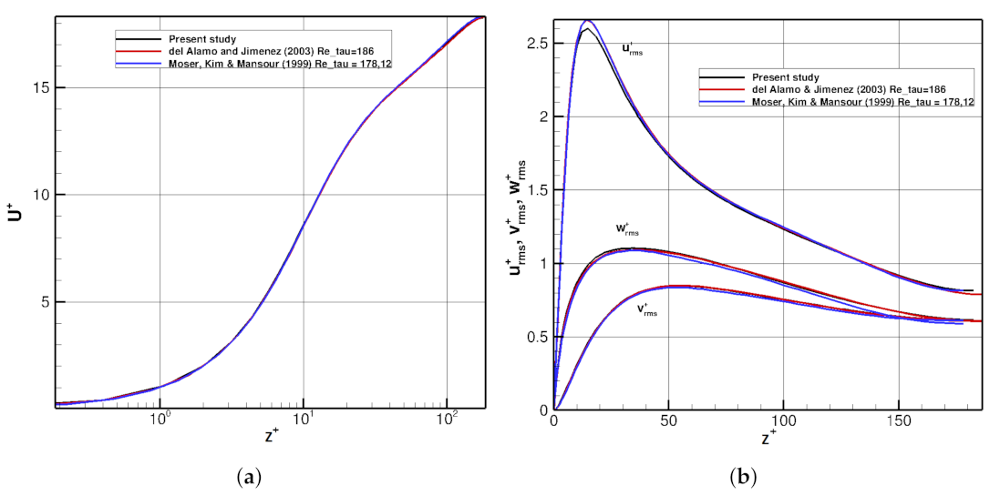
- Moser, R.; Kim, J.; Mansour, N. Direct numerical simulation of turbulent channel flow up to Reτ = 590. Phys. Fluids 1999, 11, 943–945. [Google Scholar] [CrossRef]
- Del Álamo, J.; Jiménez, J. Spectra of the very large anisotropic scales in turbulent channels. Phys. Fluids 2003, 15. [Google Scholar] [CrossRef]
- Sano, M.; Tamai, K. A universal transition to turbulence in channel flow. Nat. Phys. 2016, 12, 249–253. [Google Scholar] [CrossRef] [Green Version]


| 2 | 2820 | 180 | 18 | 918 | 2684 | 977 | |||||
| 10 | 20 | 10 | 8 | 8 | 8 |
| Polynomial order | (Mesh B) | |||
| Planar walls (canonical) | 4.193 × 10 | 4.275 × 10 | 4.397 × 10 | 4.594 × 10 |
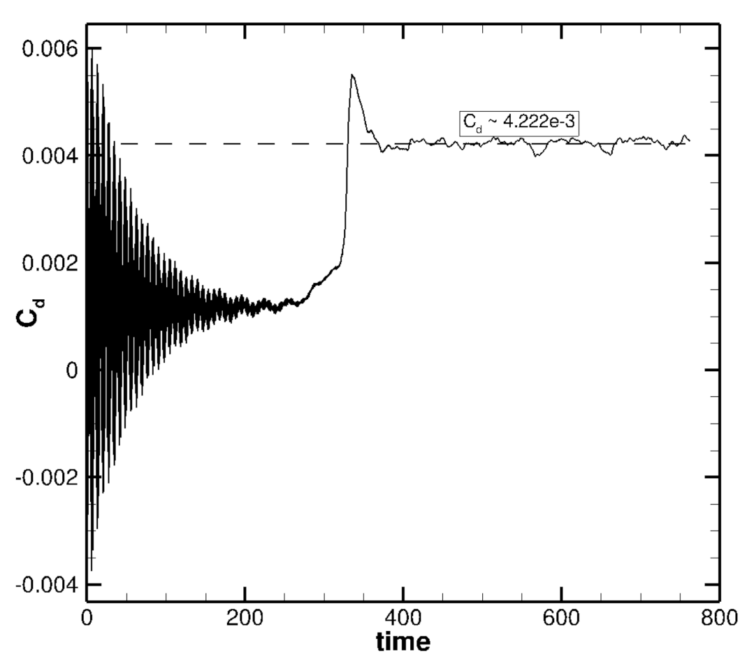
| Wavy walls | 4.145 × 10 | 4.222 × 10 | 4.346 × 10 | 4.549 × 10 |
| Drag Reduction |
Publisher’s Note: MDPI stays neutral with regard to jurisdictional claims in published maps and institutional affiliations. |
© 2021 by the authors. Licensee MDPI, Basel, Switzerland. This article is an open access article distributed under the terms and conditions of the Creative Commons Attribution (CC BY) license (https://creativecommons.org/licenses/by/4.0/).
Share and Cite
Mateo-Gabín, A.; Chávez, M.; Garicano-Mena, J.; Valero, E. Wavy Walls, a Passive Way to Control the Transition to Turbulence. Detailed Simulation and Physical Explanation. Energies 2021, 14, 3937. https://doi.org/10.3390/en14133937
Mateo-Gabín A, Chávez M, Garicano-Mena J, Valero E. Wavy Walls, a Passive Way to Control the Transition to Turbulence. Detailed Simulation and Physical Explanation. Energies. 2021; 14(13):3937. https://doi.org/10.3390/en14133937
Chicago/Turabian StyleMateo-Gabín, Andrés, Miguel Chávez, Jesús Garicano-Mena, and Eusebio Valero. 2021. "Wavy Walls, a Passive Way to Control the Transition to Turbulence. Detailed Simulation and Physical Explanation" Energies 14, no. 13: 3937. https://doi.org/10.3390/en14133937
APA StyleMateo-Gabín, A., Chávez, M., Garicano-Mena, J., & Valero, E. (2021). Wavy Walls, a Passive Way to Control the Transition to Turbulence. Detailed Simulation and Physical Explanation. Energies, 14(13), 3937. https://doi.org/10.3390/en14133937