Applying Wavelet Filters in Wind Forecasting Methods

Abstract

Wind is a physical phenomenon with uncertainties in several temporal scales, in addition, measured wind time series have noise superimposed on them. These time series are the basis for forecasting methods. This paper studied the application of the wavelet transform to three forecasting methods, namely, stochastic, neural network, and fuzzy, and six wavelet families. Wind speed time series were first filtered to eliminate the high-frequency component using wavelet filters and then the different forecasting methods were applied to the filtered time series. All methods showed important improvements when the wavelet filter was applied. It is important to note that the application of the wavelet technique requires a deep study of the time series in order to select the appropriate family and filter level. The best results were obtained with an optimal filtering level and improper selection may significantly affect the accuracy of the results.

1. Introduction

When the penetration of wind power into the network reaches a certain level, system operators have difficulties in balancing generation with demand. To help address this issue, it is necessary to apply forecasting methods to estimate the wind power generated in the next few hours and days.

Several methods have been used to forecast the wind speed: stochastic methods such as the AR [1] and ARIMA [2,3,4] process or heuristic methods such as the Kalman filter [5,6], neural networks [7,8,9], and neuro-fuzzy systems [10,11]. Among all methods, neural networks are the most widely used by researchers.

It is difficult to compare different methods if they do not use the same dataset and the same performance indexes. A typical approach for comparison is to use the persistence model as the reference [12]. Table 1 illustrates the improvement achieved by different forecasting methods compared to the persistence method (although different forecast horizons are used, the list gives an idea of the range of improvement). These improvements are rarely over 25%.

Table 1. Review of forecasting methods.

Authors	Forecast Method	Forecast Horizon	Improvement vs. Persistence Model
[1]	AR	--	--
[2]	ARMA	1–10 h	12–20%
[3]	ARMA	20″–10″	5–12%
[4]	ARMA	6 h	19%
[5]	Kalman filter	1′	4–10%
[6]	Kalman filter	--	--
[7]	ANN	1′–10′	11–8%
[8]	Spatial/ANN	2–2 h	15–25%
[9]	ANN	1′–1 h	--
[10]	Neuro-fuzzy	6–36 h	46%
[11]	Neuro-fuzzy	10′	5%

Wind speed series have considerable uncertainty because of weather fluctuations and the added instrument uncertainty. This uncertainty and noise make it difficult to improve the forecasts. There are several strategies to process the data [13,14,15]. Some authors have used wavelet transforms [16] to process the time series. Most authors [17,18,19,20,21,22,23,24,25,26,27,28,29,30,31] have used wavelets to decompose the time series into sub-series, called approximation and details; applied the forecasting method to each sub-series, and finally, summarized the forecasting results to obtain the final solution. The advantage of this method comes from the sub-series having an improved performance with respect to the original series. A few authors [32,33,34,35,36,37] have used other wavelet filtering techniques to eliminate the high frequency variations and smooth the time series. In all papers, the authors selected the wavelet family and decomposition level without too much justification. For example, the cited authors only used one wavelet family. These works used the wavelet transform as an auxiliary technique and did not study them at sufficient depth.

In this paper, the wavelet transform was analyzed thoroughly. This work demonstrated that the selection of the wavelet family and decomposition level were far more important than they have been given credit for thus far. The improvement obtained was greater than that achieved with most new forecasting methods. The result was applied to the three main forecasting methods currently used, namely statistical, neural network, and fuzzy methods. These were applied to several forecast horizons and sample times. In all cases, the results obtained were improved for each method when the optimal wavelet filter was applied. Finally, the main contribution of the paper is to highlight the importance of data processing and to propose it as an additional phase in the forecasting method, so that both steps are optimized together.

The rest of this paper is structured as follows. Section 2 explains the basic concepts of the wavelet transform. Section 3 presents the different forecasting approaches. Section 4 describes the forecasting approach proposed. In Section 5, the comparison criteria to evaluate the improvement of each method are explained. Section 6 presents the results for the different methods considered. Finally, Section 7 draws the main conclusions of this research.

2. Basic Concepts of the Wavelet Transform

Fourier analysis is commonly used to help analyze different types of signals. With this method, a signal f(t) is expressed as a linear decomposition of real-valued functions of t, as shown in Equation (1),

$$f\left(t\right)={\sum }_k{a}_k{\varphi }_k\left(t\right)$$

(1)

where a_k are the real-valued expansion coefficients and ϕ_k(t) are a set of real-valued functions of t called the expansion set. In Fourier series, these are sin(kω₀t) and cos(kω₀t) with frequencies of kω₀.

2.1. Wavelet Transform

An introduction to the wavelet transform can be found in [16]. In Equation (2), the signal is already decomposed into coefficients a_j,k and functions Ψ_j,k(t), which depend on parameters j and k,

$$f\left(t\right)={\sum }_k{\sum }_j{a}_{j,k}{\Psi }_{j,k}\left(t\right)$$

(2)

where Ψ_j,k are the wavelet expansion functions and a_j,k is the discrete wavelet transform of f(t), or the set of expansion coefficients.

The wavelet expansion functions, or family of wavelets are generated from a mother wavelet Ψ(t) by scaling and translation:

$${\Psi }_{j,k}\left(t\right)=2^{j/2}\Psi \left(2^{j}t-k\right)$$

(3)

where the parameter k translates the function and the parameter j scales it. Figure 1 shows the translating and scaling operations of the function $\Psi \left(2^{j}t-k\right)$.

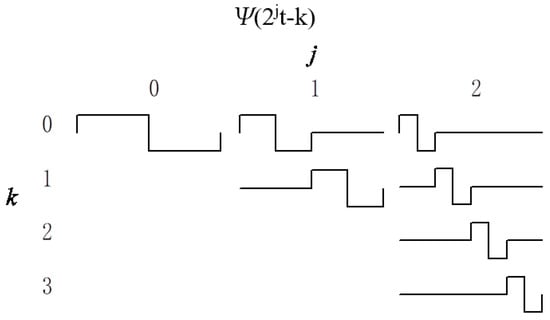
Figure 1. Translating and scaling operations of Ψ(2^jt − k) function.

2.2. Multi-Resolution Formulation of Wavelet Systems

In multi-resolution analysis, the resolution of the approximation of f(t) depends on the choice of j in Equation (2). For a value of j = j0, the equation is:

$$f\left(t\right)={\sum }_k{c}_{j0,k}{\phi }_{j0,k}\left(t\right)$$

(4)

For low values of j, the approximation of f(t) can represent only coarse information. In multi-resolution formulation, φ_j0,k(t) are called scaling functions. If we want to represent detailed information, then high values of j are required.

However, there is another way to describe a signal with better resolution without increasing j. This new approach consists of describing the differences between the approximation and the original signal with a combination of other functions called wavelets Ψ_j,k(t) and the coefficients d_j,k, as shown in Equation (5). The parameters k and j indicate the translation and scaling of the function.

$$\begin{gathered} f\left(t\right)={\sum }_k{c}_{j0,k}{\phi }_{j0,k}\left(t\right)+{\sum }_k{\sum }_{j=jo}^{J-1}{d}_{j,k}{\psi }_{j,k}\left(t\right) \\ ={\sum }_k{c}_{j0}\left(k\right)2^{j0/2}\phi \left(2^{j0}t-k\right)+{\sum }_k{\sum }_{j=jo}^{J-1}{d}_j\left(k\right)2^{j/2}\psi \left(2^{j}t-k\right) \end{gathered}$$

(5)

There are several packets of scaling functions φ(t) and wavelets Ψ(t), as shown in Equation (6) (see Figure 2), which were chosen depending on the signal that has to be approximated.

$$\begin{gathered} \phi \left(t\right)={\sum }_n{h}_0\left(n\right)\sqrt{2}\phi \left(2t-n\right) \\ \psi \left(t\right)={\sum }_n{h}_1\left(n\right)\sqrt{2}\psi \left(2t-n\right) \end{gathered}$$

(6)

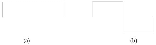
Figure 2. Haar packet. (a) Haar scaling function, φ(t); (b) Haar wavelet function, Ψ(t).

In Equation (6), the coefficients h₀(n) and h₁(n) with n∈Z, are a sequence of real numbers called filter coefficients. The process is similar to digital filters, where h₀(m − 2k) acts as a low-pass filter and h₁(m − 2k) acts as a high-pass filter. Figure 3 shows the decomposition process of c_j in: c_j+1 (low frequency) and d_j+1 (high frequency).

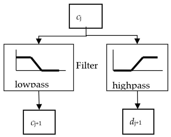
Figure 3. Decomposition process.

The j+1 level scaling coefficients are:

$$\begin{gathered} c_{j+1}\left(k\right)={\sum }_m{h}_0\left(m-2k\right)c_j\left(m\right) \\ {d}_{j+1}\left(k\right)={\sum }_m{h}_1\left(m-2k\right)c_j\left(m\right) \end{gathered}$$

(7)

These expressions represent the approximation and details of the signal for a j + 1 level scaling, and m = 2k + n is a sequence of real numbers.

This process can be repeated iteratively to reduce the high-frequency component as shown in Figure 4.

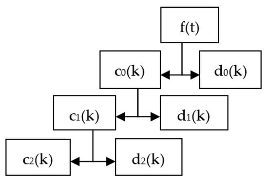
Figure 4. Iterative decomposition.

In Figure 5b, we can see the approximation c₂(k) and the details d₂(k), d₁(k), and d₀(k) of the original signal f(t) are shown in Figure 5a.

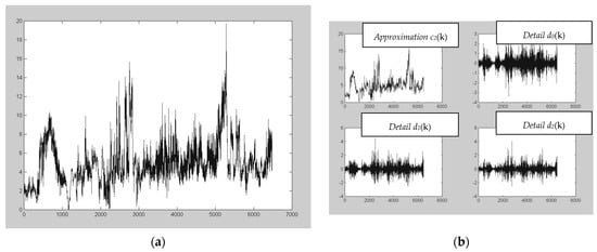
Figure 5. Approximation and details of a signal. (a) Original signal; (b) Approximation c₂(k) and details d₂(k), d₁(k) and d₀(k).

Wind speed time series have a high-frequency component due to wind gusts, measurement errors, and random events as well as a low-frequency component with slower variation. The high-frequency component of the signal introduces a lot of noise into forecasting methods, causing them to perform poorly. If this component is eliminated and the forecasting methods are applied to an approximation with only the low frequency component, improved results can be obtained.

2.3. Wavelet Families

There is a large number of wavelets. The selection of the wavelet function depends on the problem and the properties of the wavelet function [16]. The main properties are its region of support and the number of vanishing moments. The region of support affects its localization capabilities, whereas the vanishing moments limit the ability of the wavelet to represent the information of a signal. In this paper, the wavelet families used were: Haar, Daubechies, Symlet, Coiflet, Biorsplines, and Meyer.

There are some methods to select the optimal wavelet family, but they have been developed for specific applications and it is not certain that they can be applied to forecasting problems:

• In the cross-correlation method [38], the optimum wavelet maximizes the cross-correlation between the signal of interest and the wavelet;
• In the energy method [39], the aim is to maximize the energy of the signal of interest; and
• In the entropy method [40], the best wavelet minimizes the entropy of the signal of interest.

3. Forecasting Models

The wavelet filter was applied to several forecasting methods, namely regression, neural network and fuzzy models.

3.1. Persistence Model

In the persistence model, the variable value in t + Δt is equal to the variable value in t. Due to its simplicity, this model was used as a reference.

$$y_t=y_{t-1}.$$

(8)

3.2. Regressive Model

This model [41] is based on the multiple regressions that study the relations between a dependent variable and a set of independent variables. Among the independent variables, there are exogenous variables such as temperature, and intrinsic variables like the historical values of these variables. When the model only uses the historical values of these variables, it is called the auto-regressive temporal series model. In this work, the model used the historical values:

$$y_t={\sum }_{i=1}^p{\alpha }_i{y}_{t-i}.$$

(9)

where α_i represents the auto-regressive parameters and p is the number of past values.

3.3. Neural Network Model

Neural networks [42] are auto-adaptive dynamic systems that are able to find nonlinear relations between several variables. The model used is a multilayer perceptron that gives good results in forecasting problems:

$$y_t={\sum }_j{w^{\prime }}_{kj}g\left({\sum }_i(w_{ji}{y}_{t-i}-{\mathsf{\theta }}_j)-{{\mathsf{\theta }}^{\prime }}_k\right)$$

(10)

where ${{\mathsf{\theta }}^{\prime }}_j$ and ${{\mathsf{\theta }}^{\prime }}_k$ are the layer thresholds; w_ji and w_kj are the layer weights; i and j are the number of neurons in each layer; and g is the activation function.

3.4. Fuzzy Model

The fuzzy model [43] is based on concepts of fuzzy sets theory, fuzzy rules of type if–then, and approximation reasoning:

$$\{\begin{array}{c}Rj: \mathrm{if}{\cap }_i\left(y_{t-i} \mathrm{is} {\tilde{A}}_i\right) \mathrm{then} u_j={\sum }_i\left(p_i{y}_{t-i}\right)\\ y_t={\sum }_j\left(\frac{{\omega }_j{u}_j}{{\overline{\omega }}_j}\right)\end{array}$$

(11)

where ${\omega }_i$ is the normalized firing strengths; u_i is the functions that depend on the inputs y_t-I; ${\tilde{A}}_i$ is the fuzzy set that represents the input variables; and p_i is the membership grade of each input y_t in ${\tilde{A}}_i$.

4. Forecasting Approach

Wind time series have high variability due to the intrinsic uncertainty of the wind; this variability negatively influences the forecasting result. In this paper, the adopted approach, illustrated in Figure 6, consists of using an optimized filter based on wavelets to de-noise the data that are used to train the chosen forecasting method. The filter is optimized with a genetic algorithm that selects the best wavelet family and the optimal decomposition level.

Figure 6. Flow chart of the forecasting approach.

The algorithm receives as inputs the wind speed data and the prediction method to be used.

In step 1, a random population of individuals is created. Each individual contains the information of the parameters of the prediction method, the wavelet family, and the level of decomposition.

In step 2, each individual in the population is evaluated. The evaluation has three phases.

The first phase consists of applying the wavelet filter to the input data with the wavelet family and the level indicated by each individual. The data are divided into training and test sets. The original time series is filtered with the wavelet transform and is decomposed into an approximation component and several details of the signal. The approximation component has improved behavior in comparison to the original series in the forecasting process. Therefore, only the approximation component is used in the next phase and the details are discarded. In this phase, there are two important decisions to analyze: the best wavelet family to use and the optimal filter level. These questions have not been answered in the technical literature.

The second phase consists of training the prediction method with the parameters indicated by each individual and the training dataset. A forecasting method is applied only to the approximation component. In this paper, three methods were used to forecast the time series: autoregressive, neural networks, and fuzzy models.

The third phase consists of evaluating the prediction method, already trained, with the test dataset.

In step 3, the best individuals are selected based on the error obtained in the evaluation with the test data.

In step 4, the crossover and mutation operators of the genetic algorithm are applied that give rise to a new population.

Steps 2 through 4 are repeated until the termination criterion is reached, which is the number of generations or iterations of the genetic algorithm.

5. Forecasting Errors

We compared these forecasting methods with the simpler persistence model used as the reference. The measure of the error of each method was calculated by the root mean square error (RMSE),

$$\mathrm{RMSE}=\sqrt{\frac{{\sum }_{t=1}^n{\left({\mathrm{Xpred}}_t-{\mathrm{Xreal}}_t\right)}^2}{n}}$$

(12)

where Xpred_t is the predicted value in t; Xreal_t is the real value at t; and n is the number of samples.

The improvement of each method in comparison to the persistence model was calculated with the following equation:

$$\mathrm{Improvement} \mathrm{vs}. \mathrm{persistence} (\%)=\frac{\mathrm{RMSE}\left(\mathrm{persistence}\right)-\mathrm{RMSE}\left(\mathrm{method}\right)}{\mathrm{RMSE}\left(\mathrm{persistence}\right)}$$

(13)

6. Results of Validation Cases

6.1. Data Description

The wavelet filter was applied to several forecasting methods: regression, neural network, and fuzzy models. Five wind speed series were used in this work: two series with a high sampling frequency (1″ and 1′, respectively) and three with a sampling frequency of 10′. Table 2 shows the main statistic characteristics of these time series and Figure A1, Figure A2, Figure A3, Figure A4 and Figure A5 in the Appendix A represent their temporal variation.

Table 2. Time series description.

Time Series	Mean	Standard Deviation	Maximum	Skewness	Kurtosis	Size	Sampling Frequency
I	5.281	1.862	12.597	0.643	3.139	1 month	1″
II	4.951	2.313	19.726	1.212	5.467	1 month	1′
III	8.258	4.709	34.690	1.115	4.815	2 years	10′
IV	8.308	9.883	30.000	1.124	2.873	2 years	10′
V	6.848	3.548	27.020	0.684	3.406	2 years	10′

Several cases were built from these data to observe the performance of the forecasting models when the sampling step (Δt) and the forecasting horizon (FH) changed. An identifier (ID) was assigned to each case in Table 3.

Table 3. Case description.

T.S.-I			T.S.-II			T.S.-III			T.S.-IV			T.S.-V
ID	FH.	Δt	ID	FH.	Δt	ID	FH.	Δt	ID	FH.	Δt	ID	FH.	Δt
1	1′	5″	11	2 h	5′	21	10′	10′	26	10′	10′	31	10′	10′
2	5′	5″	12	2 h	10′	22	1 h	1 h	27	1 h	1 h	32	1 h	1 h
3	5′	10″	13	6 h	10′	23	6 h	6 h	28	6 h	6 h	33	6 h	6 h
4	5′	20″	14	6 h	30′	24	12 h	12 h	29	12 h	12 h	34	12 h	12 h
5	10′	10″	15	12 h	10′	25	24 h	24 h	30	24 h	24 h	35	24 h	24 h
6	10′	20″	16	12 h	30′
7	10′	30″	17	12 h	1 h
8	20′	30″	18	24 h	30′
9	20′	1′	19	24 h	1 h
10	1 h	1′	20	24 h	2 h

6.2. Results

Every time series was divided into two sets of the same length: a training set and a test set. The forecasting models were built with the training set and the results presented here were obtained by applying these models to the test set. Moreover, eight inputs were used in all methods.

First, a detailed analysis of wavelet filtering is presented, aiming to answer whether they are helpful with different prediction methods and whether they depend on factors such as the level of filtering, the prediction horizon, and the sampling frequency. Afterward, we analyze whether it is possible to select the wavelet family by any of the methods described in the literature regardless of the prediction method used. Finally, its application is presented in a specific case.

6.2.1. Influence of Wavelet Filters in Several Forecasting Methods

The best obtained results of applying the wavelet filters on time series are presented in Figure 7 and Figure 8. It is shown that regardless of the model, the forecasting horizon, or time step, the performance was much better with the wavelet filter than without it when the optimal wavelet family and level were chosen.

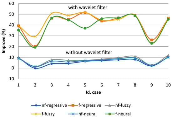
Figure 7. Time series I: Improve versus persistence.

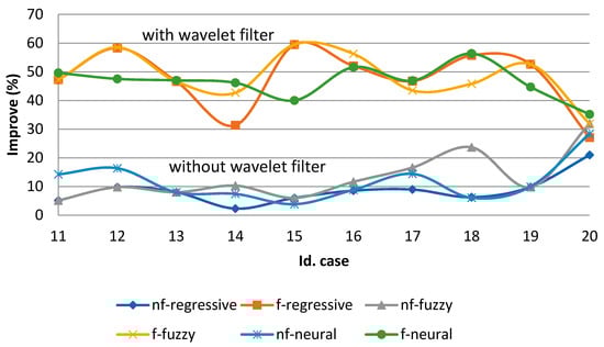
Figure 8. Time series II: Improve versus persistence.

Detailed results are provided in Table A1, Table A2, Table A3, Table A4, Table A5 and Table A6 in the Appendix A. It is important to note that the optimal wavelet family and level was different in each case. That is, there was a lot of variability in this point. This fact is contrary to the widespread action among researchers who choose these parameters depending on the application.

6.2.2. Influence of Decomposition Level

However, there was a great similarity in the performance of the different wavelet families in each case. Each family reached different levels of improvement, but all families achieved their maximum improvement percentage at a similar level. Figure 9 shows the improvement/level rate for a particular case, with different forecasting methods. Figure 10 shows the improvement/level rate of the same case and method for different wavelet families (see Table A10, Table A11, Table A12 and Table A13 for details).

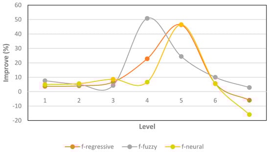
Figure 9. Case 3: Improve versus level for the best family.

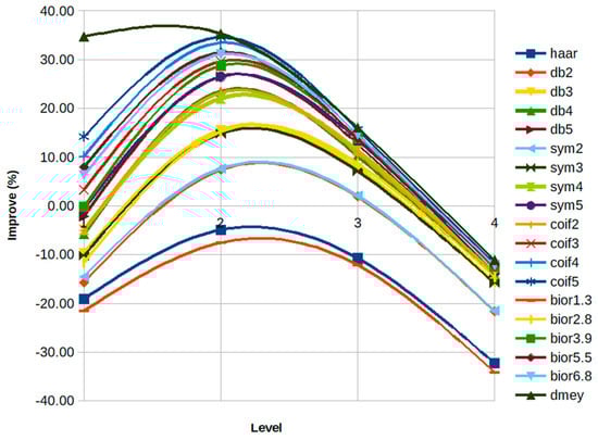
Figure 10. Case 31: Improvement percentage versus level for all families with neural model.

The last results explain why researchers can obtain favorable solutions by applying wavelets, even when they do not select the wavelet family and level accurately.

6.2.3. Influence of the Forecasting Horizon

Comparisons made up to now were in percent, because it permitted us to adequately show the difference between whether the wavelet filters were applied or not. However, it is necessary to remember that the error (RMSE) increased with the forecasting horizon, as can be seen in Figure 11, Figure 12 and Figure 13, although less when the wavelet filters were applied.

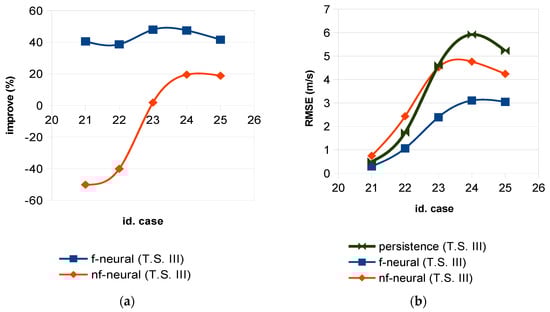
Figure 11. Time series III: (a) Improvement percentage versus persistence; (b) RMSE.

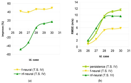
Figure 12. Time series IV: (a) Improvement percentage versus persistence; (b) RMSE.

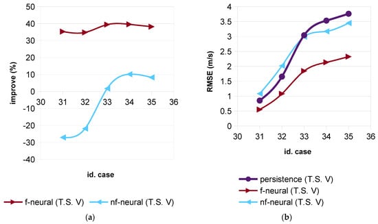
Figure 13. Time series V: (a) Improvement percentage versus persistence; (b) RMSE.

6.2.4. Influence of Different Sampling Frequencies

In Figure 14, it can be seen that with low filtering levels, an important improvement was obtained, but with high filtering levels, information was lost and the improvement decreased or even worsened substantially at high sampling frequencies.

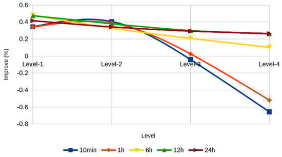
Figure 14. Different sampling frequencies in series III using the dmey wavelet filter.

6.2.5. Selection of Optimal Wavelet Family

In Table 4, the wavelet families found by the cross-correlation, energy, and entropy methods are shown in the columns “cross-corr”, “energy”, and “entropy”, respectively. The column “optimum” shows the wavelet family that gave the best results in our tests.

Table 4. Selection of wavelet family.

Case	Optimum	Cross-Corr	Energy	Entropy	Case	Optimum	Cross-Corr	Energy	Entropy
1	dmey	Bior5.5	dmey	sym5	21	dmey	Haar-bior1.3	Bior6.8	Bior1.3
2	db2	Bior5.5	dmey	sym5	22	dmey	Haar-bior1.3	Bior6.8	Bior1.3
3	Bior2.8	Bior5.5	dmey	dmey	23	Bior6.8	Bior5.5	dmey	Bior1.3
4	db3	Bior5.5	dmey	db2	24	Bior6.8	Bior5.5	dmey	Bior1.3
5	dmey	Bior5.5	dmey	dmey	25	dmey	Bior5.5	dmey	Bior1.3
6	db5	Bior5.5	dmey	db2	26	dmey	Haar-bior1.3	Bior6.8	Bior1.3
7	Bior5.5	Bior5.5	dmey	Bior1.3	27	dmey	Haar-bior1.3	dmey	Bior1.3
8	db2	Bior5.5	dmey	Bior1.3	28	Bior6.8	Bior5.5	dmey	Bior1.3
9	db2	Bior5.5	dmey	db5	29	coif3	Bior5.5	dmey	Bior1.3
10	Bior3.9	Bior5.5	dmey	db5	30	Bior5.5	Bior5.5	dmey	db2-sym2
11	sym4	Bior5.5	dmey	Bior1.3	31	Bior5.5	Bior5.5	Bior5.5	Bior1.3
12	coif3	Bior5.5	dmey	sym4	32	dmey	Bior5.5	dmey	Bior1.3
13	dmey	Bior5.5	dmey	sym4	33	dmey	Bior5.5	dmey	dmey
14	db4	Bior5.5	dmey	Bior1.3	34	dmey	Bior5.5	dmey	Bior2.8
15	dmey	Bior5.5	dmey	sym4	35	dmey	Bior5.5	dmey	db2-sym2
16	sym5	Bior5.5	dmey	Bior1.3
17	coif4	Bior5.5	Bior6.8	sym3
18	dmey	Bior5.5	dmey	Bior1.3
19	Bior3.9	Bior5.5	Bior6.8	sym3
20	db4	Bior5.5	Bior6.8	coif5

These methods were applied to the time series with poor results. The cross-correlation method obtained the correct result in cases 7, 30, and 31; the energy method in cases 1, 5, 13, 15, 18, 25, 27, 32, 33, 34 and 3; and the entropy method in cases 5 and 33.

6.2.6. Applying the Forecasting Approach

The importance of using filtered data is illustrated in the following example. Figure 15 shows the first 300 data points (to appreciate it in detail) of the original data series of case 22, the data series filtered with the wavelet family “dmey” and a filter level 2, and the difference between the two series. Figure 16 shows the results of the forecast made with the neural network trained with the filtered data training set, and Figure 17 shows the results of the forecast made with the neural network trained with the unfiltered data training set. The results using correctly filtered data were considerably better than those with the unfiltered data.

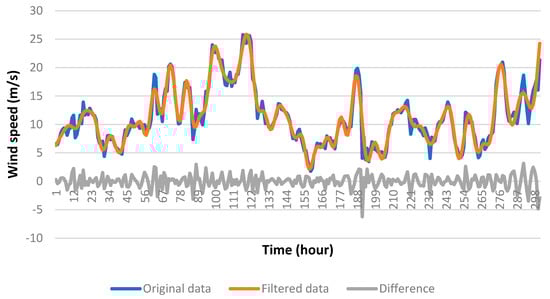
Figure 15. Wavelet filtered process in case 22.

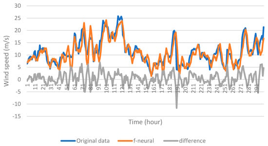
Figure 16. Forecasting result for case 22 with the neural network method trained with filtered data.

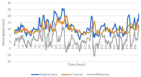
Figure 17. Forecasting result for case 22 with the neural network method trained with unfiltered data.

7. Conclusions

In this paper, the forecasting models were applied to the approximation component of the wavelet decomposition and the details components were discarded, as opposed to most authors who use both components in their forecasting models.

A deep analysis of the wavelet filter in results was made, and the conclusions will enable improvements in all forecasting models.

The wavelet filter method was applied to different forecasting models: regression, neural network, and fuzzy models. In all models, this technique (wavelet filter + forecasting model) improved the obtained results compared to the case when only the forecasting model was used. The improvement of these methods versus the persistence method was between 2% and 30%, but with the wavelet filter method, it was between 20% and 50%.

The study was extended to several wavelet families. In all cases, there were improvements, but it was not easy to select the best family. The selection methods did not work for the proposed method.

The filtering level was more important to obtain good results than the wavelet family in most of cases. This optimum level was between 2 and 5 in all wavelet families.

As a final conclusion, it seems necessary to use an optimization algorithm to select the wavelet family and level.

It has become clear that it is not easy to determine the parameters of the data processing methods and that they significantly influence the results obtained. Hence, future research is the joint optimization of the data processing and the forecasting method.

References

- Brown, B.G.; Katz, R.W.; Murphy, A.H. Time Series Models to Simulate and Forecast Wind Speed and Wind Power. J. Clim. Appl. Meteorol. 1984, 23, 1184–1195. [Google Scholar] [CrossRef]
- Torres, J.; García, A.; de Blas, M.; de Francisco, A. Forecast of hourly average wind speed with ARMA models in Navarre (Spain). Sol. Energy 2005, 79, 65–77. [Google Scholar] [CrossRef]
- Bossanyi, E.A. Stochastic Wind Prediction for Wind Turbine System Control. In Proceedings of the 7th BWEA Wind Energy Conference, Oxford, UK, 27–29 March 1985. [Google Scholar]
- Hill, D.C.; McMillan, D.; Bell, K.R.W.; Infield, D. Application of Auto-Regressive models to U.K. wind speed data for power system impact studies. IEEE Trans. Sustain. Energy 2012, 3, 134–141. [Google Scholar] [CrossRef]
- Bossanyi, E.A. Short-Term Wind Prediction using Kalman Filters. Wind Eng. 1985, 9, 1–8. [Google Scholar]
- Djurovic, M.; Stankovic, L. Predicition of Wind Characteristics in Short-Term Periods. In Energy and the Environment into the 1990s, Proceedings of the 1st World Renewable Energy Congress, Reading, UK, 23–28 September 1990; Pergamon Press: Oxford, UK; New York, NY, USA, 1990. [Google Scholar]
- Beyer, H.G. Short-Term Prediction of Wind-Speed and Power Output of a Wind Turbine with Neural Networks. In Proceedings of the 5th European Community Wind Energy Conference, ECWEC’94, Thessaloniki, Greece, 10–14 October 1994. [Google Scholar]
- Alexiadis, M.C.; Dokopoulos, P.S.; Sahsamanoglou, H.S. Wind speed and power forecasting based on spatial correlation models. IEEE Trans. Energy Convers. 1999, 14, 836–842. [Google Scholar] [CrossRef]
- Flores, P.; Tapia, A.; Tapia, G. Application of a control algorithm for wind speed prediction and active power generation. Renew. Energy 2005, 30, 523–536. [Google Scholar] [CrossRef]
- Sideratos, G.; Hatziargyriou, N.D. An Advanced Statistical Method for Wind Power Forecasting. IEEE Trans. Power Syst. 2007, 22, 258–265. [Google Scholar] [CrossRef]
- Potter, C.W.; Negnevitsky, W. Very short-term wind forecasting for Tasmanian power generation. IEEE Trans. Power Syst. 2006, 21, 965–972. [Google Scholar] [CrossRef]
- Sfetsos, A. A comparison of various forecasting techniques applied to mean hourly wind speed time series. Renew. Energy 2000, 21, 23–35. [Google Scholar] [CrossRef]
- Liu, H.; Chen, C. Data processing strategies in wind energy forecasting models and applications: A comprehensive review. Appl. Energy 2019, 249, 392–408. [Google Scholar] [CrossRef]
- Qian, Z.; Pei, Y.; Zareipour, H.; Chen, N. A review and discussion of decomposition based hybrid models for wind energy forecasting applications. Appl. Energy 2019, 235, 939–953. [Google Scholar] [CrossRef]
- Huang, N.T.; Xing, E.K.; Cai, G.W.; Yu, Z.Y.; Qi, B.; Lin, L. Short-term wind speed forecasting based on low redundancy feature selection. Energies 2018, 11, 1638. [Google Scholar] [CrossRef]
- Sidney Burrus, C.; Gopinath, R.A.; Guo, H. Introduction to Wavelets and Wavelet Transforms; Prentice Hall: Upper Saddle River, NJ, USA, 1998. [Google Scholar]
- Catalão, J.P.S.; Pousinho, H.M.I.; Mendes, V.M.F. Hybrid Wavelet-PSO-ANFIS Approach for Short-Term Wind Power Forecasting in Portugal. IEEE Trans. Sustain. Energy 2010, 2, 50–59. [Google Scholar] [CrossRef]
- Liu, H.; Tian, H.-Q.; Pan, D.-F.; Li, Y.-F. Forecasting models for wind speed using wavelet, wavelet packet, time series and Artificial Neural Networks. Appl. Energy 2013, 107, 191–208. [Google Scholar] [CrossRef]
- Cao, L.; Li, R. Short-term wind speed forecasting model for wind farm based on wavelet decomposition. In Proceedings of the Third International Conference on Electric Utility Deregulation and Restructuring and Power Technologies, DRPT 2008, Nanjing, China, 6–9 April 2008; pp. 2525–2529. [Google Scholar]
- Yao, C.; Yu, Y. A Hybrid Model to Forecast Wind Speed Based on Wavelet and Neural Network. In Proceedings of the International Conference on Control, Automation and Systems Engineering (CASE), Singapore, 30–31 July 2011; 2011; pp. 1–4. [Google Scholar]
- Khan, A.A.; Shahidehpour, M. One day ahead wind speed forecasting using wavelets. In Proceedings of the Power Systems Conference and Exposition PSCE ‘09, Seattle, WA, USA, 15–18 March 2009; pp. 1–5. [Google Scholar]
- Mishra, S.; Sharma, A.; Panda, G. Wind power forecasting model using complex wavelet theory. In Proceedings of the International Conference on Energy, Automation, and Signal (ICEAS), Bhubaneswar, India, 28–30 December 2011; pp. 1–4. [Google Scholar]
- Tong, J.-L.; Zhao, Z.-B.; Zhang, W.-Y. A New Strategy for Wind Speed Forecasting Based on Autoregression and Wavelet Transform. In Proceedings of the 2nd International Conference on Remote Sensing, Environment and Transportation Engineering (RSETE), Nanjing, China, 1–3 June 2012; pp. 1–4. [Google Scholar]
- Li, Y.F.; Wu, H.P.; Liu, H. Multi-step wind speed forecasting using EWT decomposition, LSTM principal computing, RELM sub-ordinate computing and IEWT reconstruction. Energy Convers. Manag. 2018, 167, 203–219. [Google Scholar] [CrossRef]
- Liu, H.; Duan, Z.; Han, F.-Z.; Li, Y.-F. Big multi-step wind speed forecasting model based on secondary decomposition, ensemble method and error correction algorithm. Energy Convers. Manag. 2018, 156, 525–541. [Google Scholar] [CrossRef]
- Liu, H.; Mi, X.; Li, Y. Comparison of two new intelligent wind speed forecasting approaches based on Wavelet Packet Decomposition, Complete Ensemble Empirical Mode Decomposition with Adaptive Noise and Artificial Neural Networks. Energy Convers. Manag. 2018, 155, 188–200. [Google Scholar] [CrossRef]
- Chitsaz, H.; Amjady, N.; Zareipour, H. Wind power forecast using wavelet neural network trained by improved Clonal selection algorithm. Energy Convers. Manag. 2015, 89, 588–598. [Google Scholar] [CrossRef]
- Esfetang, N.N.; Kazemzadeh, R. A novel hybrid technique for prediction of electric power generation in wind farms based on WIPSO, neural network and wavelet transform. Energy 2018, 149, 662–674. [Google Scholar] [CrossRef]
- Zhang, Y.; Zhang, C.; Gao, S.; Wang, P.; Xie, F.; Cheng, P.; Lei, S. Wind Speed Prediction Using Wavelet Decomposition Based on Lorenz Disturbance Model. IETE J. Res. 2018, 66, 635–642. [Google Scholar] [CrossRef]
- Hu, J.; Wang, J.; Ma, K. A hybrid technique for short-term wind speed prediction. Energy 2015, 81, 563–574. [Google Scholar] [CrossRef]
- Wang, J.-Z.; Wang, Y.; Jiang, P. The study and application of a novel hybrid forecasting model—A case study of wind speed forecasting in China. Appl. Energy 2015, 143, 472–488. [Google Scholar] [CrossRef]
- Zhang, W.; Wang, J.; Wang, J.; Zhao, Z.; Tian, M. Short-term wind speed forecasting based on a hybrid model. Appl. Soft Comput. 2013, 13, 3225–3233. [Google Scholar] [CrossRef]
- Liu, D.; Niu, D.; Wang, H.; Fan, L. Short-term wind speed forecasting using wavelet transform and support vector machines optimized by genetic algorithm. Renew. Energy 2014, 62, 592–597. [Google Scholar] [CrossRef]
- Zhang, Y.; Li, R.; Zhang, J. Optimization scheme of wind energy prediction based on artificial intelligence. Environ. Sci. Pollut. Res. 2021, 1–16. [Google Scholar] [CrossRef]
- Yu, C.; Li, Y.; Zhang, M. An improved Wavelet Transform using Singular Spectrum Analysis for wind speed forecasting based on Elman Neural Network. Energy Convers. Manag. 2017, 148, 895–904. [Google Scholar] [CrossRef]
- Mi, X.-W.; Liu, H.; Li, Y.-F. Wind speed forecasting method using wavelet, extreme learning machine and outlier correction algorithm. Energy Convers. Manag. 2017, 151, 709–722. [Google Scholar] [CrossRef]
- Cheng, L.; Zang, H.; Ding, T.; Sun, R.; Wang, M.; Wei, Z.; Sun, G. Ensemble Recurrent Neural Network Based Probabilistic Wind Speed Forecasting Approach. Energies 2018, 11, 1958. [Google Scholar] [CrossRef]
- Ma, X.; Zhou, C.; Kemp, I.J. Automated wavelet selection and thresholding for PD detection. IEEE Electr. Insul. Mag. 2002, 18, 37–45. [Google Scholar] [CrossRef]
- Donoho, D. De-noising by soft-thresholding. IEEE Trans. Inf. Theory 1995, 41, 613–627. [Google Scholar] [CrossRef]
- Coifman, R.; Wickerhauser, M. Entropy-based algorithms for best basis selection. IEEE Trans. Inf. Theory 1992, 38, 713–718. [Google Scholar] [CrossRef]
- Draper, N.R.; Smith, H. Applied Regression Analysis; John Wiley: Hoboken, NJ, USA, 1998. [Google Scholar]
- Tsoukalas, L.H.; Uhrigh, R.E. Fuzzy and Neural Approaches in Engineering; Wiley-Blackwell: Hoboken, NJ, USA, 1997. [Google Scholar]
- Jang, J.S.R. ANFIS: Adaptive-Network-Based Fuzzy Inference System. IEEE Trans. Syst. Man Cybern. 1993, 23, 665–685. [Google Scholar] [CrossRef]
Publisher’s Note: MDPI stays neutral with regard to jurisdictional claims in published maps and institutional affiliations. |
© 2021 by the authors. Licensee MDPI, Basel, Switzerland. This article is an open access article distributed under the terms and conditions of the Creative Commons Attribution (CC BY) license (https://creativecommons.org/licenses/by/4.0/).