Short Term Active Power Load Prediction on A 33/11 kV Substation Using Regression Models

Abstract

Electric power load forecasting is an essential task in the power system restructured environment for successful trading of power in energy exchange and economic operation. In this paper, various regression models have been used to predict the active power load. Model optimization with dimensionality reduction has been done by observing correlation among original input features. Load data has been collected from a 33/11 kV substation near Kakathiya University in Warangal. The regression models with available load data have been trained and tested using Microsoft Azure services. Based on the results analysis it has been observed that the proposed regression models predict the demand on substation with better accuracy.

1. Introduction

Electric power industries are seeking electric power prediction tools to forecast the load so that balance between load and generation can be maintained properly. Prediction of active power load is required for arranging regular interval activities and power firms are increasing their infrastructure [1]. Accurate load forecasting systems provide a better understanding of the dynamics of existing power systems [2]. Electric load forecasting was classified into three categories as presented in Table 1 based on time horizon [3].

Table 1. Active power load prediction classification.

Load Prediction Type	Time	Usage
Short term	Few hours to days	Electric power generation and transmission scheduling
Medium term	Few weeks to months	Fuel purchase scheduling
Long term	1–10 years	Establishment of power sector entities

Short-term active power load prediction is vital to effective power system service, such as dispatching power into the network to prevent regular power outages. Short term active power estimation is a critical prerequisite for optimal dispatch of generators in power plants [4]. Customers would be able to select a more cost-effective energy usage scheme if the short-term load forecasting methodology was more accurate. It helps the power system to reduce cost of power production and to utilize resources optimally [5].

Artificial Intelligence (AI) is an integral part of many fields, some of the main subparts of AI are machine learning and swarm intelligence. Machine learning has become an integral part in many fields like civil engineering applications [6,7], image processing [8] and time series data prediction [9]. Swarm intelligence was developed by taking inspiration from the swarming behavior of various natural systems and this is used to solve various optimization problems [10,11].

Estimation methods to predict the active power load was classified into two classes as shown in Figure 1. Prediction tools were used to estimate solar irradiation, temperature and wind speed. ARIMA time series forecast model was developed in [12] to predict the temperature in Pakistan and it also develops a linear trend model to estimate electric power consumption. Digital Elevation Models were developed in [13] to predict the solar irradiation.

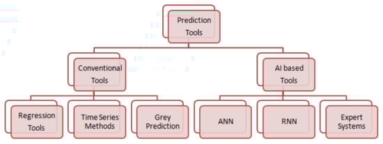
Figure 1. Prediction tools.

Forecasting techniques can help power system operators exchange active power for the highest possible benefit by calculating active power load and energy price. Electric energy price was predicted using artificial neural networks in [14] by considering day category, hour marker, holiday index, electric load, nonconventional energy generation and natural gas price as input features.

A new model was developed in [15] to predict the active power load. Active power load was estimated in [16] by considering day category, hour marker, holiday index, electric load, renewable energy generation using artificial neural networks and MLR model. Active power load was predicted in [17] based on load data of last four hours. Active power load was estimated in [18,19,20] based on load data for the last four hours and load data at the same hour for the last two days.

An ANN model was developed in [21] to forecast the half-hourly electric load demand in Tunisia. Authors have used a Levenberg–Marquardt learning algorithm to train the ANN model. Prediction of electricity demand and price one day ahead using functional models was discussed in [22]. Estimation of electric power consumption in Shanghai using grey forecasting model was discussed in [23]. All of these methods make useful advancements to load estimation, but these overlook useful elements such as dimensionality reduction, which improves model accuracy per number of model parameters.

In this paper, stochastic gradient descent optimizer [24] was used to update the parameters in the regression models. The methods described are analyzed by comparing them to previously developed models [17,18].

The main contributions of this paper are as follows:

• SLR and PR models were used to predict the active power load.
• A new approach, i.e., predict the active power load based on load at last three hours and load at one day before was used with various regression models and dimensionality reduction technique was used to reduce the complexity of the model so that overfitting problem was removed.
• Data analytic tools were used to process the data before feeding it to the model

2. Methodology

Active power load on a 33/11 kV substation has been predicted using regression models like SLR, MLR and PR. In all regression models, stochastic gradient optimizer has been used to update the parameters so that error, i.e., the difference between actual and predicted load is minimum.

2.1. Simple Linear Regression Model (SLR)

In SLR, output variable ($Y_a$) is related linearly with input variable ($X_a$). For a given input $X_a$, predicted output Y will be calculated using Equation (1). Gradient descent optimization method has been used to find the values of m and c for the given inputs ($X_a$) and corresponding outputs ($Y_a$), such that the total distance between all the output data points and line represented by Equation (1) is minimum, as shown in Figure 2. The main objective of gradient descent optimization method is minimization of half mean distance from all actual data points from line as shown in Equation (2). This half mean distance is also called error which represents the difference between actual output $Y_a$ and predicted output (Y). As error which is going to minimize is a convex function, the gradient descent optimizer will perform well to reach global minimum point.

$$Y=m{X}_a+c$$

(1)

$$MinE=\frac{d_1+d_2+d_3+d_4+...+d_s}{2n_s}=\sum _{a=1}^{n_s}\frac{d_a}{2n_s}=\sum _{a=1}^s\frac{\sqrt{{(Y_a-Y)}^2}}{2n_s}$$

(2)

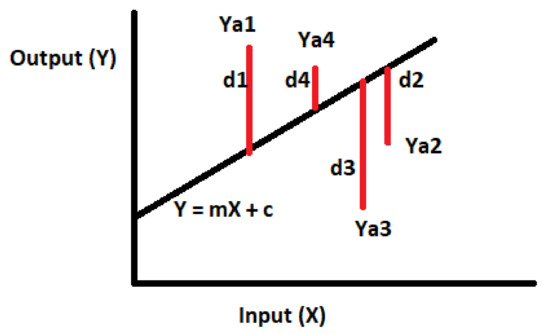
Figure 2. Distance between actual output (Ya) and predicted output (Y).

Gradient descent optimizer will update the solution such that it will reach the point where gradient is zero by choosing step size opposite to the gradient. In linear regression problem m and c are variables and step size for m, i.e., $\delta m$ and step size for c, i.e., $\delta c$ has been computed using Equations (3) and (4) respectively. Variables m and c will be updated using Equations (5) and (6), respectively, such that gradient will reach towards zero.

$$\delta m=-\eta \frac{\partial E}{\partial m}=\sum _{a=1}^{n_s}\eta (Y_a-m{X}_a-C)X_a$$

(3)

$$\delta c=-\eta \frac{\partial E}{\partial c}=\sum _{a=1}^{n_s}\eta (Y_a-m{X}_a-C)$$

(4)

$$m=m+\delta m$$

(5)

$$c=c+\delta c$$

(6)

SLR has been used to predict the active power load (L(D, t)) on a substation at particular hour (t) of the day (D) based on active power load (L(D−1, t)) at same time (t) but in previous day (D−1). In this scenario L(D−1, t) data points represent input ($X_a$), whereas L(D, t) data points represents output ($Y_a$). The procedure for load prediction using SLR is presented in Figure 3.

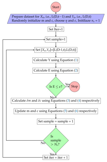
Figure 3. Simple Linear Regression model training algorithm.

2.2. Multiple Linear Regression Model (MLR)

In MLR, output variable ($Y_a$) is related linearly with multiple input variables like ($X_1^a$, $X_2^a$, ⋯, $X_n^a$). For a given input variables ($X_1^a$, $X_2^a$, ⋯, $X_n^a$), output Y will be predicted using Equation (7). Gradient descent optimization method has been used to find the values of ($m_1$, $m_2$, ⋯, $m_n$) and c for the given inputs ($X_a$) and corresponding outputs ($Y_a$), such that the half mean distance between all the output data points and line represented by Equation (7) is minimum as shown in Figure 4.

$$Y=m_1{X}_1^a+m_2{X}_2^a+...+m_n{X}_n^a+c$$

(7)

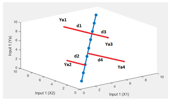
Figure 4. Distance between actual output (Ya) and predicted output (Y) for MLR.

In MLR the variables step size like $\delta m_i$ $ϵ$ ($\delta m_1$, $\delta m_2$, ⋯, $\delta m_n$) and $\delta c$ have been computed using Equations (8) and (9) respectively. Variables $\delta m_i$ $ϵ$ ($m_1$, $m_2$, ⋯, $m_n$) and c will be updated using Equations (6) and (10) respectively such that gradient will reach toward zero.

$$\delta m_i=-\eta \frac{\partial E}{\partial m_i}=\sum _{a=1}^{n_s}\eta (Y_a-\sum _{i=1}^n{m}_i{X}_i^a-C)X_i^a$$

(8)

$$\delta c=-\eta \frac{\partial E}{\partial c}=\sum _{a=1}^{n_s}\eta (Y_a-\sum _{i=1}^n{m}_i{X}_i^a-C)$$

(9)

$$m_i=m_i+\delta m_i$$

(10)

MLR has been used to predict the active power load (L(D,t)) on a substation at particular hour (t) of the day (D) based on last three hours load data from time of prediction, i.e., L(D, t−1), L(D, t−2), L(D, t−3) and active power load (L(D−1, t)) at same time (t) but in previous day (D−1). In this scenario L(D, t−1), L(D, t−2), L(D, t−3) and L(D−1, t) data points represent input ($X_a$), whereas L(D,t) data points represents output ($Y_a$). The procedure for load prediction using MLR is presented in Figure 5.

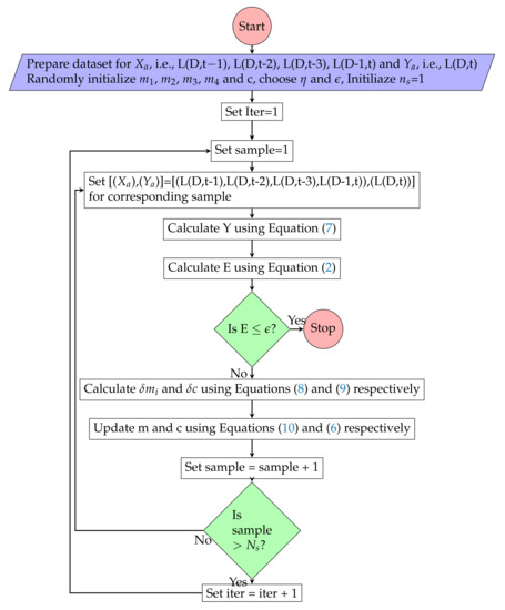
Figure 5. Multiple linear regression model training algorithm.

2.3. Polynomial Regression Model (PR)

In PR, output variable ($Y_a$) is related nonlinearly with input variable ($X_a$). For a given input $X_a$, output Y will be predicted using Equation (11). Gradient descent optimization method has been used to find the values of ($m_1$, $m_2$, ⋯, $m_p$) and c for the given input ($X_a$) and corresponding outputs ($Y_a$), such that the total distance between all the output data points and nonlinear curve represented by Equation (11) is minimum as shown in Figure 6. The main objective of gradient descent optimization method is minimization of half mean distance from all actual data points from nonlinear curve as shown in Equation (2).

$$Y=m_p{X}_a^p+m_{p-1}{X}_a^{p-1}+...+m_1{X}_a+c$$

(11)

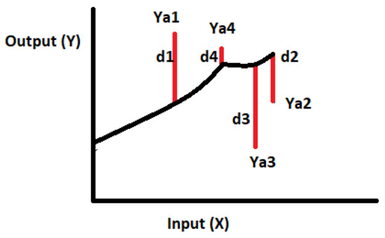
Figure 6. Distance between actual output (Ya) and predicted output (Y).

Gradient descent optimizer will update the solution such that it will reach the point where gradient is zero by choosing step size opposite to the gradient. In PR problem ($m_1$, $m_2$, ⋯, $m_p$) and c are variables and step size for $m_i$, i.e., $\delta m_i$ and step size for c, i.e., $\delta c$ have been computed using Equations (12) and (13) respectively. Variables $\delta m_i$ and c will be updated using Equations (6) and (10), respectively, such that gradient will reach toward zero.

$$\delta m_i=-\eta \frac{\partial E}{\partial m_i}=\sum _{a=1}^{n_s}\eta (Y_a-\sum _{i=1}^p{m}_i{X}_a^i-c)X_a^i$$

(12)

$$\delta c=-\eta \frac{\partial E}{\partial c}=\sum _{a=1}^{n_s}\eta (Y_a-\sum _{i=1}^p{m}_i{X}_a^i-c)$$

(13)

PR model has been used to predict the active power load (L(D,t)) on a substation at particular hour (t) of the day (D) based on active power load (L(D−1,t)) at same time (t) but in previous day (D−1). In this scenario L(D,t) data points represents output ($Y_a$), whereas L(D−1,t) data points represent input ($X_a$). The procedure for load prediction using PR is presented in Figure 7.

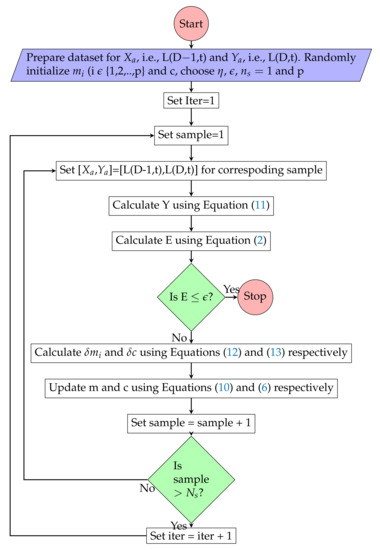
Figure 7. Polynomial Regression model training algorithm.

2.4. Dimensionality Reduction

In data science forecasting problems, there are often too many variables used to make the final estimate. These variables are also known as features. The more features there are, the more difficult it is to imagine the training set and then work on it. Occasionally, the majority of these characteristics are synonymous and therefore redundant. Features reduction algorithms come into play here. Feature reduction is the method of reducing the number of random variables taken into account by having a collection of principal variables.

Dimensionality technique based on correlation among input features was used to reduce complexity and to avoid the overfitting problem in MLR model.

2.5. Model Performance Metrics

Globally used error metrics such as MAE [25], MSE [26] and RMSE [27] as shown in Equations (14)–(16) respectively, were used to measure the performance, final decision and best model structure among simple, MLR models and PR model.

$$MAE=\frac{{\sum }_{i=1}^{N_s}|Y-Y_a|}{N_s}$$

(14)

$$MSE=\frac{{\sum }_{i=1}^{N_s}{(Y-Y_a)}^2}{N_s}$$

(15)

$$RMSE=\sqrt{\frac{{\sum }_{i=1}^{N_s}{(Y-Y_a)}^2}{N_s}}$$

(16)

The data from the electric utility, i.e., 33/11 kV substation was collected to train and test the machine learning model. The variation in predicted output with respect to each input feature is shown in Figure 8, the data samples are crammed together in a line. By observing the data distribution, we confidently begin with regression models rather than more complex advanced models that provide high nonlinear mapping between input and outputs, which were not necessary for this data. However, to improve prediction accuracy, some nonlinearity was added to the regression model in the form of a PR model, and multiple inputs were also tried. The proposed regression models are mathematically simple and have few model parameters (light weight model), allowing for quick computation and storage of the deployable model and also having good accuracy as the model considered, which is more suitable for the distribution of substation load data.

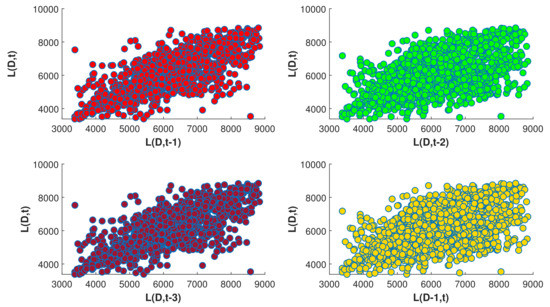
Figure 8. Impact of each input feature on output variable.

3. Results

Historical load data to train and test the models was considered from [28]. Date processing techniques for observing the data distribution and outliers and for data normalization have been used before using this data to train and test the regression model. Stochastic gradient descent optimizer has been used train the proposed regression models. The proposed regression models have been implemented and tested in cloud computing environment using Microsoft Azure Notebook [29].

3.1. Simple Linear Regression

A total of 2160 samples have been considered in the dataset; out of these, 1728 samples have been used for training and the remaining 432 samples have been used for testing.

3.1.1. Data Analysis

Statistical information of the active power load dataset is presented in Table 2. Scattering of data available in the dataset is presented in Figure 9. From the data scattering it has been observed that linear regression model can predict the load with good accuracy.

Table 2. SLR: statistical information of active power load dataset.

Parameter	Input	Output
count	2160	2160
mean	6037	6028
std	1066	1068
min	3378	3378
25%	5263	5260
50%	5950	5935
75%	6747	6739
max	8842	8842

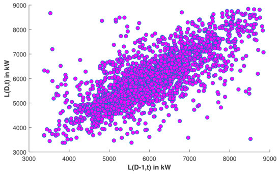
Figure 9. SLR: Scattering of data available in the dataset.

Box plot and histogram plot have been used to observe the input and output data distribution. Input and output data histograms are presented in Figure 10, and it has been observed that both input and output data samples follow the normal distribution.

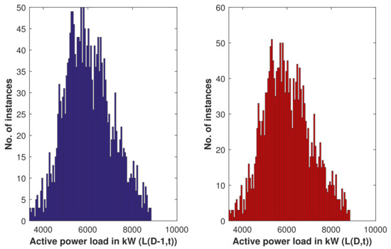
Figure 10. SLR: Data observation using histogram plot.

The box plot shown in Figure 11 is used to identify the outliers in the data and confirms that there are no outliers in the active power load dataset.

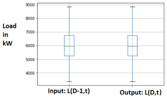
Figure 11. SLR: Data observation using box plot.

3.1.2. Simple Regression Model Performance Analysis

SLR model was trained with 1728 load data samples to find the optimum m and c values such that half mean distance from actual load data points to the line represented by optimum m and c values. The optimum m and c values after training using stochastic gradient descent optimizer are $0.7472$ and $0.1173$ respectively. The training performance of the model was measured in terms of MAE, MSE and RMSE and the respective values are $0.0973$, $0.01742$ and $0.132$.

The distribution of actual load $Y_a$ and load predicted using Equation (1) with training load data samples is presented in Figure 12 and similarly distribution of actual load $Y_a$ and predicted load with testing load data samples is presented in Figure 13.

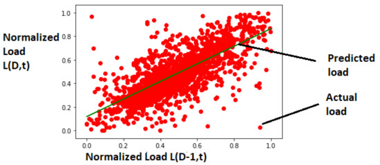
Figure 12. SLR: Distribution of actual load $Y_a$ and predicted load with training dataset and with m = 0.7472 and c = 0.1173.

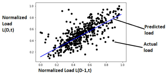
Figure 13. SLR: Distribution of actual load $Y_a$ and predicted load with testing dataset and with m = 0.7472 and c = 0.1173.

The performance of the model was observed using MAE, MSE and RMSE and the respective values with testing dataset were 0.0939, 0.0163 and 0.1277. The comparison of actual load available in testing dataset and load predicted with trained SLR model is presented in Figure 14.

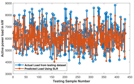
Figure 14. SLR: Comparison of actual load and predicted load with trained SLR model.

3.2. Multiple Linear Regression

A total of 2160 samples have been considered in the dataset; out of these, 1728 samples have been used for training and the remaining 432 samples have been used for testing of MLR model.

3.2.1. Data Analysis

Statistical information in terms of mean, standard deviation and inter quartile range of the active power load dataset is presented in Table 3. Dataset contains a total of four input parameters L(D,t−1), L(D,t−2), L(D,t−3) and L(D−1,t) and one output parameter L(D,t).

Table 3. MLR: Statistical information of active power load dataset.

Parameter	L(D,t−1)	L(D,t−2)	L(D,t−3)	L(D−1,t)	L(D,t)
count	2160	2160	2160	2160	2160
mean	6028	6028	6029	6037	6028
std	1068	1068	1068	1066	1068
min	3378	3378	3378	3378	3378
25%	5260	5260	5260	5263	5260
50%	5933	5935	5936	5950	5935
75%	6739	6739	6739	6747	6739
max	8842	8842	8842	8842	8842

Box plot and histogram plot have been used to observe the input and output data distribution. Input and output data histograms are presented in Figure 15, and it has been observed that both input and output data samples follow the normal distribution.

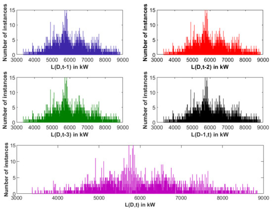
Figure 15. MLR: Data observation using histogram plot.

The box plot shown in Figure 16 is used to identify the abnormal data samples and it confirms that there are no outliers in the active power load dataset for MLR model.

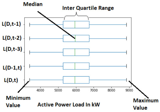
Figure 16. MLR: Data observation using box plot.

3.2.2. Multiple Regression Model Performance Analysis

MLR model was trained with 1728 load data samples to find the optimum $m_4$, $m_3$, $m_2$, $m_1$, and c values such that half mean distance from actual load data points to the line represented by optimum $m_1$, $m_2$, $m_3$, $m_4$ and c values. The optimum $m_1$, $m_2$, $m_3$, $m_4$ and c values after training using stochastic gradient descent optimizer are presented in Table 4. It has been observed that load at one hour before and one day before has positive and high impact on the predicted load. Similarly, load at two and three hours before has negative and low impact on the predicted load. The training performance of the MLR model was measured in terms of MAE, MSE and RMSE and the respective values are 0.0723, 0.0105 and 0.1026.

Table 4. MLR: coefficients and intercept information.

${\mathit{m}}_1$	${\mathit{m}}_2$	${\mathit{m}}_3$	${\mathit{m}}_4$	c
0.618733	−0.00289	−0.148361	0.374255	0.07541947

The performance of the model was observed using MAE, MSE and RMSE and the respective values with testing dataset were 0.0766, 0.0119 and 0.1092. The comparison of actual load available in testing dataset and load predicted with trained MLR model is presented in Figure 17.

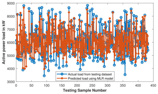
Figure 17. MLR: comparison of actual load and predicted load with trained MLR model.

3.2.3. MLR with Dimensionality Reduction (DR)

In MLR model load at particular hour (t) of the day (D) i.e., L(D,t) was predicted based on load data on last three hours from time of predicting and load at 24 h before. This means that a total of four input features were considered. Correlation among four input features were computed and presented in Table 5 and this information was used for dimensionality reduction, i.e., to reduce the number of input features and complexity of the model. As presented in Table 5, L(D,t−2) and L(D,t−3) have more than 75% correlation with L(D,t−1) and L(D,t−2), respectively. Hence feature L(D,t−2) was removed from input features and only L(D,t−1), L(D,t−3) and L(D−1,t) were considered as input features to predict the load L(D,t) using MLR model.

Table 5. MLR: coefficients and intercept information.

Features	L(D,t−1)	L(D,t−2)	L(D,t−3)	L(D−1,t)
L(D,t−1)	1	0.783398	0.547211	0.660699
L(D,t−2)	0.783398	1	0.783336	0.472053
L(D,t−3)	0.547211	0.783336	1	0.256744
L(D−1,t)	0.660699	0.472053	0.256744	1

MLR model was trained with 1728 load data samples having three input features, i.e., L(D,t−1), L(D,t−3) and L(D−1,t) to predict the load L(D,t). The optimum $m_1$, $m_2$, $m_3$ and c values after training using stochastic gradient descent optimizer are presented in Table 6. It has been observed that load at one hour before and one day before has positive and high impact on the predicted load. Similarly, load three hours before has negative and low impact on the predicted load.

Table 6. MLR with dimensionality reduction: coefficients and intercept information.

${\mathit{m}}_1$	${\mathit{m}}_2$	${\mathit{m}}_3$	c
0.596832	−0.137541	0.392209	0.07235393

The behavior of the MLR model prior to and after feature reduction was presented in Table 7. The behavior of the model was almost similar prior to and after dimensionality reduction in terms of error metrics.

Table 7. MLR with dimensionality reduction: performance of the model on training dataset.

	MAE	MSE	RMSE
With DR	0.0748	0.0113	0.107
Without DR	0.0723	0.0105	0.103

The behavior of the model with dimensionality reduction was compared with the behavior of the model without dimensionality reduction in terms of MAE, MSE and RMSE on testing dataset as presented in Table 8. The performance of the model was increased after applying the dimensionality reduction. It was happened due to removal of over fitting problem by reducing the number of input features and complexity of the model. The comparison of actual load available in testing dataset and load predicted with trained MLR model after reducing number of input features is presented in Figure 18.

Table 8. MLR with dimensionality reduction: performance of the model on testing dataset.

	MAE	MSE	RMSE
With DR	0.0679	0.009	0.093
Without DR	0.0766	0.0119	0.109

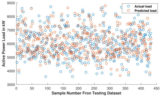
Figure 18. MLR With Dimensionality Reduction: comparison of actual load and predicted load with trained MLR model.

3.3. Polynomial Regression Model

A total of 2160 samples have been considered in the dataset; out of these, 1728 samples have been used for training and the remaining 432 samples have been used for testing of the PR model. The approach used for PR model is prediction of load at a particular hour of the day based on load at 24 h before, which is similar to the approach which was used for SLR. The same dataset was used for both simple and PR models.

PR Model Performance Analysis

PR model with different degree of polynomial (p) was trained with 1728 load data samples to find the optimum $m_i$ where i $ϵ$ {1,2,...,p} and c values so that half mean distance from actual load data points to the curve represented by optimum $m_i$ and c values was minimum. Optimum $m_i$ and c values for different degree of PR models were presented in Table 9.

Table 9. PR: coefficients and intercept information.

Degree (p)	${\mathit{m}}_1$	${\mathit{m}}_2$	${\mathit{m}}_3$	${\mathit{m}}_4$	${\mathit{m}}_5$	${\mathit{m}}_6$	${\mathit{m}}_7$	${\mathit{m}}_8$
2	0.6061	0.1345	NA	NA	NA	NA	NA	NA
3	−0.016	1.5525	−0.936	NA	NA	NA	NA	NA
4	−0.235	2.4303	−2.25139	0.65556	NA	NA	NA	NA
5	−1.458	9.886	−20.92	21.1449	−8.156	NA	NA	NA
10	3.8512	−90.59	857.68	−3885.2	10,407	17,572.45	19067.9	13006.7
15	20.437	−802.9	13357	−121,706	661,929	−2,132,575	3,267,138	2,932,709
Degree (p)	${\mathit{m}}_{\mathbf{9}}$	${\mathit{m}}_{\mathbf{10}}$	${\mathit{m}}_{\mathbf{11}}$	${\mathit{m}}_{\mathbf{12}}$	${\mathit{m}}_{\mathbf{13}}$	${\mathit{m}}_{\mathbf{14}}$	${\mathit{m}}_{\mathbf{15}}$	c
2	NA	NA	NA	NA	NA	NA	NA	0.15478
3	NA	NA	NA	NA	NA	NA	NA	0.22922
4	NA	NA	NA	NA	NA	NA	NA	0.24466
5	NA	NA	NA	NA	NA	NA	NA	0.30014
10	5113.5	-888.6	NA	NA	NA	NA	NA	0.25182
15	−3 × 10${}^7$	7 × 10${}^7$	−1 × 10${}^8$	9.2 × 10${}^7$	−5 × 10${}^7$	18132030	−3 × 10${}^6$	0.19706

The training of various PR models has been observed in terms of MAE, MSE and RMSE. Table 10 presents MAE, MSE and RMSE values during training for different PR models. It has been observed from Table 10 that the training performance metrics values, i.e., MAE, MSE and RMSE values decrease by increasing the degree of polynomial. This means that the training performance of the model is increasing with the degree of polynomial.

Table 10. PR: training performance metrics.

Polynomial Degree (p)	Training
	MAE	MSE	RMSE
3	0.0973329	0.01732	0.131609177
4	0.0973174	0.01732	0.131591693
10	0.0970367	0.01717	0.131019329
15	0.0969165	0.01708	0.130697822
16	0.0968882	0.01708	0.130688064
18	0.0969342	0.01707	0.130644772
20	0.0970481	0.01705	0.130574147

The actual performance of various PR models has been observed with testing data and presented in Table 11. The performance metrics’ values have been observed, i.e., MSE and RMSE values decrease up to the degree of polynomial 15 and beyond that increase. This means that if testing performance of the model increases with degree of polynomial up to 15 and beyond that decreases, it is due to overfitting of the model.

Table 11. PR: testing performance metrics.

Polynomial Degree (p)	Training
	MAE	MSE	RMSE
3	0.09289	0.015969	0.12637
4	0.09276	0.015939	0.12625
10	0.09274	0.015889	0.12605
15	0.09295	0.015849	0.12589
16	0.09292	0.015853	0.12591
18	0.09308	0.015877	0.12600
20	0.09311	0.015900	0.12609

Figure 19 shows the variation of RMSE value of model with degree of polynomial on both training and testing dataset. It has been observed from the Figure 19 that training performance of the model increases with degree of polynomial. However, testing performance of the model increases with polynomial degree up to 15 but beyond that testing performance decreases due to overfitting problem. Hence, PR model with degree 15 is considered as the optimal model to deploy.

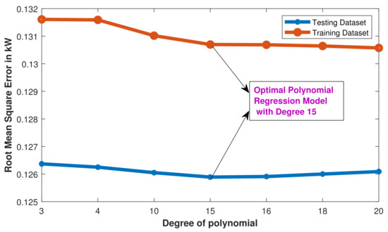
Figure 19. PR: identification of Optimal PR Model.

The comparison of actual load available in testing dataset and the load predicted with trained PR model having polynomial degree 15 is presented in Figure 20. It has been observed that most of the predicted load points are close to the actual load.

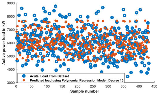
Figure 20. PR: comparison of actual load and predicted load with trained PR model.

3.4. Comparative Analysis

The proposed SLR model, MLR model with and without DR and PR model to predict the load on a 33/11 kV substation were compared in terms of MAE, MSE and RMSE as shown in Table 12. It has been observed that MLR model with DR has low MAE, MSE and RMSE values compared to simple linear and multiple linear without DR and PR models. Which means that MLR model with DR predicted the load with good accuracy compared to simple linear and multiple linear without DR and PR models.

Table 12. Comparison of regression models’ performance on testing dataset.

Regression
Model	MAE	MSE	RMSE
SLR	0.0939	0.0163	0.1277
PR	0.0930	0.0158	0.1259
MLR	0.0766	0.0119	0.1092
MLR with DR	0.0679	0.009	0.093

The load on a substation varied from 3 MW to 9 MW during the observation period, and building a regression model by considering +/−0.5 MW load variation can be significant. The number of times each model failed to predict below the threshold limit is shown in Figure 21.

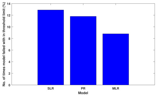
Figure 21. Model performance to predict load with in threshold limit.

The performance of the proposed models was compared with existing models available in the literature [17,18] in terms of training and testing MSE and presented in Table 13. The proposed multiple linear regression (MLR) with dimensionality reduction performs well with low mean square error 0.009 over the existing models.

Table 13. Performance comparison with existing complex models.

	Mean Square Error
Model	Training	Testing
SLR	0.0973	0.0163
PR	0.0171	0.0158
MLR	0.0723	0.0119
MLR with DR	0.0748	0.009
[18]	0.23	0.44
[17]	0.29	1.59

In comparison with other techniques, the proposed regression models stand out on the data considered for the discussed problem in terms of speed due to light weight models, accuracy due to a suitable model chosen based on data distribution and simplicity due to a very simple model with 2 model parameters for SLR, 16 model parameters for PR and 5 model parameters for multi-variable linear regression model.

4. Conclusions

The SLR, MLR and PR models were used in this paper to estimate the active power load on a 33/11 kV substation. Dimensionality reduction based on correlation among MLR model input features was used to reduce the model’s complexity and overfitting issue.

The analytical results indicate that the proposed regression models predicts active power load with good accuracy. The analytical results concluded that the proposed MLR model with dimensionality reduction performs better. This paper offers a detailed tool for network operators to efficiently exchange energy and run the network.

The methodology to predict load using regression models can be applied to other power system research areas such as LMP computation, effective trading in the energy market, power system deregulation and so on. This load prediction work can be expanded by taking into account sequential networks as well as weekdays and weekends.

References

- Almeshaiei, E.; Soltan, H. A methodology for electric power load forecasting. Alex. Eng. J. 2011, 50, 137–144. [Google Scholar] [CrossRef]
- Foldvik Eikeland, O.; Bianchi, F.M.; Apostoleris, H.; Hansen, M.; Chiou, Y.C.; Chiesa, M. Predicting Energy Demand in Semi-Remote Arctic Locations. Energies 2021, 14, 798. [Google Scholar] [CrossRef]
- Alam, S.; Ali, M. Equation Based New Methods for Residential Load Forecasting. Energies 2020, 13, 6378. [Google Scholar] [CrossRef]
- Mi, J.; Fan, L.; Duan, X.; Qiu, Y. Short-term power load forecasting method based on improved exponential smoothing grey model. Math. Probl. Eng. 2018, 2018. [Google Scholar] [CrossRef]
- Hu, R.; Wen, S.; Zeng, Z.; Huang, T. A short-term power load forecasting model based on the generalized regression neural network with decreasing step fruit fly optimization algorithm. Neurocomputing 2017, 221, 24–31. [Google Scholar] [CrossRef]
- Kumar, B.A.; Sangeetha, G.; Srinivas, A.; Awoyera, P.; Gobinath, R.; Ramana, V.V. Models for Predictions of Mechanical Properties of Low-Density Self-compacting Concrete Prepared from Mineral Admixtures and Pumice Stone. In Soft Computing for Problem Solving; Springer: New York, NY, USA, 2020; pp. 677–690. [Google Scholar]
- Awoyera, P.; Akinmusuru, J.; Krishna, A.S.; Gobinath, R.; Arunkumar, B.; Sangeetha, G. Model Development for Strength Properties of Laterized Concrete Using Artificial Neural Network Principles. In Soft Computing for Problem Solving; Springer: New York, NY, USA, 2020; pp. 197–207. [Google Scholar]
- Veeramsetty, V.; Singal, G.; Badal, T. Coinnet: Platform independent application to recognize Indian currency notes using deep learning techniques. Multimed. Tools Appl. 2020, 79, 22569–22594. [Google Scholar] [CrossRef]
- Bassi, S.; Gomekar, A.; Murthy, A.V. A learning algorithm for time series based on statistical features. Int. J. Adv. Eng. Sci. Appl. Math. 2019, 11, 230–235. [Google Scholar] [CrossRef]
- Lakshmi, G.N.; Jayalaxmi, A.; Veeramsetty, V. Optimal placement of distributed generation using firefly algorithm. In IOP Conference Series: Materials Science and Engineering; IOP Publishing: Bristol, UK, 2020; Volume 981, p. 042060. [Google Scholar]
- Veeramsetty, V.; Chintham, V.; D.M., V.K. Locational marginal price computation in radial distribution system using Self Adaptive Levy Flight based JAYA Algorithm and game theory. Int. J. Emerg. Electr. Power Syst. 2021, 22, 215–231. [Google Scholar]
- Ali, M.; Iqbal, M.J.; Sharif, M. Relationship between extreme temperature and electricity demand in Pakistan. Int. J. Energy Environ. Eng. 2013, 4, 36. [Google Scholar] [CrossRef]
- Mirmasoudi, S.; Byrne, J.; Kroebel, R.; Johnson, D.; MacDonald, R. A novel time-effective model for daily distributed solar radiation estimates across variable terrain. Int. J. Energy Environ. Eng. 2018, 9, 383–398. [Google Scholar] [CrossRef]
- Panapakidis, I.P.; Dagoumas, A.S. Day-ahead electricity price forecasting via the application of artificial neural network based models. Appl. Energy 2016, 172, 132–151. [Google Scholar] [CrossRef]
- Amral, N.; Ozveren, C.; King, D. Short term load forecasting using multiple linear regression. In Proceedings of the 2007 42nd International Universities Power Engineering Conference, Brighton, UK, 4–6 September 2007; pp. 1192–1198. [Google Scholar]
- Kumar, S.; Mishra, S.; Gupta, S. Short term load forecasting using ANN and multiple linear regression. In Proceedings of the 2016 Second International Conference on Computational Intelligence & Communication Technology (CICT), Ghaziabad, India, 12–13 February 2016; pp. 184–186. [Google Scholar]
- Shaloudegi, K.; Madinehi, N.; Hosseinian, S.; Abyaneh, H.A. A novel policy for locational marginal price calculation in distribution systems based on loss reduction allocation using game theory. IEEE Trans. Power Syst. 2012, 27, 811–820. [Google Scholar] [CrossRef]
- Veeramsetty, V.; Chintham, V.; Vinod Kumar, D. Proportional nucleolus game theory–based locational marginal price computation for loss and emission reduction in a radial distribution system. Int. Trans. Electr. Energy Syst. 2018, 28, e2573. [Google Scholar] [CrossRef]
- Veeramsetty, V.; Chintham, V.; DM, V.K. LMP computation at DG buses in radial distribution system. Int. J. Energy Sect. Manag. 2018, 12, 364–385. [Google Scholar] [CrossRef]
- Veeramsetty, V.; Deshmukh, R. Electric power load forecasting on a 33/11 kV substation using artificial neural networks. SN Appl. Sci. 2020, 2, 855. [Google Scholar] [CrossRef]
- Houimli, R.; Zmami, M.; Ben-Salha, O. Short-term electric load forecasting in Tunisia using artificial neural networks. Energy Syst. 2019, 11, 357–375. [Google Scholar] [CrossRef]
- Lisi, F.; Shah, I. Forecasting next-day electricity demand and prices based on functional models. Energy Syst. 2019, 11, 947–979. [Google Scholar] [CrossRef]
- Li, K.; Zhang, T. A novel grey forecasting model and its application in forecasting the energy consumption in Shanghai. Energy Syst. 2019, 12, 357–372. [Google Scholar] [CrossRef]
- Shamir, O.; Zhang, T. Stochastic gradient descent for non-smooth optimization: Convergence results and optimal averaging schemes. In Proceedings of the 30th International Conference on Machine Learning, Atlanta, GA, USA, 16–21 June 2013; pp. 71–79. [Google Scholar]
- Parol, M.; Piotrowski, P.; Kapler, P.; Piotrowski, M. Forecasting of 10-Second Power Demand of Highly Variable Loads for Microgrid Operation Control. Energies 2021, 14, 1290. [Google Scholar] [CrossRef]
- Zheng, J.; Zhang, L.; Chen, J.; Wu, G.; Ni, S.; Hu, Z.; Weng, C.; Chen, Z. Multiple-Load Forecasting for Integrated Energy System Based on Copula-DBiLSTM. Energies 2021, 14, 2188. [Google Scholar] [CrossRef]
- Jin, X.B.; Zheng, W.Z.; Kong, J.L.; Wang, X.Y.; Bai, Y.T.; Su, T.L.; Lin, S. Deep-Learning Forecasting Method for Electric Power Load via Attention-Based Encoder-Decoder with Bayesian Optimization. Energies 2021, 14, 1596. [Google Scholar] [CrossRef]
- Venkataramana, V. Active Power Load Dataset. 2020. Available online: http://dx.doi.org/10.17632/ycfwwyyx7d.2 (accessed on 19 May 2021).
- Barga, R.; Fontama, V.; Tok, W.H.; Cabrera-Cordon, L. Predictive Analytics with Microsoft Azure Machine Learning; Springer: New York, NY, USA, 2015. [Google Scholar]
Publisher’s Note: MDPI stays neutral with regard to jurisdictional claims in published maps and institutional affiliations. |
© 2021 by the authors. Licensee MDPI, Basel, Switzerland. This article is an open access article distributed under the terms and conditions of the Creative Commons Attribution (CC BY) license (https://creativecommons.org/licenses/by/4.0/).