Battery-Aware Electric Truck Delivery Route Exploration ^†

Abstract

The energy-optimal routing of Electric Vehicles (EVs) in the context of parcel delivery is more complicated than for conventional Internal Combustion Engine (ICE) vehicles, in which the total travel distance is the most critical metric. The total energy consumption of EV delivery strongly depends on the order of delivery because of transported parcel weight changing over time, which directly affects the battery efficiency. Therefore, it is not suitable to find an optimal routing solution with traditional routing algorithms such as the Traveling Salesman Problem (TSP), which use a static quantity (e.g., distance) as a metric. In this paper, we explore appropriate metrics considering the varying transported parcel total weight and achieve a solution for the least-energy delivery problem using EVs. We implement an electric truck simulator based on EV powertrain model and nonlinear battery model. We evaluate different metrics to assess their quality on small size instances for which the optimal solution can be computed exhaustively. A greedy algorithm using the empirically best metric (namely, distance × residual weight) provides significant reductions (up to 33%) with respect to a common-sense heaviest first package delivery route determined using a metric suggested by the battery properties. This algorithm also outperforms the state-of-the-art TSP heuristic algorithms, which consumes up to 12.46% more energy and 8.6 times more runtime. We also estimate how the proposed algorithms work well on real roads interconnecting cities located at different altitudes as a case study.

1. Introduction

Electric Vehicles (EVs) are currently a tiny fraction of the car market, which is dominated by Internal Combustion Engine Vehicles (ICEVs); however, the growth of the EV market over last ten years is remarkable, and they are expected to progressively replace ICEVs in the next 20 years.

EVs have high energy efficiency and are sustainable transportation, since their electric motor has high dynamic performance and they are more environmentally-friendly than ICEVs on the market today; even when evaluating the emissions generated during electricity production for the charge of EVs, their overall Greenhouse Gas (GHG) emission is up to 58% that lower than the emissions of average mid-size passenger ICEVs [1]. Moreover, the impact on climate change by the production of electricity and operation of EVs is up to 30% less compared with ICEVs when considering the average generation of electricity in Europe. In recent years, the landscape of EVs is widening and expands to domains such as electric racing cars, electric buses, and electric trucks.

In particular, Tesla announced electric trucks will replace existing ICE trucks in the future [2]. The electric truck can accelerate more quickly than conventional diesel trucks because of the characteristic of the electric motor: high torque at low Rotations Per Minute (RPM) with high efficient. Furthermore, 98% of the kinetic energy can be recovered with electric energy during regenerative braking, which makes the electric truck more energy efficient. According to the announcement by Tesla, electric truck owners can save more than $200,000 over a million miles compared to fuel cost of a conventional truck.

The optimal energy-efficient delivery route can further improve the energy efficient of electric trucks. The typical delivery scenario is defined as an electric truck loads all packages for customers at a depot, visits each customer to deliver their package, and then returns to the depot without payload. For a conventional ICEV, the “cost” of a path is strongly driven by the distance (even if weight also matters) and the problem nicely fits into the well-known Traveling Salesman Problem (TSP) using distance as a metric. However, when considering EVs, the solution is not as straightforward; although distance obviously matters, the total energy consumption also strongly depends on the order of delivery as the efficiency of the EV is affected by the total (vehicle + payload) weight. Since the impact of the package weight on the battery SOC of electric trucks is much higher than that of the ICE trucks due to the characteristics of battery, the energy-optimal delivery method for electric trucks should be newly considered. As a matter of fact, one key characteristic of a battery is that it is progressively less efficient in delivering its energy as its State Of Charge (SOC) decreases [3,4]. A fully charged lithium-ion battery in EVs has better performance to deliver a high power demand than when it is partially discharged [5]. As the power consumption of the electrical motor strongly depends on the total weight, apparently, if we deliver the heaviest package first, the overall vehicle weight is reduced the most after unloading this package and following such order would be optimal [5]. On the other hand, it is obvious that the delivery distance should be considered; if we deliver the heaviest package first and this package has a very long distance from the depot, the battery will be discharged by carrying the heaviest weight for a long time, which might lead to a non-optimal delivery route if following the rule of deliver heaviest package first.

One first difference with respect to a plain ICEVs delivery is therefore in terms of metrics: for EVs, some combination of weight and distance should be considered. However, the most significant difference (and complication) lies in the fact that the calculation of the optimal energy path cannot be done incrementally, as the energy cost of a path is “dynamic”, i.e., it depends on the previous choices as a consequence of the dependence on the residual weight, which means the weight and distance are the variables during the delivery process.

In this paper, we propose an overall electric trucks delivery simulation framework implemented by SystemC and SystemC-AMS for the least-energy electric truck delivery routing problem. We first implement an electric truck simulator with a powertrain model and a non-linear battery model of the Tesla Semi [6] that adopts the methodology introduced in [3] to trace the SOC evolution during the package delivery. From the simulation results, we show that a conventional metric for TSP, total delivery distance, as with any other “static” metric, does not minimize total energy consumption for an EV delivery. Since only an exhaustive exploration of all path guarantees to find the optimal path, we evaluate different static metrics (functions of weight and distance) on small graph instances to assess their quality; then, using the best metric derived in this calibration phase, we show how a greedy algorithm using that metric can provide significant reductions (up to 33%) with respect to the common-sense heaviest first package delivery.

The work is an extension of our previous conference paper [7], the main contribution of this work is to devise a heuristic algorithm to determine the energy-optimal routing of an electric truck. This main results encompasses a number of elements that we summarize as follows:

• Implement an electric truck simulator with a powertrain model and a non-linear battery model.
• Explore all delivery paths and evaluate the the correlation between energy consumption and various delivery metrics.
• Introduce heuristic algorithms using the best metrics, and show simulation results providing significant reductions of energy consumption.
• Analyze the effects of package weight distribution and number of packages on energy saving.
• Perform the proposed routing methods on the real routing condition, which consider average road speed, road distance between cities and corresponding road slope.

The paper is organized as follows. Section 2 introduces the motivation for the least-energy electric truck delivery routing problem. A comparison between the traditional shortest distance route and heaviest first route presented in this section to illustrate the limitation of distance-based routing method for the electric truck delivery routing problem. Section 3 describes the EV powertrain model and battery model used in our simulation framework and the typical vehicle routing problem. Section 4 shows our analysis of the routing problem; we discuss new metric candidates considering both of delivery distance and package weight. Then, new heuristic methods are proposed including greedy algorithm and TSP methods. Section 5 firstly shows how to implement the powertrain model of an electric truck and the related battery model in our simulation; then, the model validation follows. After that, we compare the energy consumption for the electric truck delivery problem by the metrics and approximate algorithms. To evaluate our proposal in the real delivery environment, we performed a case study for the delivery in a province located in Italy. Finally, Section 6 gives the conclusion of our work.

2. Motivation

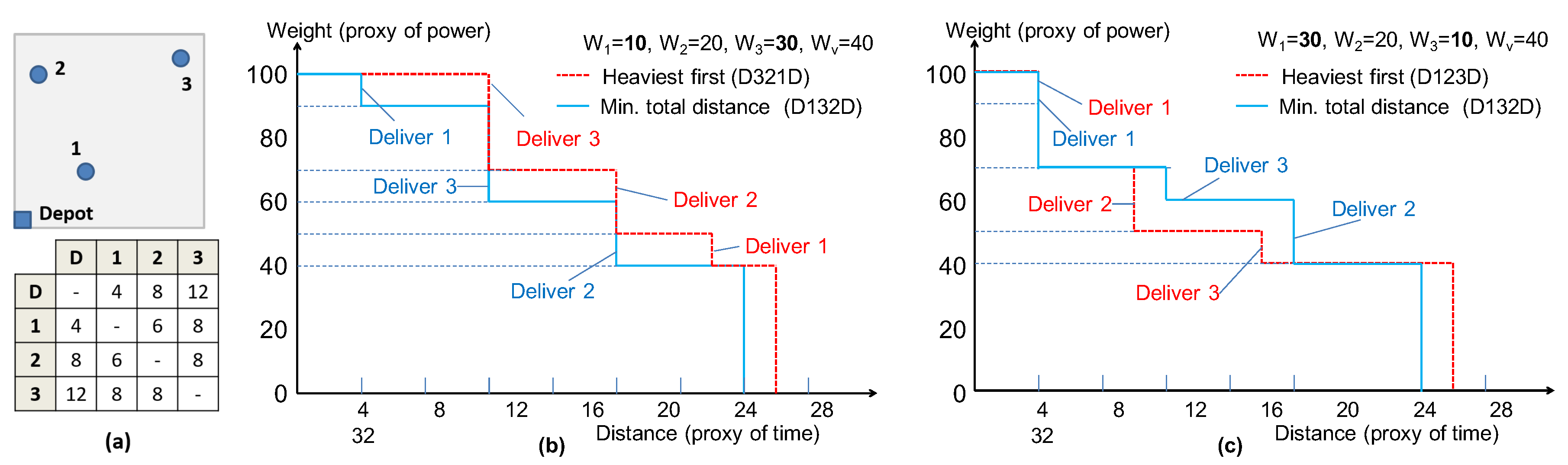
In order to clearly illustrate the motivation of this work, we built an example to indicate how it is not possible to derive an energy-optimal delivery policy simply using a single “static” metric. Figure 1a shows a simple three-destinational delivery task from a depot (D) with a rough mapping on the plane, and the distance matrix between any pair of destinations. We assumed symmetry between node pairs to guarantee the generality.

Figure 1. Example to illustrate the motivation of energy-optimal delivery route exploration cannot only depend on single static metric: a delivery task (a) and delivery routes for two different delivery weights (b,c).

To evaluate the energy cost of a delivery path, we use a time diagram that plots the evolution of the total transported weight over delivery distance. We use weight as a proxy of electric truck power consumption, since it is proportional to the weight of the vehicle plus the total payload. Notice that it is clearly a simplification and does not take into account non-linearities of a battery, but even such approximation can help reveal the point we are making.

Distance is used as a proxy of time; we assume a constant speed for the deliveries. Again, this is an approximation of the real setting, where speed can be extremely varying due to the driving habits and the road traffic. When using a real battery model in the loop, however, the real speed profile of the vehicle can be accounted for. Therefore, evolution of weight over distance is a proxy of power over time, and the area of one such curve is then an estimate of the energy consumed for that delivery route.

Figure 1b shows two such delivery routes for a case in which the weights are $W_1=10,W_2=20,W_3=30$ and vehicle weight is $W_v=40$. The dotted red curve represents a route for which packages are delivered in heaviest-first order ($D\to 3\to 2\to 1\to D$), whereas the solid blue line denotes a route with the minimum total distance ($D\to 1\to 3\to 2\to D$). In this specific case, the “min. total distance” policy works best (smaller area under the curve) and, by exhaustive exploration of the 3!=6 combinations of deliveries, it can be shown to yield the best value of the metric. Notice that the ($D\to 3\to 2\to 1\to D$) route is not just slightly sub-optimal, and it ranks fourth out of the six routes, $D\to 3\to 1\to 2\to D$ being the worst one.

Figure 1c shows two other waveforms for the same delivery task in which the weights change to $W_1=30,W_2=20,W_3=10$, that is, in which the heaviest package corresponds to the closest destination (node 1). In this case, the red dotted profile of the “heaviest-first” yields the best value of the metric, while the “min. total distance” yields a slightly worse value. Notice that the blue solid line corresponds to the same order of delivery (yet with a different cost) as in Figure 1b as the distance has not changed in the two examples.

Notice also that (due the symmetric distances) there are two paths (i.e., $D\to 1\to 3\to 2\to D$ and $D\to 2\to 3\to 1\to D$) with the same distance but with different “energy” cost, the cost of the path $D\to 2\to 3\to 1\to D$ being larger than the other one shown in Figure 1c. Therefore, an algorithm that picks edge simply based on distance could even get farther from the optimal solution.

In this straightforward example, although there are several approximations during the power consumption estimation, it shows the main two critical points raised by our work. Firstly, no simple single static metric can solve ideally the problem of searching the energy-optimal delivery route. Secondly, due to the state-dependent characteristic of the cost function, only the brutal exhaustive exploration can find the optimal solution, but, since this is only feasible for very small instances, we need to find a provably good static metric that can be used in a heuristic algorithm. According to the above finding from the motivating example, this static metric should combine both weight and distance as twinned factors affecting the energy consumption of the EV.

3. Background and Related Work

3.1. Powertrain Model in EV

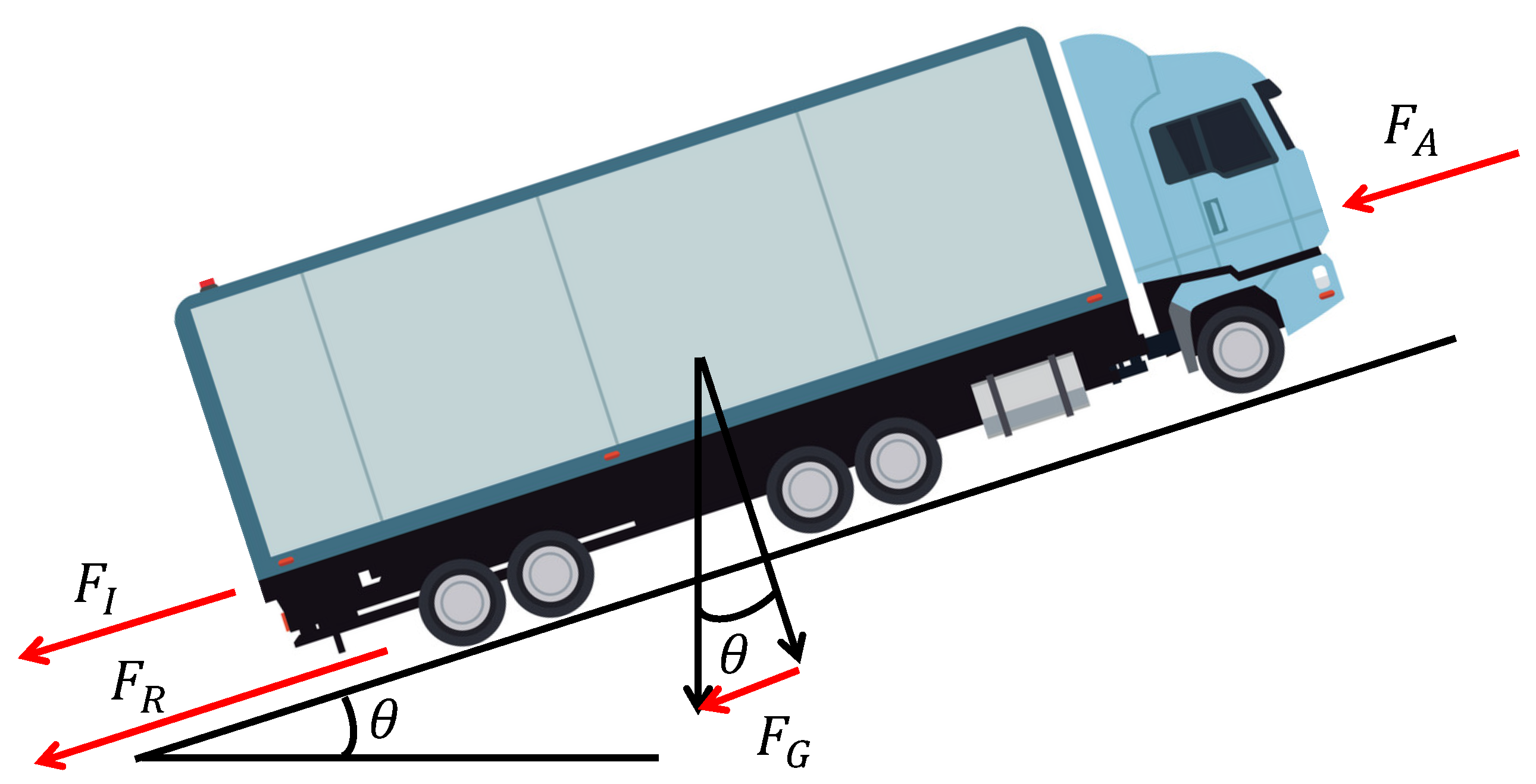
As is common, the vehicle powertrain model is from the vehicle dynamics. There are four forces acting on a vehicle driving on a road with $\theta$ road slope, as shown in Figure 2: rolling resistance $F_R$, gradient resistance $F_G$, inertia resistance $F_I$, and aerodynamic resistance $F_A$.

Figure 2. Forces acting on a truck.

The powertrain model by vehicle dynamics ($P_{dyna}$) is described as

$$\begin{array}{cc}\hfill P_{dyna}& =T\omega =F\frac{ds}{dt}=(F_R+F_G+F_I+F_A)v\hfill \\ \hfill F_R\propto C_{rr}W,F_G& \propto Wsin\theta ,F_I\propto ma,\mathrm{and} F_A\propto \frac{1}{2}\rho C_{d}A{v}^2\hfill \\ \hfill P_{dyna}& \approx (\alpha +\beta sin\theta +\gamma a+\delta v^2)mv\hfill \end{array}$$

(1)

where $C_{rr}$ is the rolling coefficient, W is vehicle weight, $\theta$ is road slope, m is vehicle mass, v is vehicle speed, a is vehicle acceleration, $C_d$ is drag coefficient, and A is the vehicle facial area [8]. The coefficients $\alpha ,\beta ,\gamma$, and $\delta$ of the dynamic power $P_{dyna}$ are coefficients of rolling resistance, gradient, inertia, and aerodynamic, respectively.

In addition to the forces, there are several losses on a rotating motor: a copper loss is proportional to the square of motor torque and iron and friction loss are related to motor RPM. In addition, there is a constant loss while the vehicle is operating. The powertrain model of EV ($P_{EV}$) includes the motor losses in addition to $P_{dyna}$:

$$P_{EV}=P_{dyna}+C_0+C_{1}v+C_2{v}^2+C_3{T}^2.$$

(2)

where $C_0$, $C_1$, $C_2$, and $C_3$ are the coefficients for constant loss, iron and friction loss, copper loss, and drivetrain loss, respectively.

EVs and hybrid vehicles mostly use regenerative braking during deceleration. The regenerative braking converts kinetic energy to electric energy from generation process. The harvested energy is related to the electromagnetic flux inside of the motor, which is proportional to the motor RPM. Therefore, the regenerative braking model can be simplified as

$$P_{regen}=ϵTv+\zeta .$$

(3)

where $ϵ$ and $\zeta$ are regenerative braking coefficients to model the regenerative power as a function of the current velocity.

3.2. Battery Model in EV

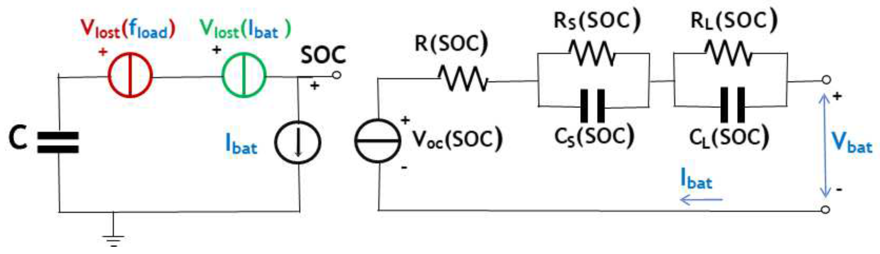
The EV is normally powered by a battery pack that includes a large number of Lithium battery cells connected in parallel and series. The battery pack of Tesla Model 3 with long range version comprises 4416 2170-size lithium-ion cells of 4800 mAh nominal capacity with 46p96s arrangement, and 800 km range. Tesla Semi truck has a 750 kWh battery pack and weighs about 5.1 tons. To build the battery pack model directly is a non-trivial task, therefore, the battery pack can be built by composing the individual battery cell model, and the model must be able to accurately account for the varied load current and SOC variations of the usable battery capacity to capture the non-ideal discharge characteristics of battery. We select a circuit-equivalent battery model that can model the effects of load current magnitude and dynamics on real-time battery usable capacity [9], and then use this model to compose the whole battery pack model.

Figure 3 depicts the circuit-equivalent model of one battery cell adopted in this work. The left-hand part for modeling the battery lifetime (usable capacity) and the the right-hand part represents the transient battery voltage. Notice that the left-hand part also account for current magnitude and load frequency dependency on actual battery capacity. The left-hand part comprises a capacitor C representing the nominal storage capacity of the battery in $Ah$ and a current generator representing the battery current $I_{batt}$ requested by the load. As the available capacity of the battery is affected by the load current variations distribution, there are two voltage generators on the left part: one represents the dependency of the battery capacity on the current values, while the other generator models the dependency on load current frequency. Both decrease the voltage at node SOC, representing the SOC, for larger current magnitudes and frequencies. The right-part has a variable voltage generator affected by the SOC of battery, the internal resistance is also influenced by the current SOC of battery, and two pairs of RC express the instantaneous battery voltage.

Figure 3. Adopted circuit-equivalent model for one single battery cell.

The methodology to extract the relationship between SOC and internal resistance, capacitance, and open circuit voltage is presented in [10], and the implementation of adding two different dependencies of load current on the left-hand side of model is introduced in [9].

Based on this single cell model, we derive the battery pack model by ideally scaling all electrical parameters according to the series/parallel configuration in the pack, which leads to faster simulation runs and a higher flexibility in the modeling of large battery pack, so that not all cells of a large pack have to be modeled and simulated individually. Notice that the implementation of battery pack model is somehow ideal (e.g., cell mismatches are not considered), while this is still more accurate than a linear battery model that neglects state-dependent battery characteristic.

Given this model, we can track the energy consumed by the EV by applying to the model the drawn power (as current and voltage waveforms) corresponding to the electrical motor consumption on a given leg of the route. In the most general case, there is a non-ideal power conversion step between the electrical motor and the battery. In this case, it suffices to scale the motor current and voltage according to the converter efficiency $\eta <1$, which can be any complex function of the motor parameters, i.e., $P_{batt}=P_{motor}·\eta$. We assume the converter efficiency is a fixed valued in this work as in [3].

3.3. Work Flow of Proposed Methodology

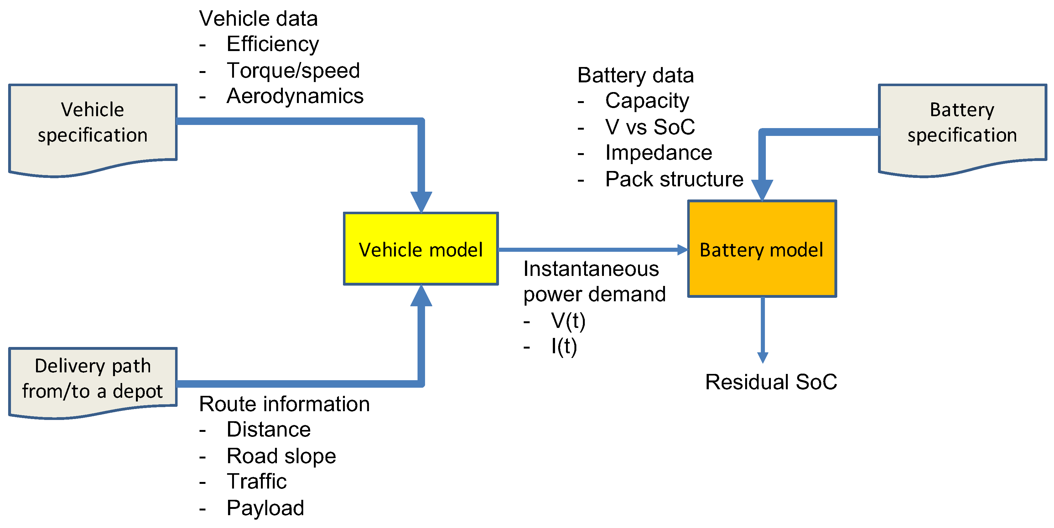
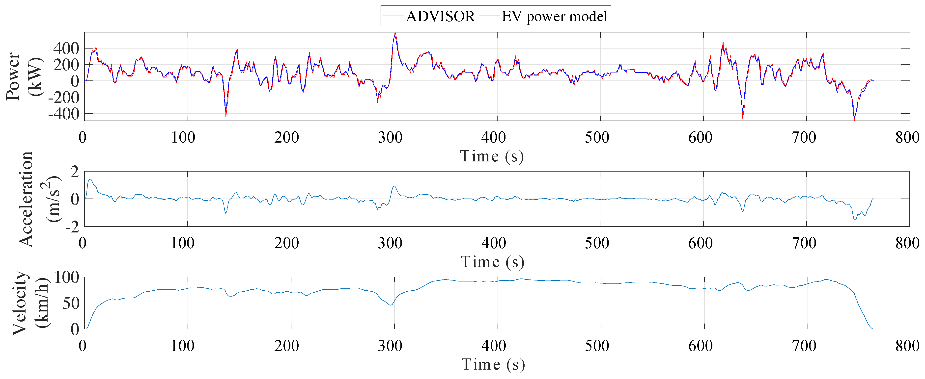
Figure 4 shows the conceptual flow of our methodology for the estimation of the operation range of EVs. Three descriptive datasets are required as inputs.

Figure 4. Overall concept of the proposed methodology.

Vehicle data includes (1) motor information: motor efficiency by motor torque and RPM, operation range of motor torque and RPM, (2) vehicle information: weight, drive train and body shape, and (3) other electrical systems. Facial area of the vehicle affects aerodynamic resistance. Route information include road distance between cities, road slope, and traffic on each road. Also payload by a delivery task is given. Route information and vehicle data is used in the vehicle model, which generates instantaneous power demand (V(t) and I(t)) during delivery.

We implement a battery model from a given battery specification: nominal capacity, voltage-to-SOC curve, impedance, and structure of the battery pack. Then we combine the vehicle model and battery model together to conduct simulation, the power demand of given delivery tasks over time derived from vehicle model is pass into battery model, finally the battery model computes the residual SOC of battery pack.

3.4. Vehicle Routing Problem

The vehicle routing problem is formulated as a graph $G(V,E,C)$ where $V=\{v_0,\cdots ,v_N\}$ is the set of vertices including N destinations and a depot, $E=\left\{e_{ij}{|}_{i,j\in V}\right\}$ is the set of edges between two vertices $v_i$ and $v_j$, and $C=\left\{c_{ij}{|}_{i,j\in V}\right\}$ is the cost related to each edge $e_{ij}$. Vertex $v_0$ is the depot, while the remaining vertices in V represent customers that need to be served. The TSP consists in finding a route based at the depot, such that each of the vertices is visited exactly once while minimizing the overall routing cost.

The formulation of the vehicle routing problem is generalized as the TSP. Because TSP is known as NP-hard, several approximation algorithms are proposed during last several decades. Christofides designed an approximation algorithm for TSP using the Minimum Spanning Tree (MST) algorithm, which obtains approximated results less than 1.5 times the optimal solution [11]. From the general TSP, there are several variants of TSP to consider various constraints and delivery requirements. There is a variant of TSP considering a set of potential customers living near secured customers [12]. The salesman finds the shortest path to cover all potential customers within a certain distance from the path. A fleet of delivery vehicles characterized by different capacities and costs is an important variant of TSP [13,14]. There is a set of customers and a set of different types of vehicles. Each vehicle has different capacities in terms of the number of customers and operation cost; the goal is to find a set of routes for each vehicle minimizing total delivery cost. Some studies consider the number of customers that each vehicle should be responsible for, but they do not consider the vehicle weight changing with each delivery.

Recently, the vehicle routing problem with pick-up and delivery considers the situation in which packages have to be picked-up from one of customers and delivered to another location [15,16]. During the pick-up and delivery process, visiting each pickup and delivery places occurs exactly once and total package weight during the delivery should not exceed the capacity. This problem considers the weight of each package; however, it does not consider the energy consumption that changes after unloading each package.

There is a paper minimizing energy in the vehicle routing problem [17]. This paper solves the vehicle routing problem using integer linear programming to minimize the product of distance and weight of each arc. However, there is no result validation using energy simulation. Therefore, there is no analysis of energy consumption in the points of view of package weight distribution and routing methods in the real road condition.

4. Analysis of Routing Algorithms

The examples in Figure 1 suggest that a reasonable metric to track the energy spent on a delivery path could be to use a quantity that is correlated to the product of distance × weight. More precisely, let i and j be two vertices of the delivery graph, $d_{ij}$ the distance between them, and $W_i$ and $W_j$ the weights to be delivered, respectively, at i and j. This metric should be proportional to $d_{ij}\times (W_{current}-W_i)$, assuming the edge is traveled in the direction $i\to j$. 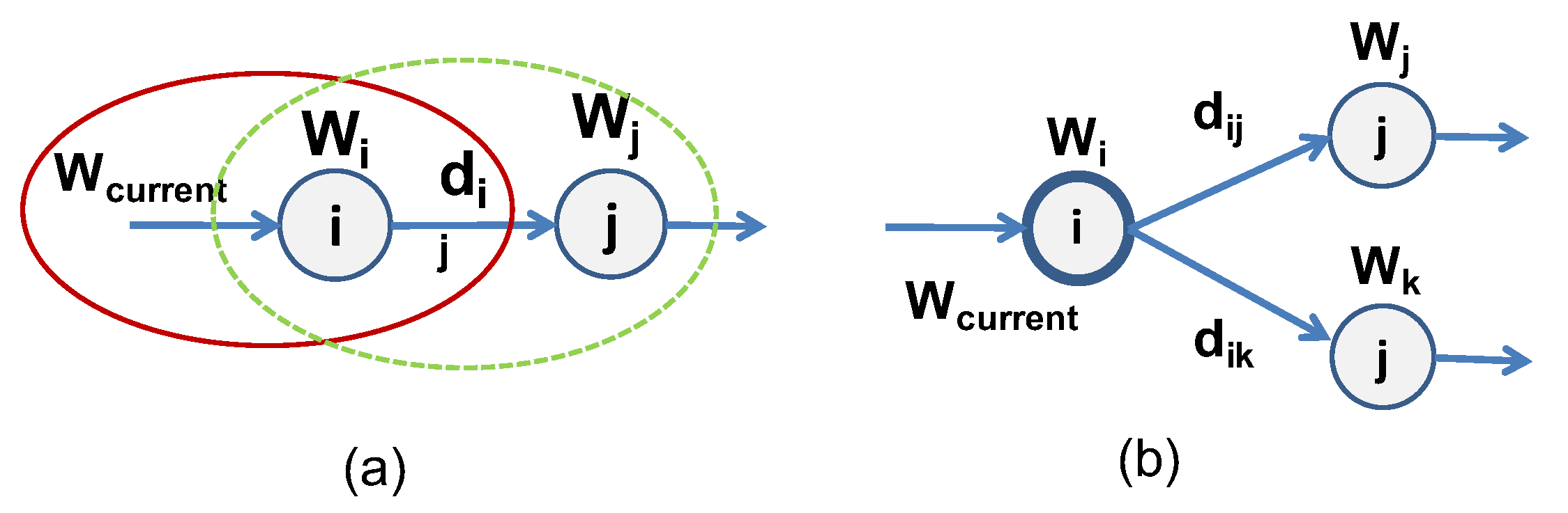$W_{current}$ is the current weight of the vehicle when reaching node i (Figure 5a); this metric, which we call Dx$W_r$ hereafter (i.e., distance times residual weight), uses the information contained in the solid oval circle.

Figure 5. Features of the Target Metric: Generic instance between two nodes i and j (a); and a greedy decision based on this metric (b).

By accruing this quantity over the delivery sequence, we would therefore be able to measure the area below the curves in the (weight, distance) space of Figure 1 as a proxy of the total energy spent.

Therefore, as the delivery problem is an instance of TSP, intuitively one could be tempted to run some TSP heuristic algorithm using the above cost in place of distance as in traditional TSP instances. Although approximate, (besides also neglecting battery non-idealities), this strategy will leverage well-consolidated heuristics for the solving the TSP and could be relatively efficient. Unfortunately, there is a subtlety in this argument. TSP formulations do assume the use of a “static” metric, i.e., whose value does not depend on the currently built solution, such as distance. As a matter of fact, state-of-the-art TSP heuristics rely on the calculation of the MST algorithm as a pre-processing. This is because the cost of a MST is the simplest lower bound for the TSP: it can be shown that the removal of one edge from any Hamiltonian cycle (i.e., a solution of the TSP) yields a spanning tree [11].

Algorithms to compute the MST systematically grow the tree by greedily picking edges in increasing order of the cost function, which clearly implies the need of a “static” metric, otherwise it would not be possible to guarantee global optimality by using local optimal choices (e.g., shortest edge) at each step. It is therefore immediately clear that the above cost function $d_{ij}\times (W_{current}-W_i)$ cannot be used in a conventional TSP algorithm and in particular based on MST, for two reasons. First, MST runs on an undirected graph and there is no intuition about in what direction the edge is traversed. Secondly, and most importantly, MST algorithms take a “local” greedy decision independent of the specific previous decisions; this is at the basis of greedy algorithms, in which the global optimum is a sequence of locally optimal choices. Therefore, even replacing the traditional distance-based metric in the MST with Dx$W_r$, it would simply not work, as shown in Figure 5b) (notice that for simplicity we assume the graph is directed to emphasize the direction of the delivery path).

Consider the decision to be taken at node i, at which we arrive with a given value of $W_{current}$. Without loss of generality, let us assume that there are only two possible choices at i, i.e., nodes j and k. A MST algorithm based on Dx$W_r$, since $W_{current}$ represents a “state” information of the current path at i and as such is a fixed value, will then greedily pick the edge with smallest value $min(d_{ij},d_{ik})$ to decide about whether to grow the MST along j or k. In other words, as $W_{current}$ does not change, $min((W_{current}-W_i)\ast d_{ij},(W_{current}-W_i)\ast d_{ik})$ and $min(d_{ij},d_{ik})$ result in the same choice.

Therefore, as already shown by the example of Section 2, the energy-optimal (or more precisely, Dx$W_r$-optimal) solution can only be obtained by enumeration of all the possible paths. A greedy, local metric used for a MST-based TSP algorithm would then result in strongly sub-optimal solutions even if we should adapt an MST algorithm to use Dx$W_r$.

Algorithms Used in Our Analysis

Based on the previous discussion, an exhaustive exploration of all paths to collect the one with the smallest cumulative Dx$W_r$ is the only way to achieve the optimal solution. This algorithm has obviously factorial complexity ($O(n!)$ for n vertices), which is clearly applicable only to small instances and can be used for evaluating the quality of different approximate algorithms.

Concerning TSP-based algorithms, the computational complexity of the TSP heuristic with the best approximation, i.e., Christofides’ algorithm, is $O\left(n^3\right)$, assuming that the graph is fully connected [11]. Although polynomial, cubic complexity can already be significant as the number of instances grow in the order to a few tens. Therefore, given the approximations of a TSP-based solution (the intrinsic approximation of the algorithm plus that of the metric described above), it makes sense to devise a simpler and greedy algorithm that builds up the cycle as a path, one edge at a time, starting from the depot, possibly using different greedy metrics. The greedy heuristic would clearly be linear in the number of nodes. Should some of the greedy heuristics be roughly as approximate as the TSP heuristic, it would at least guarantee that it can handle larger problem instances.

This choice would allow one to use the Dx$W_r$ metric that more closely tracks the energy value; by forming a path, in fact, we can calculate the equivalent of $W_{current}$ for the path being built. Moreover, since we start from the depot node, edges have an implicit direction and Dx$W_r$ can be calculated correctly. The approximation lies obviously in the fact that the greedy solution is not optimal, and, unlike the TSP heuristic, the approximation cannot be bounded. Christofides’ algorithm, for example, can be shown to yield a solution that is no more than 3/2 of the optimal cost.

In our analysis, we therefore compare three classes of algorithms to solve the optimal routing problem:

• a set of algorithms based on the exhaustive enumeration of all paths, which are applicable only to small instances and used to evaluate the quality of the approximations;
• heuristic greedy algorithms using different metrics;
• heuristic TSP algorithms using different metrics.

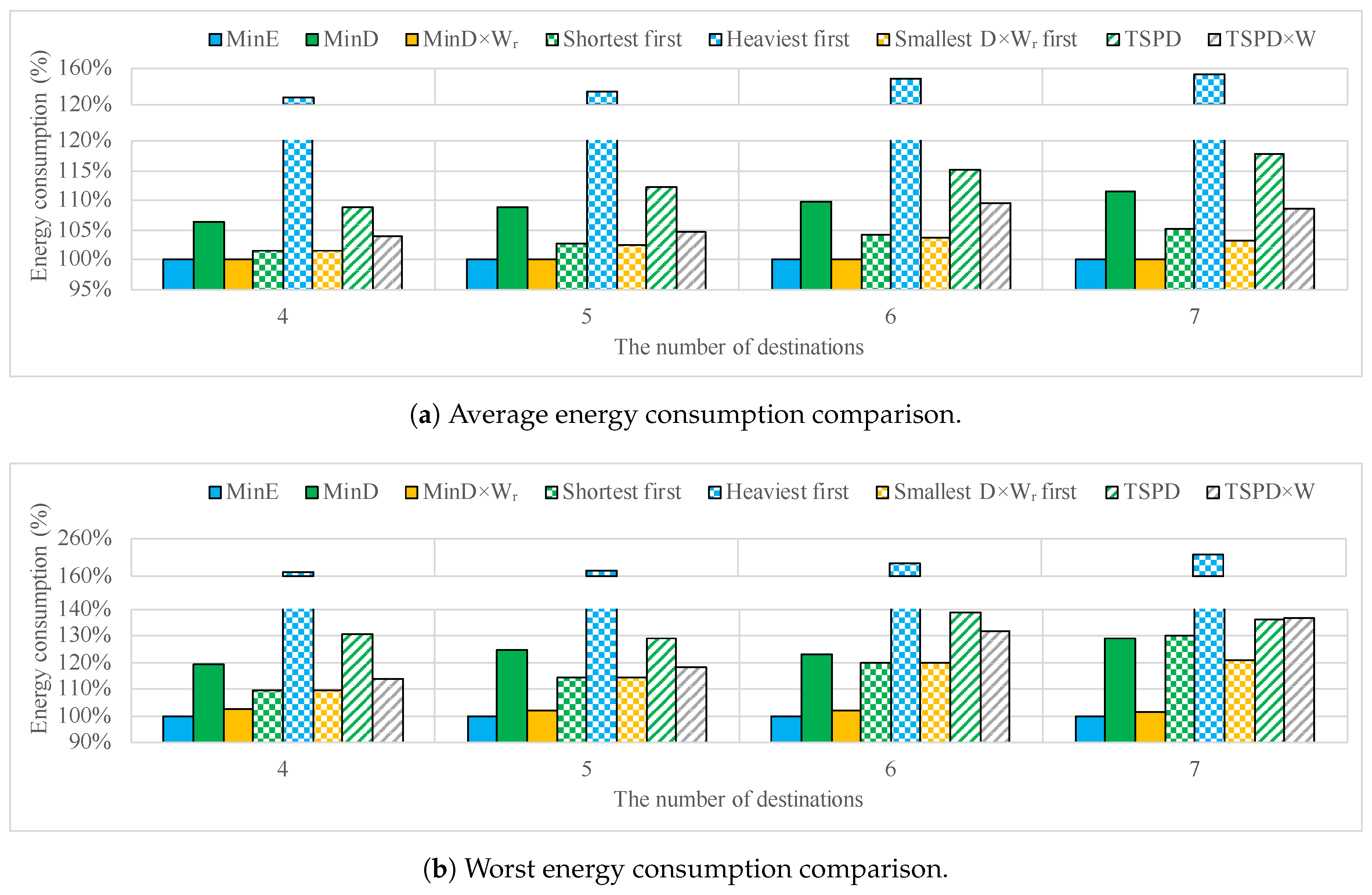
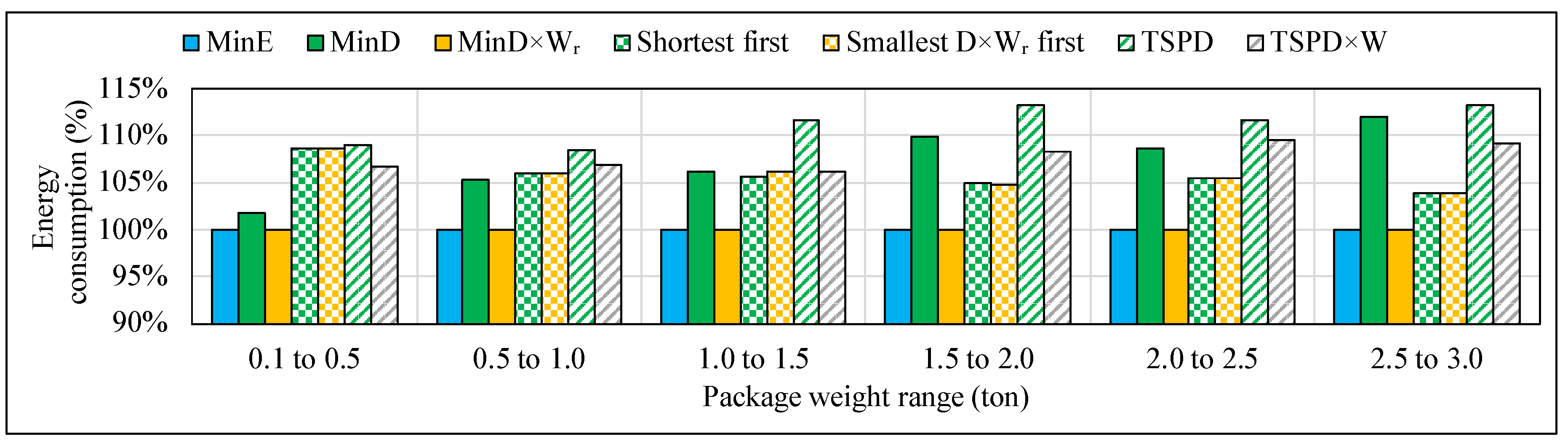
They are listed in Table 1 where algorithms belonging to the three above categories are separated by a double line in the table. Each algorithm is labeled with an abbreviation for ease of reference in the simulation results.

Table 1. Exhaustive exploration of paths: list of algorithms.

Name	Description
MinD	Paths are sorted in order of total length, and the shortest path is selected.
MinDx$W_r$	Paths are sorted in order of total $D\times W_r$ and the path with the smallest aggregate value is selected.
Heaviest first	Paths are built by greedily choosing vertices in decreasing order of weights.
Shortest first	Paths are built by greedily picking edges starting from the depot node in increasing order of distance.
Smallest Dx$W_r$ first	paths are built by picking edges starting from the depot node in increasing order of $D\times W_r$.
TSPD	TSP heuristic algorithm using distance as a metric.
TSPDxW	TSP heuristic algorithm using DxW as a metric.

The TSPDxW heuristic of the last line requires a further explanation. Given that, as shown above, using Dx$W_r$ in a TSP based algorithm would be immaterial as it will coincide with a distance-based metric, we devised an alternative metric that mimics Dx$W_r$ but that is suitable for a TSP-based heuristic. This metric, which we call DxW, assumes: (i) a 50% chance of traveling the edge in each direction; and (ii) approximates $W_{current}$ with the total weight (vehicle + payload). This results in a quantity that does not depend on the currently built solution, and uses also the information about the destination node (as shown in the dashed oval of Figure 5a), i.e.,

$$d_{ij}\times (W_{total}-(W_i+W_j)/2).$$

Notice that a plain “Shortest first” and “Smallest Dx$W_r$” would be the same algorithm. Therefore, to resolve this problem, for “Smallest Dx$W_r$ first” algorithm, we used $d_{ij}\ast (W_{current}-W_j)$, which considers both: (1) shortest distance first with $d_{ij}$; and (2) heaviest package first by abstracting weight of the destinations $W_j$ from $W_{current}$.

5. Simulation Results

5.1. Simulation Setup

5.1.1. Powertrain Model

We implemented a powertrain model of a Tesla Semi truck from the vehicle specification based on the presentation by Elon Musk; this is currently the only source of information for the specs as Tesla is preparing to release the Semi in 2020 or later [6,18]. The powertrain consists of four Model 3 electric motors; each motor is a three-phase AC permanent magnet electric motor with maximum power of 192 kW from 4700 to 9000 RPM, and maximum torque is 410 Nm below 4500 RPM [19,20]. We estimated curb weight of Semi as the sum of typical weight of class 8 truck and battery pack weight [21].

We first implemented a vehicle model in ADVISOR (ADvanced VehIcle SimulatOR) [22] by using the above vehicle specification. Then, we extracted the coefficients of EV powertrain model with a number of ADVISOR simulations, as described in [23]. Table 2 summarizes the model coefficients of Tesla Semi. We compared the results computed between the derived power model and ADVISOR to validate the model we used. Figure 6 shows the difference between the estimation of power consumption by the ADVISOR vehicle simulator and the powertrain models we derived; the normalized root-mean-square error is 4.93%.

Table 2. Powertrain model coefficients for Tesla Semi truck.

$\alpha$	0.098	$\beta$	10.1522	$\gamma$	1.006	$\delta$	2.5 × 10−5	$C_0$	10000
$C_1$	0.03	$C_2$	0.02598	$C_3$	1.54 × 10−5	$ϵ$	0.5912	$\zeta$	0.0

Figure 6. Powertrain model validation results compared with ADVISOR.

5.1.2. Battery Pack Model

There is no exact specification of battery pack in Tesla Semi truck until now; therefore, we assumed that each electric motor is connected to one battery pack of Model 3 in our experiments. Each battery pack is composed of four modules that are connected in series; each module consists of Panasonic NCR18650B 3400 mAh Lithium battery cells arranged in a 46p24s configuration [24].

Table 3 summarizes the physical electrical parameters of each cell, each module, and the whole battery pack.

Table 3. Electrical parameters of the battery pack.

Parameters	Cell	Module	Whole Pack
Nominal Capacity	3400 mAh	156.4 Ah	156.4 Ah
Nominal Voltage	3.6 V	86.4 V	345.6 V
Cut-off voltage	2.75 V	66.0 V	264.0 V

We built our battery single cell model based on the measurement data by adopting the method described in [9]. We assumed such 7104 battery cells in the pack to be ideally balanced in the following experiments, and then built battery pack model, as indicated in Section 3.2. Concerning the regenerative braking phase, we assumed that regenerative charging efficiency is 20% in our simulation, i.e., 20% of the kinetic energy is converted to electric energy and transferred into the battery pack.

5.1.3. Simulation Framework

We adopted the simulation framework proposed in [3], which targets the modeling and simulation of energy flow in the EV. The simulation framework is built by SystemC and SystemC-AMS, which are the extension of C/C++ with libraries to describe HW constructs and analog/mixed-signal subsystems. SystemC-AMS provides different abstraction levels to cover a wide variety of domains, three different Model of Computations (MoCs) supported by SystemC-AMS that allow the simulation framework to integrate circuit equivalent battery model and empirical powertrain model simultaneously. Another main advantage of the SystemC-AMS simulation framework is the fast simulation speed while keeping the same accuracy with regard to state-of-the-art tools such as Matlab/Simulink, with speedups up to two orders of magnitude and a high level of accuracy. Such quick estimation of energy consumption of EV and the battery lifetime give the opportunity to conduct exhaustive exploration in a short time for different delivery routes in our following experiments.

5.2. Simulation Results

5.2.1. Comparison Against Exact Results

In this section, we compare the energy consumption of various delivery strategies based on different policies for a set of small-sized (4–7) instances for which an exhaustive exploration of all the possible delivery paths is feasible.

For each number of destinations, we randomly generated 50 instances with different distributions of locations of the depot and of the destinations by uniformly distributing them in a 30 km × 30 km area. We selected the area for the delivery so that all the delivery sequences can be completed without exhausting the battery energy before returning to a depot. For each of the 50 instances, package weights for each destination were chosen as uniformly distributed from 0.1 to 3 ton.

For each problem instance (destination and weight distribution), we calculated by exhaustive exploration the route yielding the smallest value of energy for a number of metrics. Energy was calculated by conducting simulation described in Section 5.1. In this test example, a constant speed of 76 km/h was assumed, which was the average truck speed in metropolitan area interstates in the US in 2015.

Figure 7a shows the energy consumption of the optimal route, averaged over the 50 instances, for problems with 4–7 destinations and for the set of algorithms described in Table 1.

Figure 7. Energy consumption for different metrics (exhaustive exploration).

The leftmost blue bars represent the optimal routes yielding the minimum energy consumption among all routes, obtained by computing the actual energy consumption per each segment using the battery model. This is the reference value against which the other results were compared. All the other bars refer to solutions (i.e., routes) returned by the above algorithms and evaluated using the battery model. The objective of the simulation was to check how the greedy algorithms (TSP-based or not) differ from the optimal solution and how the error increases with increased problem sizes. Bars in the plot are in the same order as in Table 1. For ease of reading, bars referring to path-based algorithms (first part of the table) are shown as solid bars, whereas those referring to greedy or TSP algorithms are shown as patterned bars.

Concerning path-based algorithms, we can notice how the MinDx$W_r$ metric (third bar from left) tracks very well the true energy value, much better than distance alone (second bar from left). Concerning approximation algorithms, as a first general comment, we can see that all algorithms overestimate the actual energy consumption. Then, we immediately observe that weight alone (Heaviest-first) tracks quite poorly the actual consumed energy, somehow contradicting the intuition suggested by the battery property; the distance from the reference is already $>20$% even for the four-destination instance. Although the actual error may differ depending on the weight distribution (as shown in Figure 1), the results are the average 50 different runs, thus we can safely assume this is not a good metric. Notice also that the tracking error increases with larger instances.

Another observation is that a traditional TSP with distance metric (second bar from the right) performs reasonably only for the smallest instance; that average error increases quickly and is already around 18% for seven destinations. Therefore, we can also rule out this algorithm from the list.

The remaining ones (Smallest Dx$W_r$ first, Shortest first, and TSPDxW) have errors below 10%, with the greedy algorithms being below 5% and scaling better with problem size than TSPDxW. Especially, Smallest Dx$W_r$ first algorithm saves energy consumption from 6.58% to 12.46% compared with traditional TSPD algorithm. The gap between the best one and TSPD increases by the number of destinations.

Figure 7b shows the worst case error among the 50 instances for the same set of algorithms. Results are consistent with average error, with the maximum error being significantly larger than the average one. The greedy algorithms have show again the best results, in terms of both error and scalability. The Smallest Dx$W_r$ is the only algorithm with worst-case error around 20% (as opposed to about 30–35% of the others) for the seven-node case.

5.2.2. Comparison by Package Weight Distribution

In this section, we discuss how the error increases with the increased package weight. Figure 8 shows the energy consumption of different metrics by package weight distribution. Each column means different weight distribution of delivery package: 0.1–0.5, 0.5–1.0, 1.0–1.5, 1.5–2.0, and 2.5–3.0 ton, respectively. In this comparison, one depot and seven destinations were uniformly distributed in a 30 km × 30 km area, and we extracted average energy consumption of 50 instances by different metrics. In order not to provide unnecessary information, we do not consider MinDx$W_r$ and Heaviest first metrics here because these metrics show either sufficiently accurate or irrelevant results from the previous section.

Figure 8. Energy consumption by package weight distribution.

When the weight of the package is less than 0.5 ton, the sum of all package weight can be ignored in most instances compared with total weight of the electric truck. Thus, all results by different metrics show less than 10% error. As the range of the package weight increases, however, the effect of the package weight on the overall energy consumption increases. Therefore, metrics considering distance only show worse results, namely the exhaustive exploration with distance (minD) and the Traditional heuristic TSP (TSPD). On the other hand, heuristic TSP with DxW (TSPDxW) and two other greedy heuristics show less than 10% error for all weight ranges.

5.2.3. Application to Larger-Scale Instances

We generated a number of instances with 10, 20, 30, 50, and 100 destinations; for each problem size, we generated 20 random instances and collected the average value of energy and execution time. In all cases, weights were scaled so that the delivery task could be completed.

Figure 9 compares the absolute energy values for the three competitive algorithms resulting from the previous section: one TSP with the proposed metric (TSPDxW) and the the two greedy heuristics (Shortest first and Smallest Dx$W_r$ first). From the results in Figure 7a we know that all approximations are overestimations, thus we can assume that lower values of energy imply higher accuracy. In Figure 9, the Smallest Dx$W_r$ first shows the best results: its energy consumption is 10% smaller than the TSP heuristic and 4% smaller than the shortest first one, for the larger 100-node instance.

Figure 9. Greedy and approximate TSP algorithms on large problem instances.

Figure 10 shows the slowdown of the TSP heuristic with respect to the Smallest Dx$W_r$ first algorithm. The TSP execution time is obviously independent of the metric used (D vs. DxW). The TSP heuristic is significantly slower than the greedy method; the slowdown increases for increasing problem sizes, reaching 8.6 times for the 100 destination case.

Figure 10. Slowdown of TSP heuristics vs. greedy algorithm.

5.3. Case Study: Routing Problem in Real Roads

In the experiments presented in Section 5.2, the distribution of the locations were synthetically generated on a plane. In this section, we show the routing algorithms in a real case, consisting of a set of locations taken from a map and for which actual distances, road slope, and road traffic between destinations are taken into account. We generated 50 instances, in which package weights for each destination were chosen as uniformly distributed from 0.1 to 3 ton.

5.3.1. Extraction of Road and Elevation Information

We used Piedmont region in Italy as the delivery destinations. There are 10 destinations in Figure 11 including a depot. The destinations of the delivery are limited to towns or cities in the province.

Figure 11. Destinations for deliveries on real roads.

To travel between destinations, we cannot drive on a straight path, but we must use given roads. There are several route options connecting destinations to each other. Among them, the most recommended one by Google Maps is picked. We extracted the distance of each route and related average driving time.

Table 4 shows the altitude information of each city. We extracted average road slope from road distance and altitude difference between two cities. The average altitude difference among 10 cities is 84 m.

Table 4. Destination information.

City	Torino	Chivaso	Crescentino	Asti	Chieri
Altitude (m)	216	186	155	126	283
City	Alba	Bra	Carmagnola	Torino Airport	Rivoli
Altitude (m)	167	277	233	282	400

The practical distance of the route, road slope, and driving time are different by direction. Therefore, we implemented several matrices containing road distance, road slope, and driving time. The average distance of the roads is 44 km, and the average time for driving the roads is 51 min. The driving time was used to calculate average electric truck velocity. Therefore, the energy consumption for the delivery was obtained from the practical road distance, velocity, and road slope.

5.3.2. Simulation Results

Figure 12a shows the average energy consumption of the optimal route in the case study described in Figure 11 on the 50 instances with routing algorithms described in Table 1. When the number of destinations was four, we randomly picked one depot and four destinations among the 10 cities in Figure 11.

Figure 12. Energy consumption for different metrics (exhaustive exploration) on real roads.

Similar to Figure 7a, the leftmost blue bars (MinE) represent energy consumption by the energy-optimal routes among all routes. This is the reference value to compare with the other results. Bars in the plot are in the same order as in Table 1.

As confirmed by the results in Figure 7a, the path-based algorithms using the metric MinDx$W_r$ (third bar from the left) track very well the true energy value, much better than distance alone (second bar from left), in all simulation results with different number of destinations. Concerning approximation algorithms, weight alone (Heaviest-first) tracks quite poorly the actual consumed energy as in Section 5.2. The average error is up to 47.9%.

On the other hand, shortest first and Smallest Dx$W_r$ first metrics track the actual consumed energy very well. The average error is less than 10% for all numbers of destinations. Especially, Smallest Dx$W_r$ first shows the best results for all different number of destinations. A traditional TSP with a distance metric (second bar from the right) tracks well only for the smallest instance as in Figure 7a; average error increases up to 15.0%. TSP with a metric DxW shows better results than distance metric.

Figure 12b shows the worst case error among the 50 instances for the same set of algorithms in Figure 12a. The results are consistent with average error, but significantly larger. The best algorithms in Figure 12a (Smallest Dx$W_r$ first, Shortest first, and TSPDxW) again show the best results, in terms of both error and scalability. TSPD and TSPDxW methods are not better in some cases (e.g., six destinations) because triangular inequality is not applicable, and the distance between cities is asymmetric.

6. Conclusions

The total energy consumption for parcel delivery with an electric truck strongly depends on the order of delivery because battery efficiency is affected by how the transported weight changes over time. However, it is impossible to consider the transported weight changes with the traditional routing algorithms, which use “static” metrics such as distance. In this paper, we demonstrate that the functions of weight and distance as metrics provide significant energy reductions with respect to the traditional routing algorithms. A traditional TSP with distance metric performs reasonably only for the smallest instance; average error increases quickly. On the other hand, a greedy algorithm minimizing driving distance by residual weight (Dx$W_r$) shows better results with almost 10× faster runtime. We also performed a comparison in the real delivery case, where curved and sloped roads connect cities. In this case study, the greedy algorithm also shows better results than traditional TSP. In addition, the package weight affects the result of routing algorithm. As we increase the package weight distribution, the gain by the proposed method increases.