1. Introduction
Artificial Ground Freezing (AGF) is a consolidation technique adopted in geotechnical engineering, when underground excavations must be executed in granular soils, or below the groundwater level [
1,
2]. The realization of relevant underground structures in urban areas often involves the management of constructive problems related to avoiding the presence of water in the excavation, especially if the soil has poor geo-mechanical proprieties. The artificial ground freezing technique has been extensively used in the last decades as an effective and powerful construction method, which provides ground support, groundwater control, and structural underpinning during construction. However, the use of this technology requires a good knowledge of frozen soil behavior and a robust numerical model able to predict ground movements around the excavation. This is important, especially in densely urbanized areas, where frost action is detrimental for surrounding structures.
The AGF method consists of letting a refrigerant circulate inside probes located along the perimeter of the excavation, at a temperature significantly lower than the surrounding soil. The water in the soil goes from liquid to solid phase, and it forms a block of frozen ground in the area surrounding the probes.
The process is, in general, divided into two different phases: a first “freezing phase”, that ends when the soil achieves the design temperature needed to start the excavation, and a “maintenance phase”, which is characterized by heat absorption in order to keep the temperature constant during the excavation [
3].
The main advantages of this technique, among the available ground consolidation and waterproofing technologies, are: (i) security and compatibility with the environment, since there is no injection, and the dispersion of products in the ground. Water already present in the ground is, in fact, frozen, using refrigerant fluids that are never directly in contact with the ground and groundwater, avoiding contamination phenomena; (ii) applicability to any type of soil, from coarse to fine grain and rocks [
3,
4].
Depending on the working fluid used, two types of methods can be identified: (i) the direct method, which is based on the use of liquid nitrogen entering the probes at a temperature of −196 °C and released in the atmosphere in gaseous phase at a temperature between −80 °C and −170 °C; (ii) the indirect method, which is based on the use of a mixture of water and calcium chloride (known as brine), whose circulation temperature can vary between −25 °C and −40 °C. A combination of the two previous methods is known as a mixed-method, which uses the direct method for the freezing phase, and the indirect method for the maintenance phase.
Several numerical and experimental works analyzing the AGF technique are available in the literature. Colombo [
5] in the first part of his work invokes a well-known approximate approach for the a priori evaluation of the parameters influencing the technique, such as the time required to reach the target temperatures, or the heat flow rate needed by the plant. The results proposed by the author, applied to Neapolitan tuff, were compared with those obtained from a series of numerical analyses conducted by using the finite element method as a discretization technique, and with experimental data measured on site during freezing operations carried out for the realization of the galleries for the stations of Piazza Dante and Piazza Garibaldi of metro Line 1 in Napoli (Italy). Papakonstantinou et al. [
6] first analyzed the experimental data of monitored temperatures in the ground during the freezing process, and then performed a numerical analysis through the FREEZE calculation code, a thermohydraulic software developed at the ETH in Zurich. The authors found that the thermal conductivity of the soil is an important parameter to be taken into account, and can be reasonably estimated by a posterior numerical analysis, if it not known a priori. Subsequently, Pimental et al. [
7] analyzed the results of three applications of the AGF technique in urban underground construction projects, comparing the experimental data with the thermohydraulic coupled code model FREEZE. The first case study concerned the construction of a tunnel for the underground in Fürth (Germany) in soft ground with significant infiltration flow. The second case study concerned a platform tunnel in a metro station in Naples, and aimed at the determination of relevant thermal parameters through retrospective analysis, and to compare the results obtained by using the forecasting model with on-site measures. In the third case, regarding a tunnel under the river Limmat in Zurich, numerical simulations were used to identify potential problems caused by geometrical irregularities in the well layout, in combination with infiltration flow. Russo et al. [
1] analyzed the experimental data collected during the execution of the excavation with the AGF technique, and developed a numerical model to evaluate stress in the ground during the freezing and defrosting of a frozen wall. The focus of the work was the settlement caused by the tunnel excavation, and the use of the AGF technique to allow the safe digging of a service gallery located half in the silty sand layer, and a half in the yellow tuff layer, below groundwater. The phases of the tunnel construction were accompanied by the monitoring of the measurements and control activities of the effects of the gallery excavation. The measurements collected during the construction process, in fact, allowed us to monitor the freezing-thawing process, and the change in volume related to the excavation, providing useful information for the future implementation of similar projects. Finally, the analysis in the test procedure was conducted using a complete three-dimensional (3D) model implemented in the DFM Flac3D package.
Vitel et al. [
8] developed a numerical model considering both the freezing tube and the surrounding ground. The model is based upon the following principles: (i) heat conduction around the well is solved by considering vertical heat transfer processes negligible compared to the trans-horizontal heat transfer; (ii) heat transfer in the freezing probe is reduced to a one-dimensional (1D) calculation. In this study, convection in the ground was not taken into account with respect to the heat conduction, and therefore, the effects of groundwater flow were not considered. Vitel et al. [
9] developed a numerical thermohydraulic model in order to simulate artificial ground freezing by considering a saturated and nondeformable porous medium under groundwater flow conditions. Marwan et al. [
10] presented a thermohydraulic finite element model integrated into an optimization algorithm, using the Ant Colony Optimization (ACO). This technique allowed researchers to optimize the positions of the freezing probes with respect to the groundwater flow. Kang et al. [
11] combined a freezing method and a New Tubular Roof (NTR) simulated by thermomechanical coupling analysis. The temperature range obtained in the freezing process indicated that the thickness of the frozen wall grows of about 2.0 m after 50 days of freezing. Moreover, the stability of the surrounding ground and the support structures in the bench cutting phase were also studied. Panteleev et al. [
12] focused on the development of a monitoring system for the artificial ground freezing process for a vertical shaft. The temperature in the wells was measured by using the fiber optic system Silixa, based on the Raman effect. Alzoubi et al. [
13] have evaluated the development of a frozen wall between two freezing probes, with and without the presence of groundwater infiltration for 2D geometry, by was using ANSYS. Fan et al. [
14] show a case study concerning the monitoring of frozen wall formation during soil freezing using brine, then developed a three-dimensional numerical model to analyze the temperature distribution. The numerical simulation was conducted by using ADINA software.
Based on the analysis of the available literature, the interest of the research community on the AGF technique is evident. Both experimental and numerical works can be found, however, more research effort is needed to numerically analyze the evolution of the process for real cases, considering the geometry of civil works and the development of the freezing probes in the ground. For these reasons, the authors have developed an efficient transient numerical model to effectively analyze heat transfer in the soil, and at the same time, save computing resources. The proposed approach is based on the coupling of a heat transfer model between the freezing probes and the surrounding ground with a heat transfer and phase change model of the soil, and for the first time in the literature, all of the phases of AGF process have been reproduced. The model was used as a preliminary predictive analysis for the construction of two tunnels in Napoli. The model has been validated against the data of Colombo [
5]. After validation, the numerical model has been employed to analyze a real case study of two tunnels between Line 1 and Line 6 of the metro station in Piazza Municipio, Napoli, southern Italy. The purpose of the work is to study in detail the heat transfer process during ground freezing for the realization of the tunnels. The analysis is carried out by employing a FEM-based model, using Comsol Multiphysics commercial software, to model artificial ground freezing during the whole processe.
The model developed in the present work allows us to simulate, for the first time in the literature, a mixed-method used for the freezing process, from the first phase based on nitrogen feeding, a maintenance phase, and a third phase that involves the use of brine. The maintenance phase is necessary to avoid the freezing of brine in the probes. The novelty introduced by this work relies on the development of a thermal analysis of the entire artificial ground freezing process, considering all the phases and the influence of the process on the thermodynamic behavior of a second nearby tunnel that was also subject to the AGF. Moreover, the excavation phase has been reproduced, by imposing a convective heat transfer condition related to the presence of men and machines, while the second tunnel was subject to AGF with a mixed method.
This paper is structured as follows: in
Section 2, the characteristics of the AGF technique are described, while in
Section 3 the numerical model developed is presented.
Section 4 reports the validation carried out against literature data. The results of the parametric analysis performed after model validation are reported in
Section 5, while conclusions are drawn in
Section 6 of the paper.
2. Description of AGF Technique and Case Study
Artificial Ground Freezing (AGF) consists of freezing the ground by means of heat transfer, with a refrigerant fluid circulating inside probes located along the perimeter of the excavation to be realized. In this way, the water contained in the soil undergoes a phase transition from liquid to solid, forming a block of frozen ground called a “frozen wall” in the area surrounding the probes.
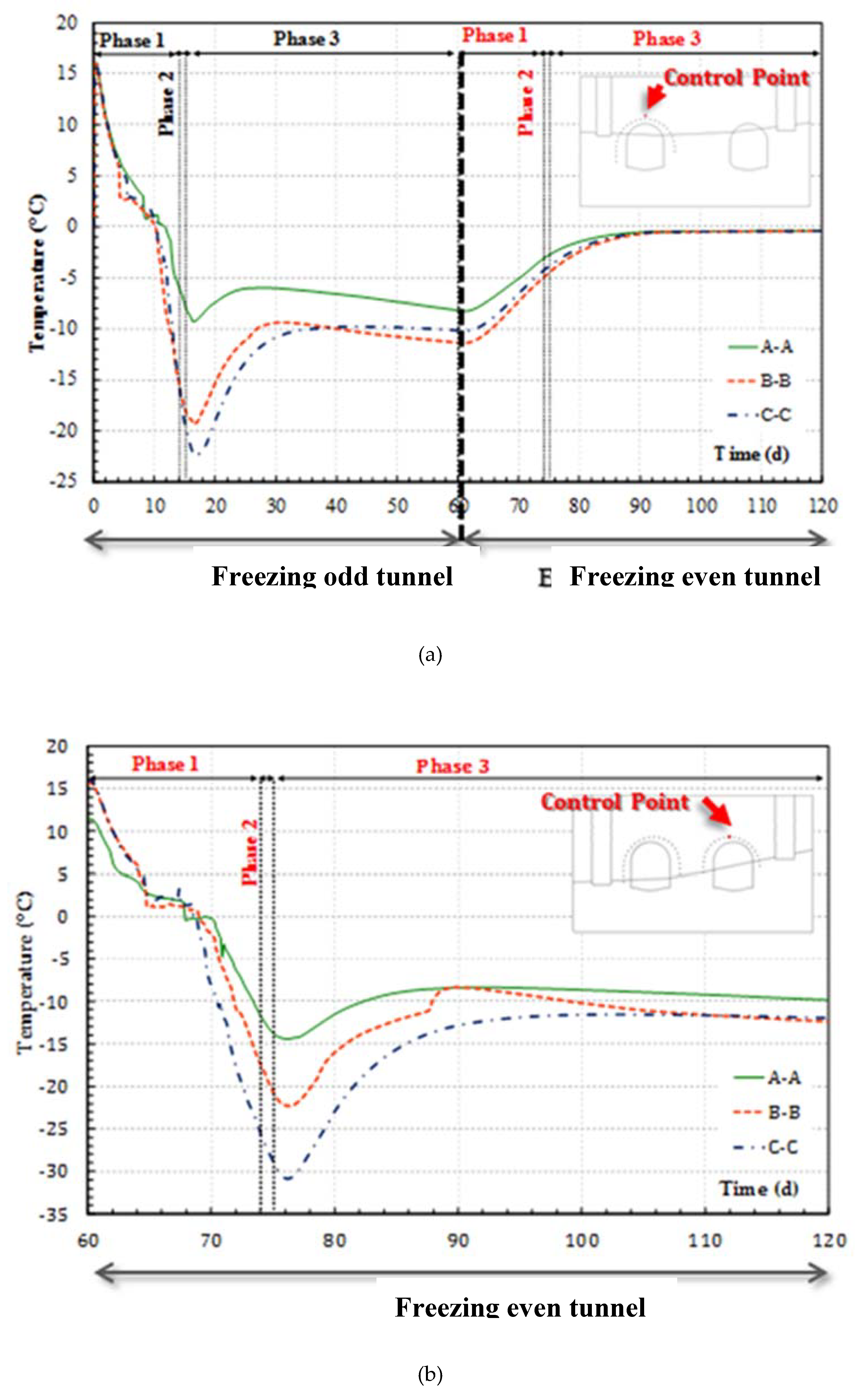
The mixed-method AGF process used for the Piazza Municipio galleries can be divided into different phases:
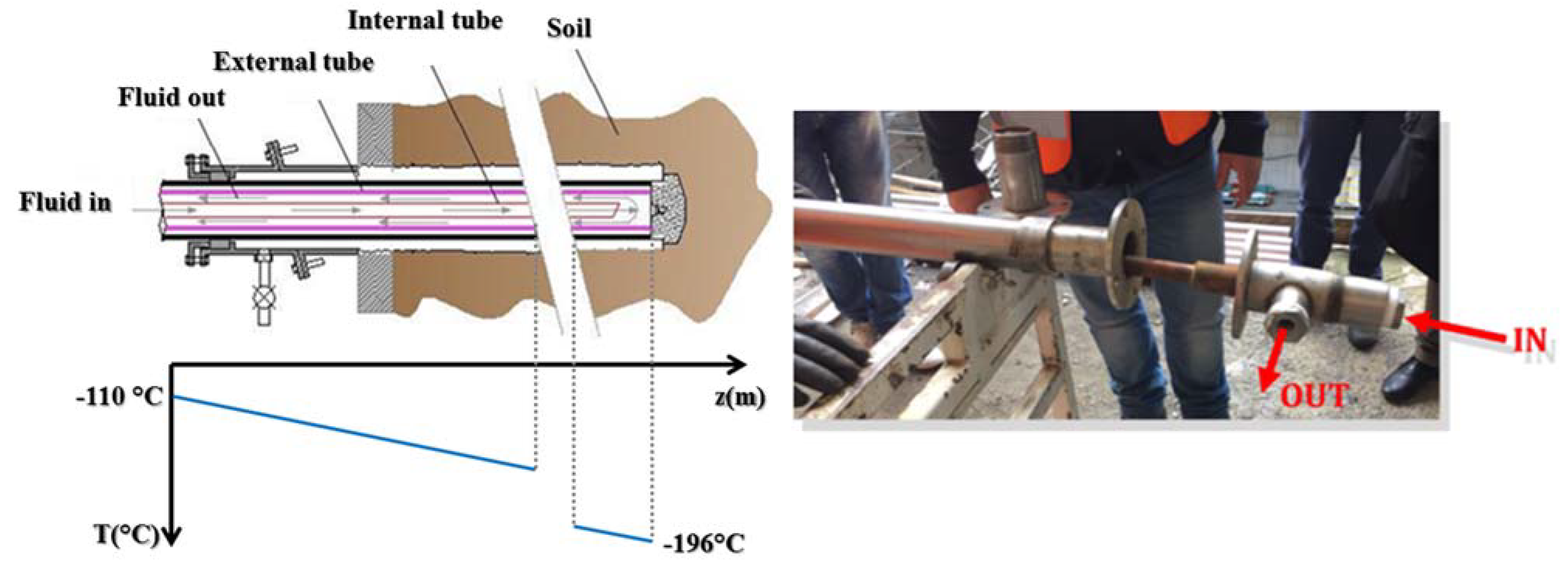
Phase 1-Nitrogen: The probes are fed with nitrogen at an inlet temperature of about −196 °C, while the expected outlet temperature is around −110 °C. The duration of Phase 1 is related to the time required for the formation of the minimum thickness of the frozen wall (1.5 m);
Phase 2-Waiting: At the end of nitrogen feeding, in order to obtain a temperature adequate for brine feeding, and to avoid brine freezing inside the probes;
Phase 3-Brine: Maintaining the ice thickness on the tunnel vault by feeding the probes with brine, at a temperature of about −35 °C. Phase 3 is used during the tunnel excavation, in order to maintain the soil temperature below water freezing over time, and the desired thickness of the frozen wall.
For the realization of two tunnels between Line 1 and Line 6 of the underground station in Piazza Municipio in Napoli, the AGF technique with the mixed method has been used. The choice to use this method is due to the possibility of combining the cryogenic power of nitrogen with the flexibility and safety of freezing with brine. It consists essentially of making complementary direct and indirect methods, using the same freezing probes.
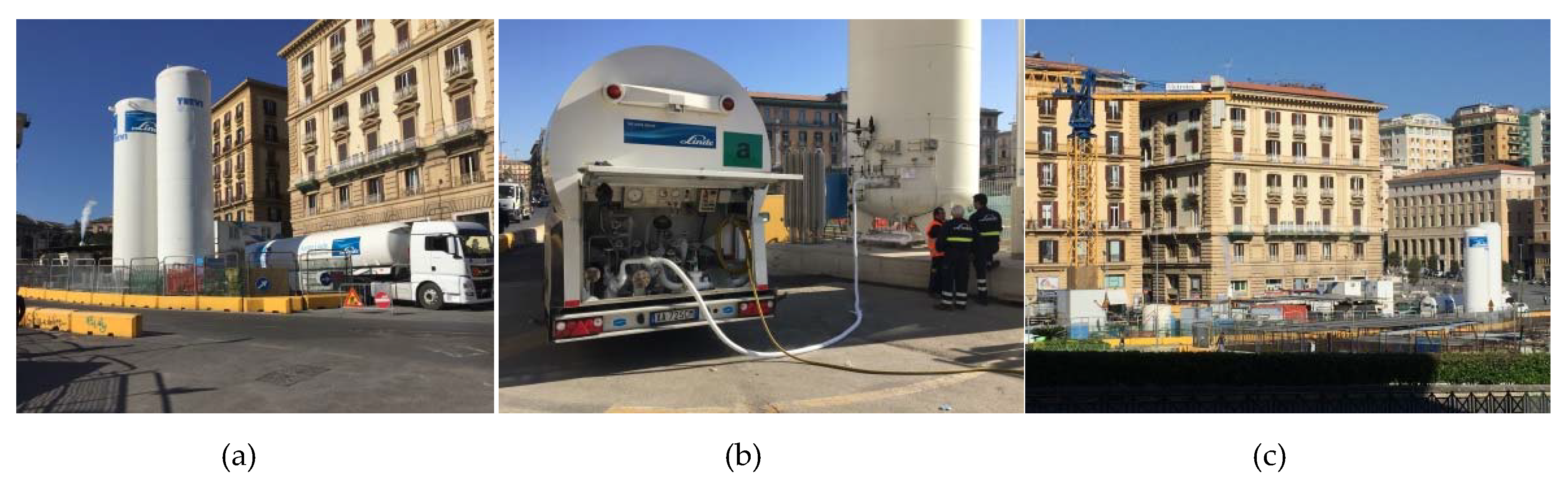
An overview of the nitrogen feeding procedure and system used is reported in
Figure 1, which reports the truck and tanks at the construction yard, and the loading phase of liquid nitrogen into the tanks.
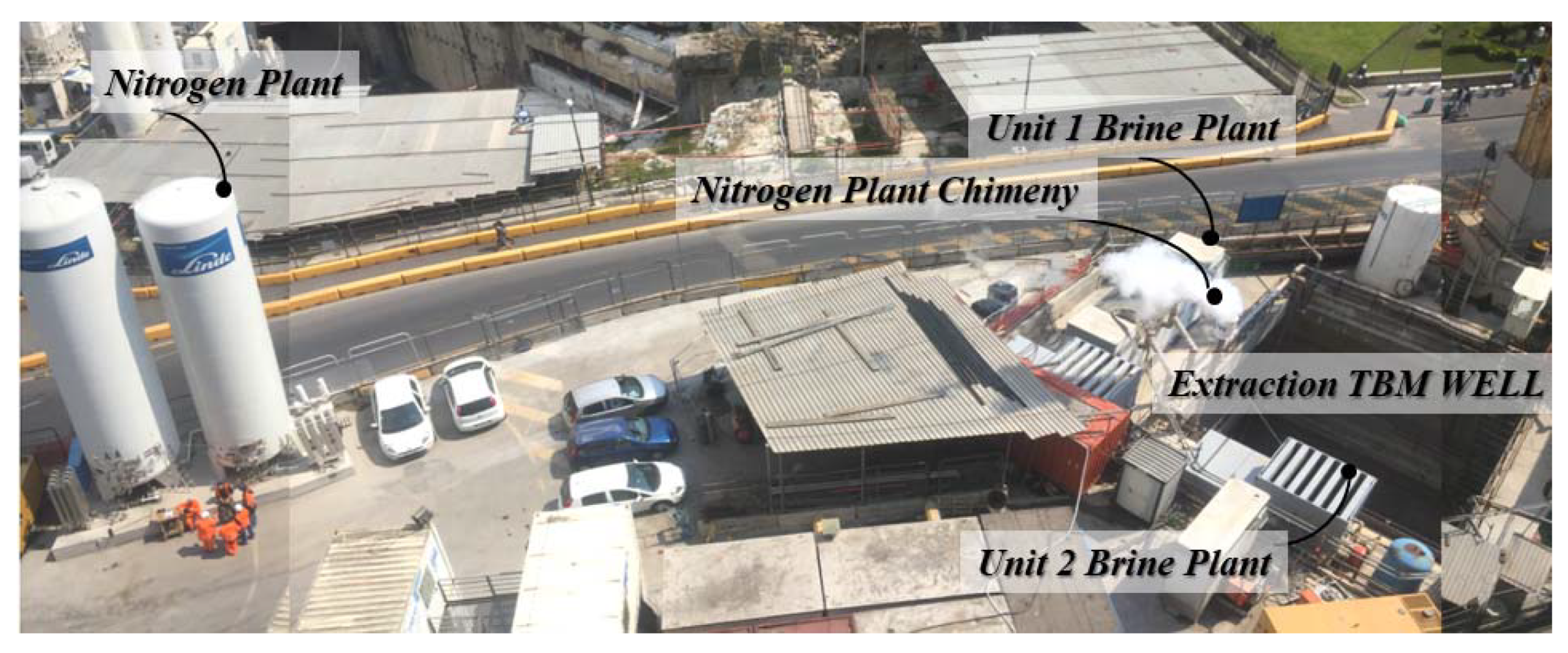
Figure 2 shows an overview of the construction site, where it is possible to see the nitrogen plant and the two brine refrigeration units. The nitrogen feeding system works by gravity. The brine is refrigerated by one unit, while the second is used as back up in case of the failure of the first one.
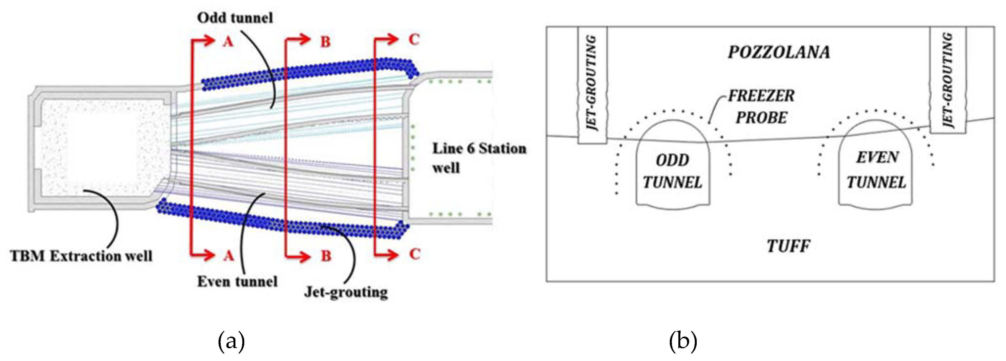
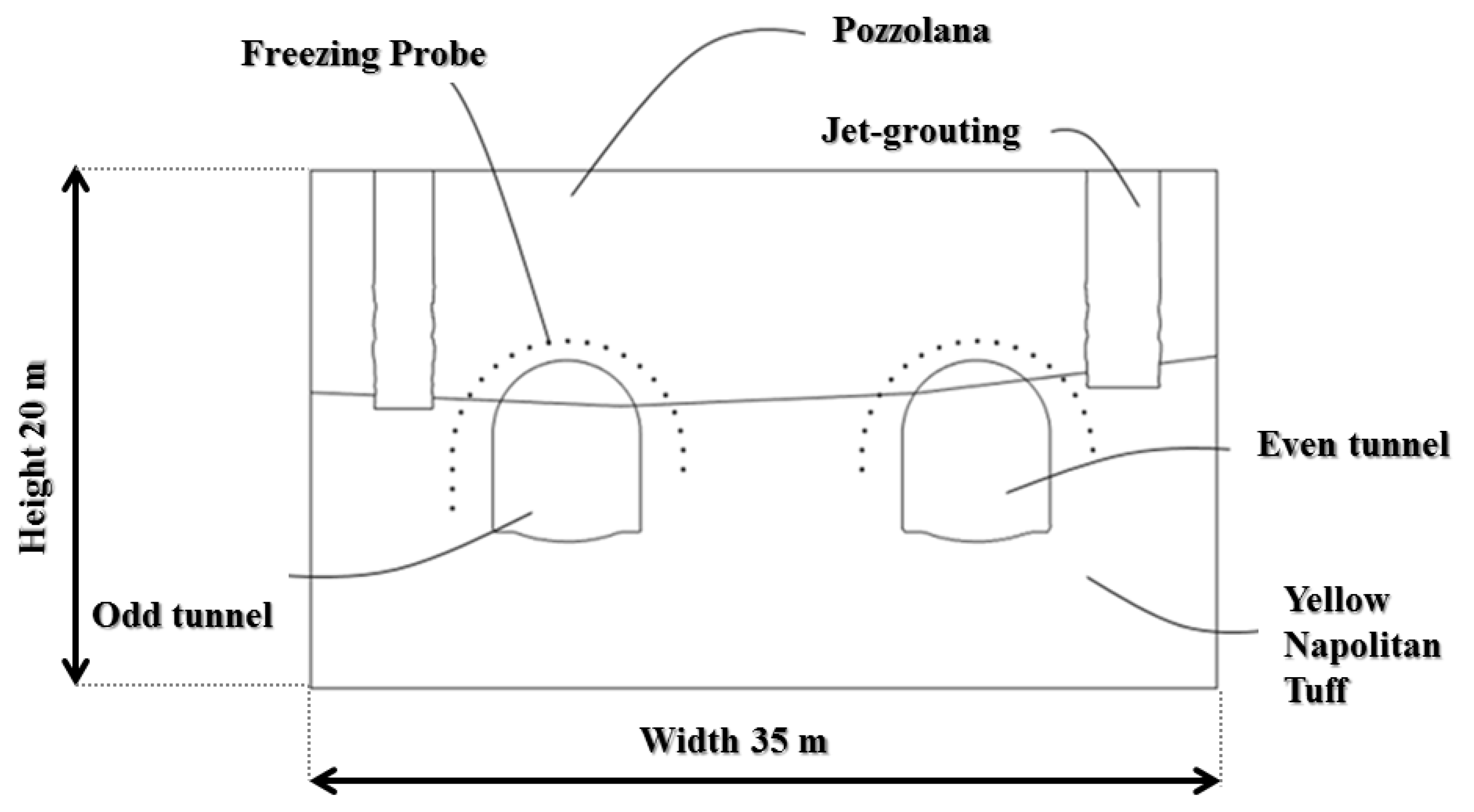
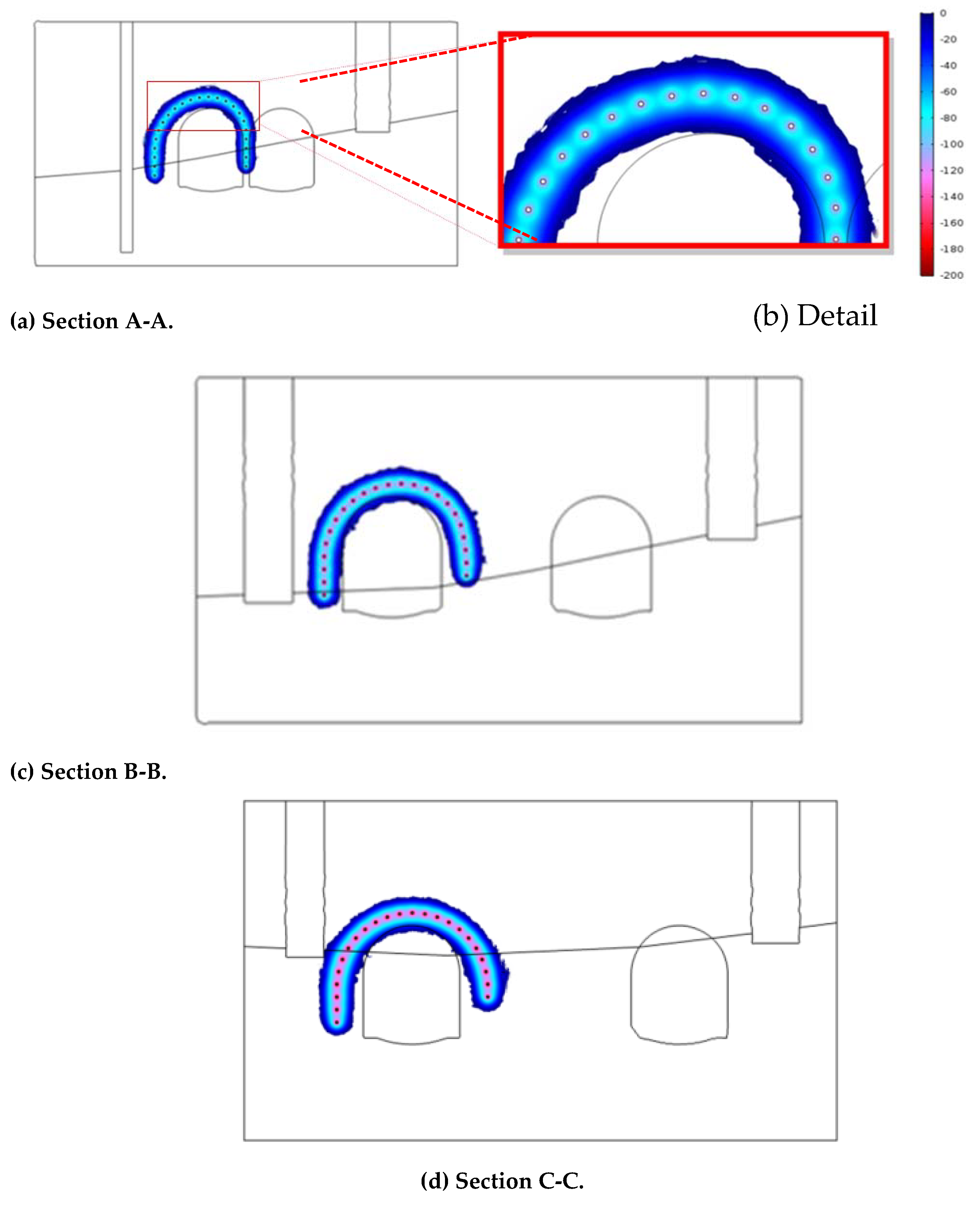
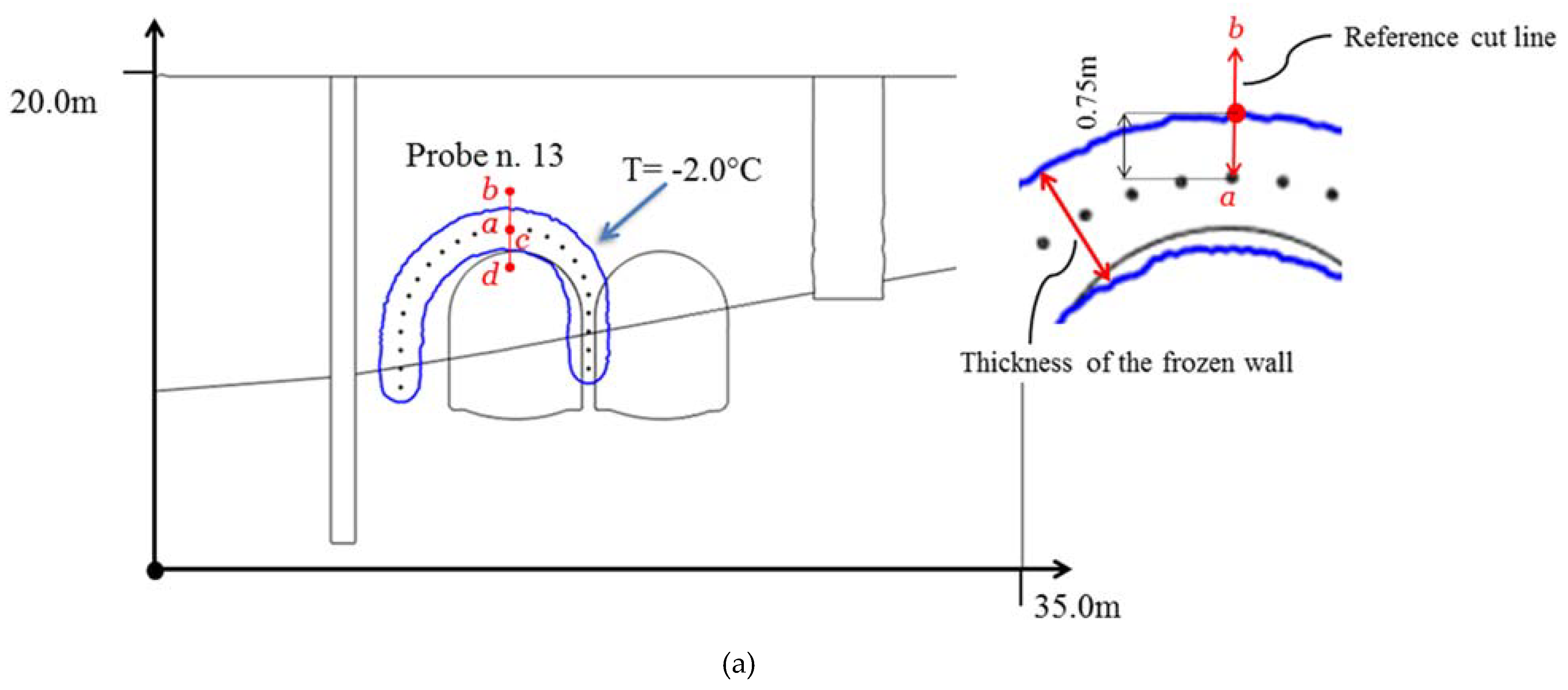
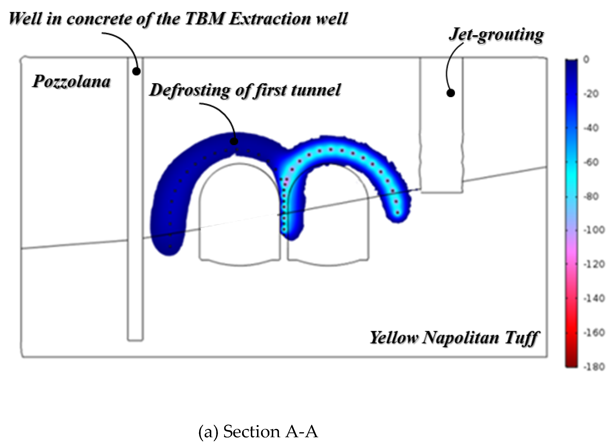
The present case study involves the construction of two tunnels for the connection between Line 1 and Line 6 of the Metro station of Piazza Municipio in Napoli, southern Italy. The soil affected by the excavation consists of a layer of pozzolana overlaying a bench of tuff. As shown in
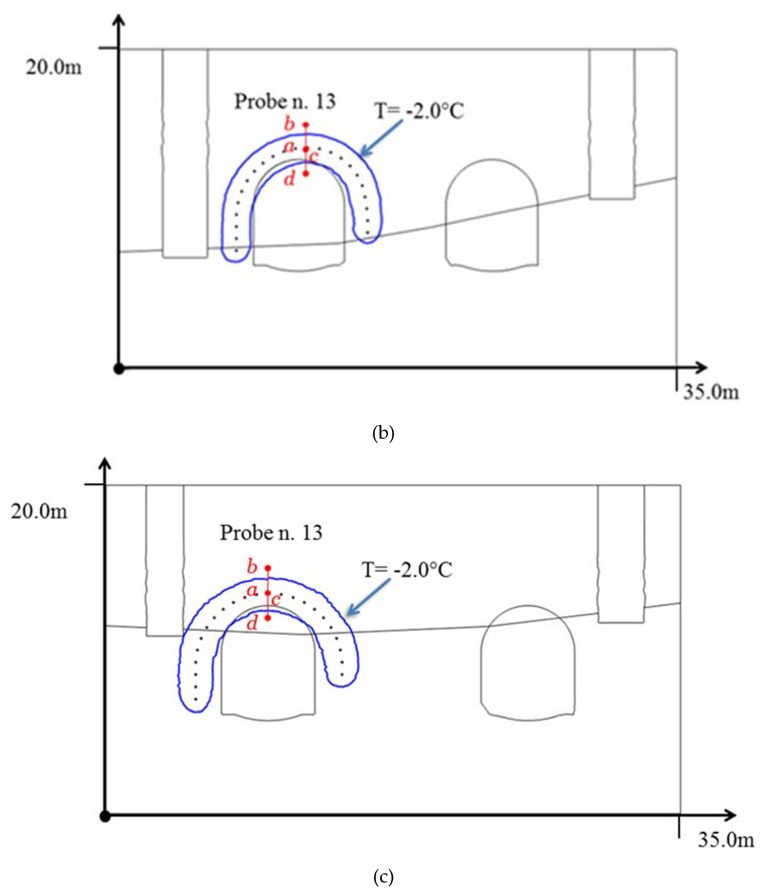
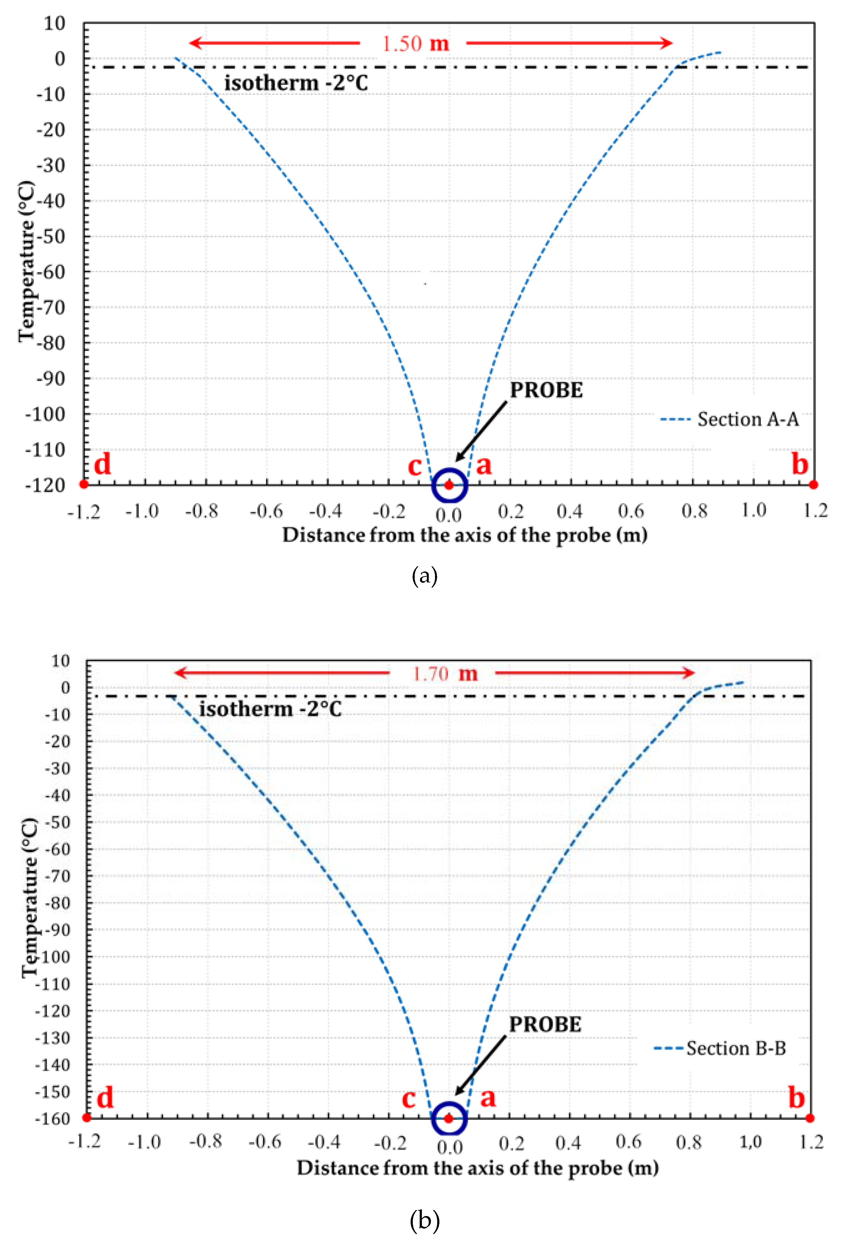
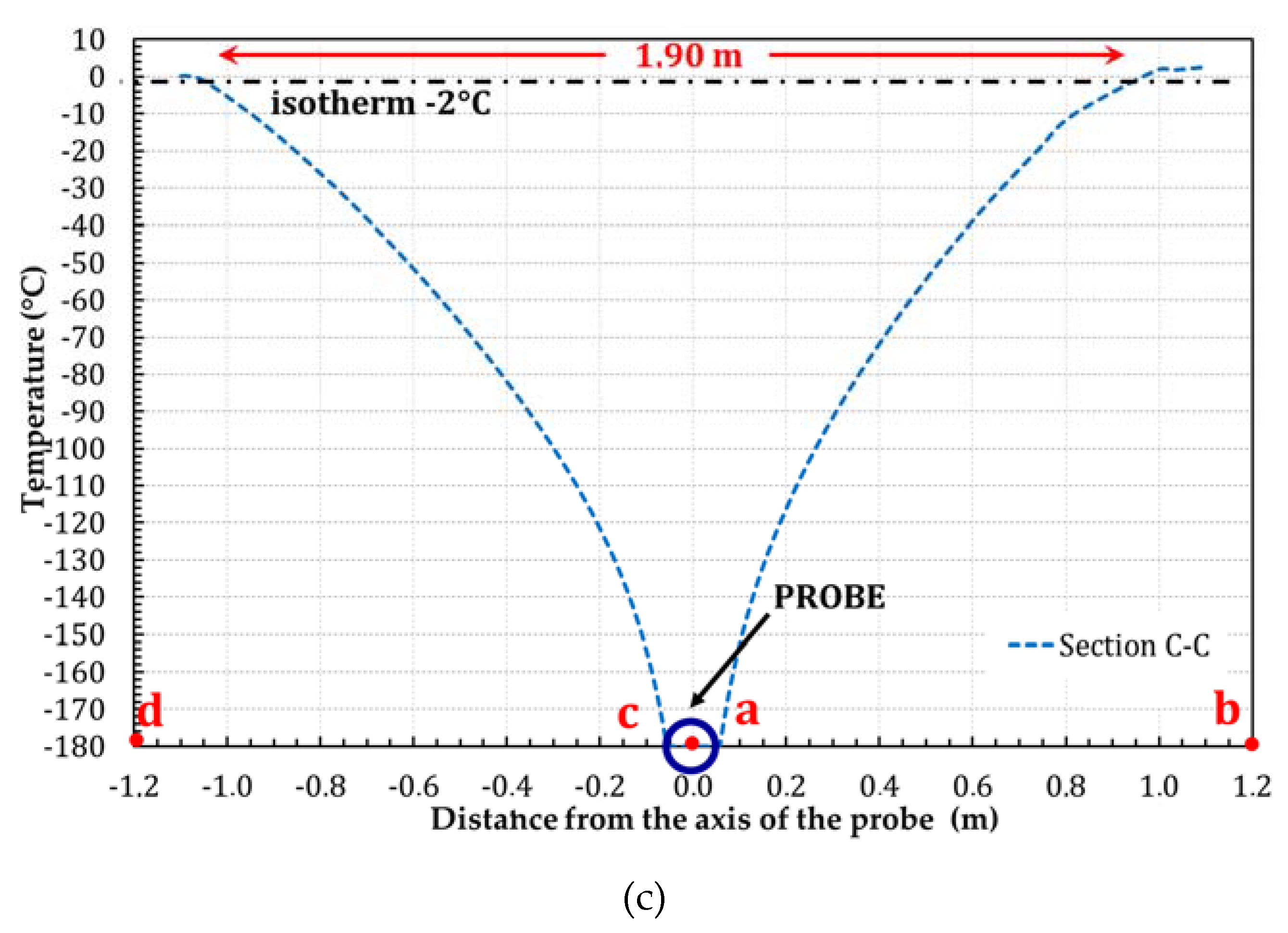
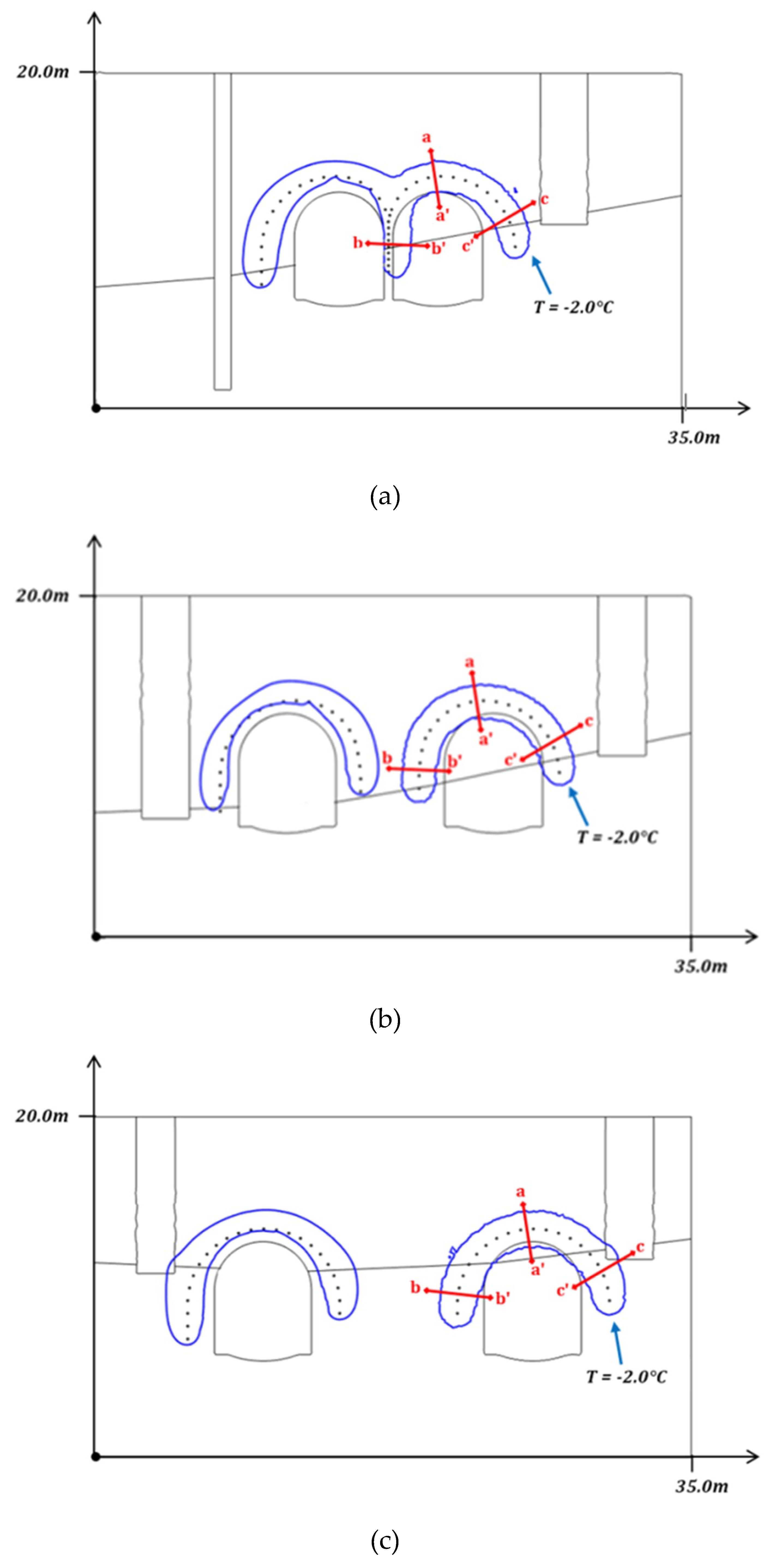
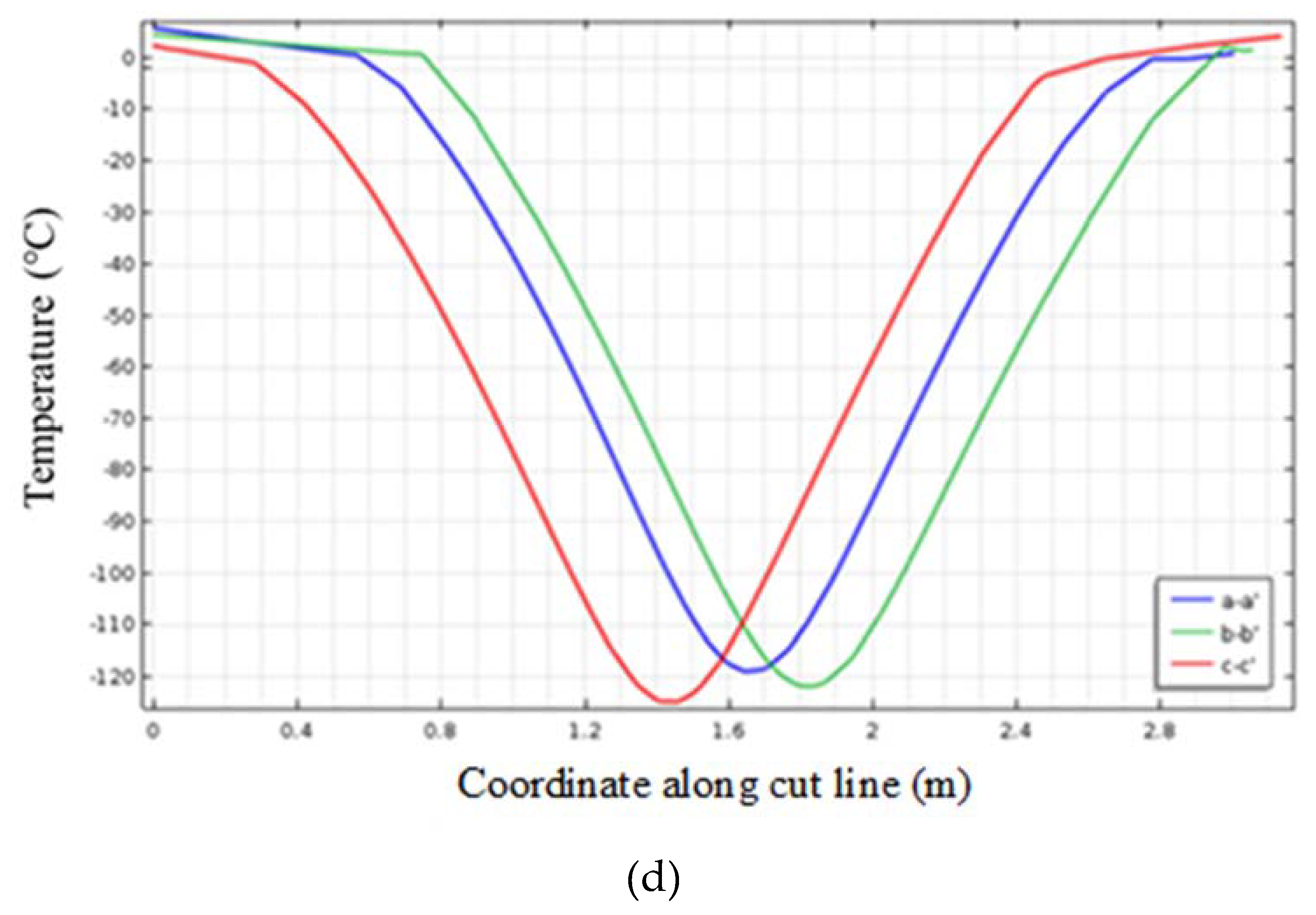
Figure 3a, the horizontal distribution of the freezing probes is influenced by the actual development of the two tunnels, that have a slight curvature. Instead, the freezing probes, for technological reasons, have a straight distribution along their axis. Section A-A is located at 5.0 m from the Tunnel Boring Machine (TBM) extraction well, section B-B is in a central position with respect to the tunnels, and section C-C is located at 5.0 m from Line 6 Station well.
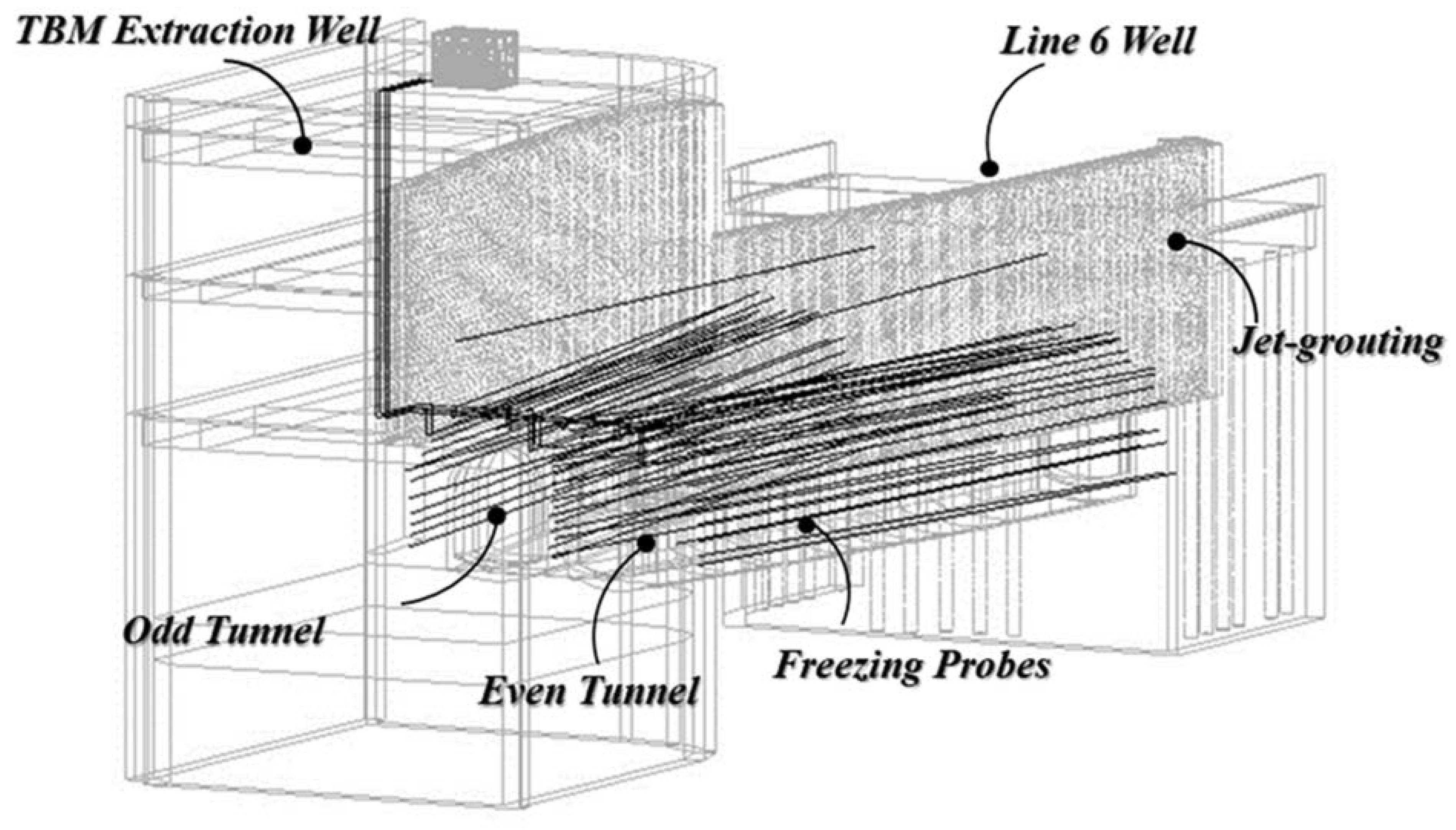
Figure 3b shows a cross section of the case study with the position of the freezing probes, while
Figure 4 shows the axonometry of the two tunnels connecting Line 1 and Line 6.
In order to construct the two tunnels connecting Line 1 and Line 6, the excavation of the odd tunnel occurred before the one in the even tunnel. The odd tunnel excavation began after freezing the soil around it, by cutting the diaphragm of the Line 6 station well (see
Figure 3), at the opposite point of nitrogen input into the probes, and continuing with the excavation one meter at the time, with the laying of steel ribs and spritz beton until the TBM extraction well was reached. Once the odd tunnel excavation operations were completed, the even tunnel was frozen and constructed.
On the exterior side of the tunnels, two jet grouting walls reaching the depth of the tuff bench had been employed with the purpose of containing fluids motion in the ground. The freezing of the tunnels has been realized using 43 freezing probes (23 for the odd tunnel, and 20 for the even one) with a length of about 40 m, arranged in an arch outside the excavation section with a constant wheelbase equal to 0.75 m. The installed probes are made up of two concentric tubes, as shown in
Figure 5. The outer one is made of steel and has a diameter equal to 76 mm, while the inner one is made of copper, with a diameter of 28 mm.
3. Mathematical Model of the Freezing Process
The model is based on 2D conductive heat transfer in the ground surrounding the probes, and takes into account the phase change phenomenon of water. The mathematical model has been implemented within the commercial software Comsol Multiphysics, based on finite element discretization technique, and has been solved by using the MUltifrontal Massively Parallel sparse direct Solver. The ground subdomain has a depth of 20 m and a length of 35 m, and can be considered sufficiently large to avoid thermal interference with the external environment, and sufficiently deep to assume an undisturbed soil temperature.
Figure 6 shows the cross section of the computational domain considered in the present analysis.
The assumptions underlying the present model are the following: (i) homogeneous and isotropic materials in each layer of the computational domain; (ii) thermophysical properties of the soil varying with temperature, between the frozen and unfrozen phases; (iii) for the whole volume of soil, phase transition takes place at a temperature of 0 °C within an interval of 1 °C; (iv) the temperature of the cooling fluid in the probes varies linearly along the axis; (v) heat transfer is purely conductive in the soil, due to the limited convective motion of the water in the ground.
3.1. Governing Equations
The problem under investigation has been simulated by means of a dynamic model reproducing the 2D conductive heat transfer in the ground [
15,
16], taking into account the phase change of water in the soil. The governing equation for heat transfer is reported as follows:
Transient conduction heat transfer
where
ρi is the density of the materials constituting the subdomain (kg/m
3),
cpi is the specific heat capacity (J/kg·K),
ki is the thermal conductivity (W/m·K),
T is the temperature (K), and finally,
Q is the heat generated or absorbed per unit of volume (W/m
3). This last term on the right-hand side allows us to model the latent heat of solidification, such as the heat absorbed or released at a constant temperature during the phase change of water in the soil. In fact, this phenomenon is characterized by a significant variation of the thermal diffusion coefficient and the specific heat of the saturated soil, in addition to the absorption of melting latent heat. The time-step employed in the simulations is equal to twelve hours.
3.2. Phase Change in the Soil
The formulation used in the present work provides the latent heat as an additional term in the heat capacity.
Instead of adding the latent heat L in the energy balance equation exactly when the material reaches its phase change temperature, Tpc, it is assumed that the transformation occurs in a temperature interval between Tpc − ΔT/2 and Tpc + ΔT/2. ΔT is the temperature interval which occurs within the phase change of water. In this interval, the material phase is modeled by a smooth function,
, representing the fraction of phase change during transition, which is equal to 1 below Tpc − ΔT/ 2 and to 0 above Tpc + ΔT ⁄ 2. The density,
, and the specific enthalpy, h, of the ground are then calculated as:
where
and
indicate the characteristics of the material during the different phases of water within the soil. The specific heat at constant pressure can be defined as:
that becomes, with the product derivatives:
where
and
are, respectively, equal to
and
. The term
is defined as:
and it is assumed equal to −1/2, before the phase change process, and 1/2 at the end of the process.
Therefore, the specific heat during the phase change phenomenon is given by the sum of two terms, one proportional to the equivalent thermal capacity
:
and the other proportional to the latent heat
CL:
so that the total heat per unit of volume released during the phase change process is equal to the latent heat of solidification:
Finally, the apparent thermal capacity
used in the heat conservation equation, is given by:
The effective thermal conductivity of the portion of soil affected by the phase change is expressed as:
while the effective density is calculated as:
Finally, continuity of heat flux is assumed on internal interfaces between the materials. To solve the equation of transient heat conduction, appropriate values must be assigned to the coefficients
ρi,
cpi,
ki. The values used in this work have been derived from the literature (Papakonstantinou et al. [
6] and Rocca [
3]). The thermal characteristics as mineral density, dry density, porosity, wet density of the soil layers and jet-grouting, and the thermal characteristics dependent on the frozen and unfrozen phase, as thermal conductivity and heat capacity, are reported in
Table 1.
3.3. Initial and Boundary Conditions
The initial condition in the whole domain is:
where
is the computational domain for each of the three sections considered in this work and reported in
Figure 3.
The following Dirichlet condition is imposed on the external surface of each probe during Phase 1 and Phase 3 of the AGF process:
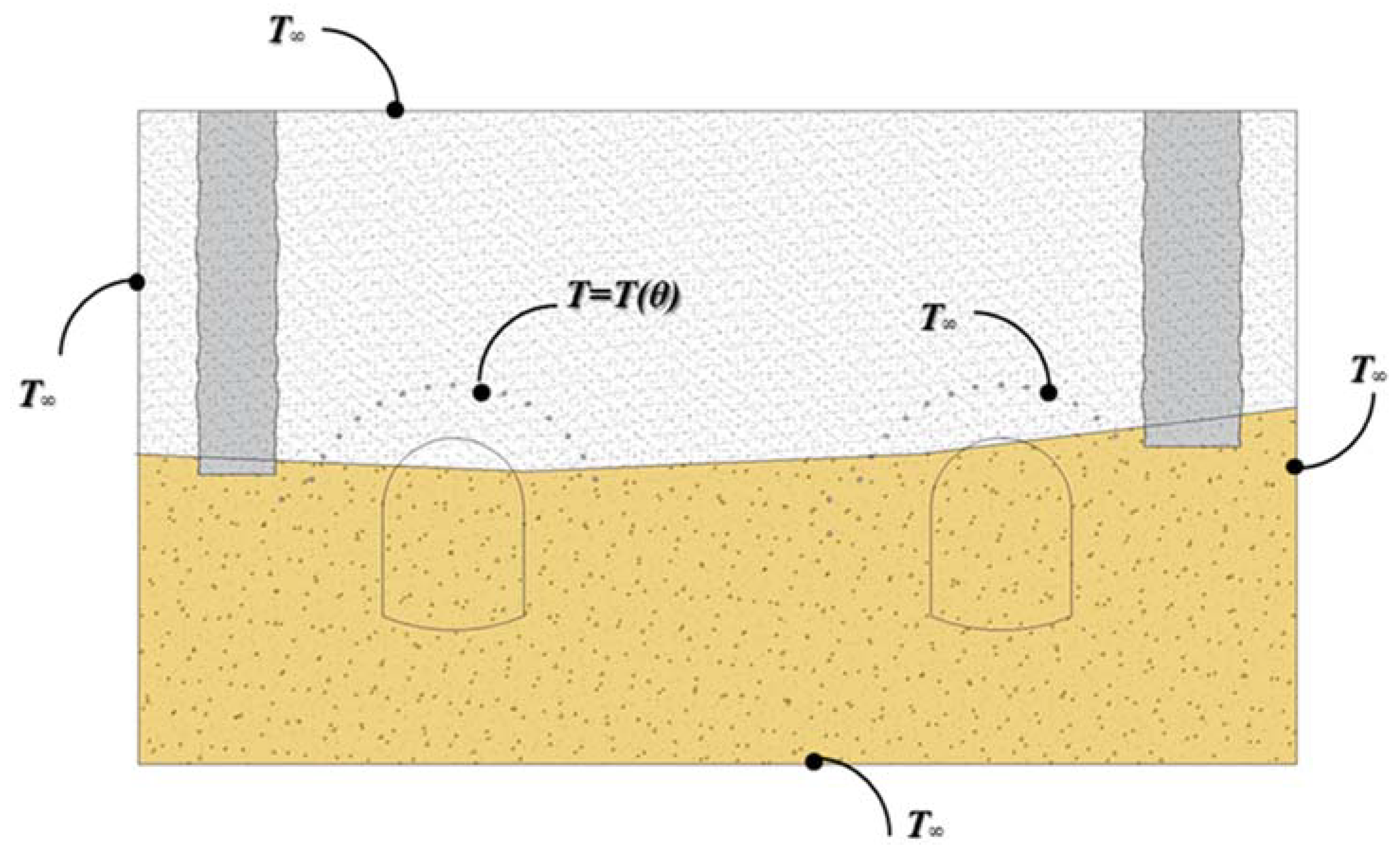
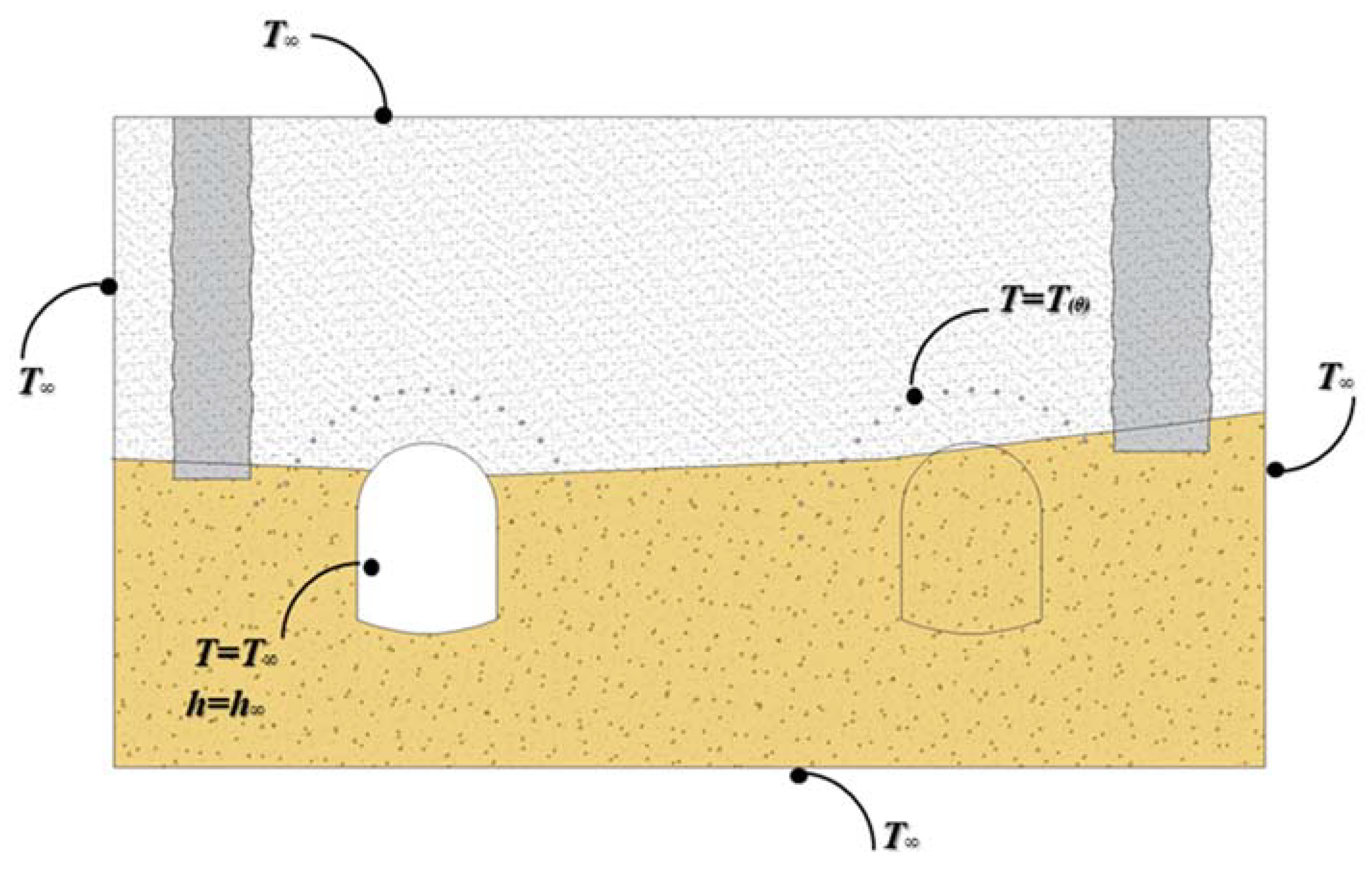
The boundary conditions employed in the present model refer to the soil and probes domain and are sketched in
Figure 7 and
Figure 8. In particular,
Figure 7 refers to the domain considered before excavation of the first tunnel, while
Figure 8 refers to the domain considered after excavation of the first tunnel. The temperature of the top, bottom and lateral surfaces of the soil has been assumed to be constant during the analysis, equal to the average yearly temperature of the site under investigation,
16 °C.
As previously specified, due to the complexity of nitrogen phase change phenomena occurring inside the freezing probes, a linear temperature profile has been assumed for the refrigerant fluid between the inlet and outlet sections of the probes (refer to
Figure 5).
The temperature boundary conditions applied on the external perimeter of each probe depend on the phase of the freezing process. During “Phase 1-Nitrogen”, the temperature has a linear variation along the axis, from −196 °C to −110 °C, as shown in
Figure 5. During “Phase 2-Waiting”, the adiabatic condition,
, has been imposed on the probe boundary.
During “Phase 3-Brine”, the temperature of the probe boundary has been imposed equal to the temperature of the brine, −33 °C, in all the sections of the excavation.
In order to simulate the excavation of the even tunnel, the same steps employed for that of the odd tunnel have been considered. During these phases, the excavated odd tunnel (left) has been reproduced by eliminating the corresponding domain of soil and applying a proper boundary condition (refer to
Figure 8). This condition takes into account the presence of men, vehicles and air circulation in the excavated tunnel, and is represented by convective heat transfer on the walls of the odd tunnel:
where
is equal to 30 °C.
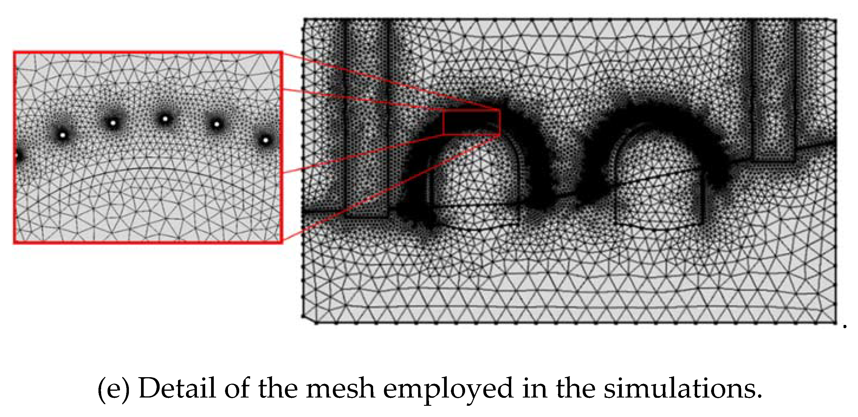
3.4. Mesh Sensitivity Analysis
A mesh sensitivity analysis has been carried out in order to obtain grid-independent numerical results. A domain of 20 × 25 m
2 has been considered. All the computational grids are made by triangular quadratic elements, and are refined near the freezing probes (
Figure 9).
Table 2 reports the details of the eight grids considered, together with a summary of the main numerical results. In particular, considering the nitrogen activation (phase 1), the days required for the formation of the frozen wall at 1.5 m have been calculated and reported in
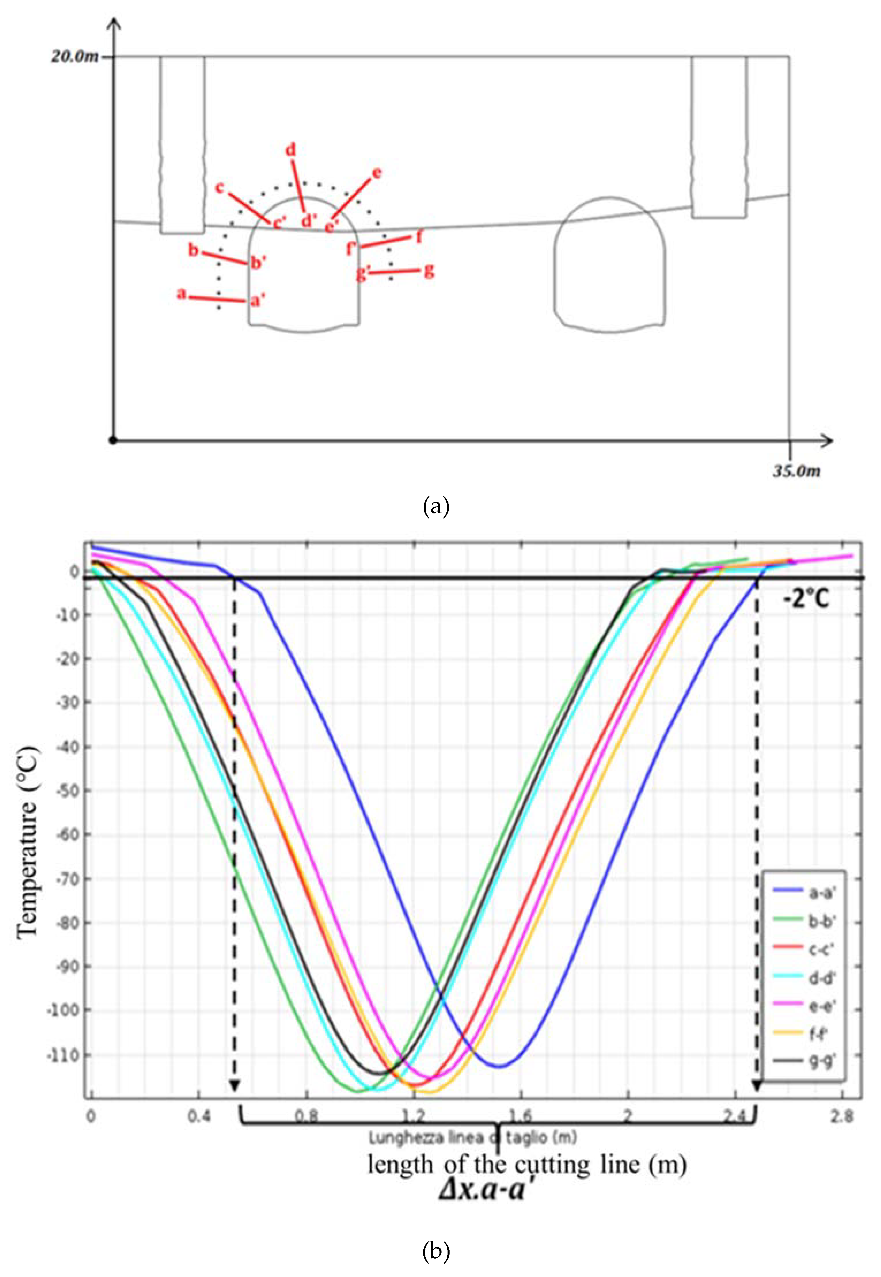
Table 2, together with the computing time necessary to reach the convergence. The nitrogen freezing phase is stopped when the desired design value of the frozen wall thickness is reached. The evolution of the frozen wall can be monitored, controlling the temperature of the ground at 0.5 m from the probe axis, which generally must be around −10 °C. Therefore, in the analysis, the temperature at this point has been taken into account.
On the basis of the present sensitivity analysis, the grid employed for the calculations is the one with 103,482 elements (letter f in the table), since the difference between the results obtained by using this grid, and the ones obtained by using the most effective adaptive grid, is around 1%.
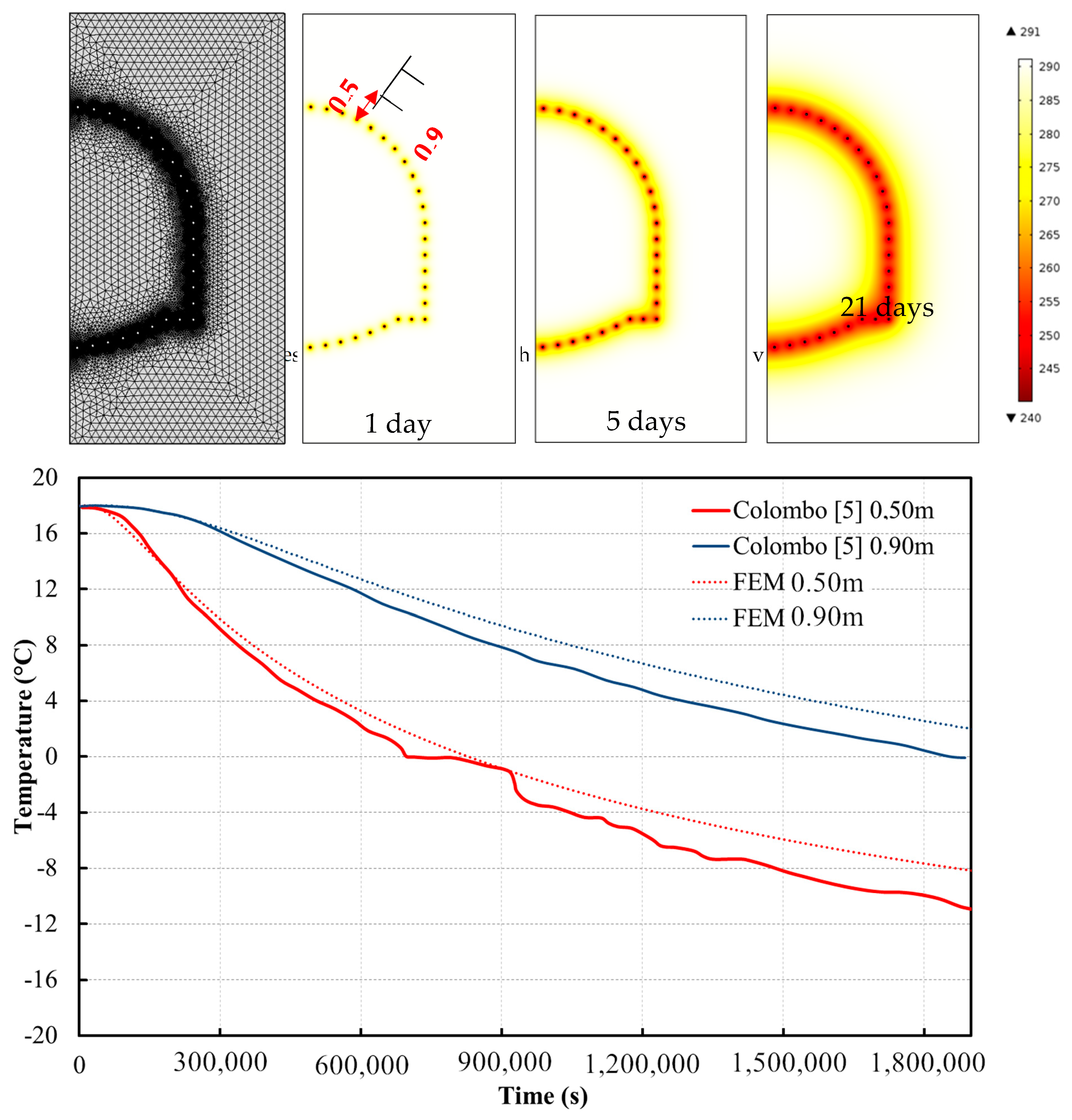
4. Model Validation
The present model has been validated against the numerical data reported by Colombo [
5], which is validated with on-field data. In that study, the software ABAQUS was used to solve the numerical model, and the computational domain was meshed by using DC2D4 elements. The geometry of the tunnel was symmetric. The present study reproduces the case study of Colombo [
5], based on a 2D model, by taking into account a computational domain representative of a portion of land equal to 10 × 20 m. A mesh consisting of 33,605 triangular elements has been considered, and the thermal characteristics of the materials are those reported in Colombo [
5], in particular: volumetric heat capacity of 1910 kJ/m
3K and 3100 kJ/m
3K for solid and liquid phases, respectively; thermal conductivity of 3.07 W/mK and 1.48 W/mK for the solid and liquid phases, respectively; volumetric latent heat of 179,280 kJ/m
3 and a saturated tuff density of 1550 kg/m
3. The initial temperature has been assumed equal to 18 °C, and the analysis has been carried out, imposing a linear variation of temperature down to −33 °C for the first day, on the nodes representing the perimeter of the freezing probe. In order to compare the results obtained from the present FEM analysis with those reported in Colombo [
5], the authors have considered two points located on a line orthogonal to the junction between the probes, at 0.50 m and 0.90 m.
Figure 10 shows the conditions that determine the propagation velocity of the freezing front in the tuff, evaluated for two points located at 0.5 m and 0.9 m from the freezing probe. It is evident that the temperature gradually decreases over time, and that a good agreement between the present numerical results and those available in the literature [
5] is observed.
6. Conclusions
This work presents an analysis of the heat transfer phenomena occurring during the artificial ground freezing (AGF) process on the actual case study of the tunnels between Line 1 and Line 6 of the Underground station in Piazza Municipio in Napoli, southern Italy. An efficient numerical model, based on conductive heat transfer and water phase change, has been developed and validated against the data available in the literature.
The present model has us allowed to simulate, for the first time in the literature, a mixed-method used for the freezing process from the first phase, based on the use of nitrogen, a maintenance phase that allows us to raise the temperature of the probes, and a third phase that involves the use of brine. The numerical model has allowed us to reproduce the evolution of the temperature field during the whole excavation process. The model has been used to illustrate the heat transfer phenomena associated with the phase change and the influence of latent heat, the influence of phase change, and temperature variation.
The present modeling activity allows us to identify the possible solutions for reducing the time required for the completion of the excavation activities and the freezing of the galleries. In addition to properly planning the nitrogen feeding phase, this approach allows the analysis of alternative solutions to accelerate the freezing of the soil, such as increasing the number of probes, or using different configurations.
The results show that the time needed to complete the freezing process and excavation of the two tunnels, consists of 120 days. Instead, 14 days are required to obtain an ice vault with a thickness larger than the minimum value required for safety reasons (1.5 m). In particular, the section that first reaches the formation of the frozen wall is the one at 5 m from the well of Line 6, and from this section, the excavation operations can begin. Moreover, the defrosting phase for the odd tunnel starts after 60 days, and after 90 days, the temperature rises up to 0 °C.
The authors believe that the present model is useful to optimize the AGF technique, and to better understand the heat transfer phenomena occurring between probes and ground.

 ,
, 


