A Decentralized Optimization Strategy for Distributed Generators Power Allocation in Microgrids Based on Load Demand–Power Generation Equivalent Forecasting

Abstract

In order to guarantee the economic and reliable operation of renewable Distributed Generators (DGs) in microgrids, a decentralized optimization strategy for DGs power allocation is proposed in this paper. According to the method, all processes and parameters are designed in a fully distributed way. To achieve decentralization and to maintain the balance between power supply and load demand, a load demand–power generation equivalent forecasting method is proposed to improve the strategy through replacing information of load demand by predicted power output, which removes the load prediction center and load sensor devices. The data of historical power generation, which is used for prediction, has already satisfied the balance constraint between power supply and load demand. Therefore, when the balance between the real power output and the predicted power output is gained, the balance constraint of power supply and load demand is achieved. Meanwhile, the uncertainty and forecasting errors of renewable generation are taken into account in the cost functions to optimize the expense of DG operation comprehensively. Then, the proposed algorithm is expounded in detail and the convergence is proved by eigenvalue perturbation theory. Finally, various cases are simulated to verify the accuracy and effectiveness of the proposed method. In summary, the proposed method are effective tools for DGs economic power allocation and the decentralization of microgrid system.

1. Introduction

To cope with the serious anthropogenic climate change and to decrease greenhouse gas emissions, more and more renewable energy sources are being applied in the advanced microgrid [1]. Hence, the management of renewable energy sources to guarantee microgrids operating economically and reliably becomes an essential issue, which has drawn great attention from researchers in various areas. Particularly, the question ‘to centralize or to decentralize’ is a highlight on the control and management of microgrids. The centralized optimization algorithms require global information of the whole system, which deeply depend on the control center. With the rapid increasing number of Distributed Generator (DG) units, the centralized methods are not suitable for a large-scale network, due to significance communications and massive computational overhead. Such disadvantages motivate researches on decentralized optimization methods. Literature [2] discussed and reviewed the state-of-the-art solutions regarding Micro Grid Management System (MGMS) in the primary, secondary, and tertiary levels, and drew a conclusion that the decentralized MGMS framework delivers not only the same control function as the centralized one, but also be with greater scalability, reliability, and resiliency. Meanwhile, the “plug and play” [3] demand of DG drives the tendency toward decentralization as well.

At present, decentralized optimization algorithms mainly depend on consensus or multi-agent systems. Each node/agent in a system only concerns about local decision variables instead of global information, and neighboring nodes/agents communicate with each other to cooperate together for achieving optimization results [4]. For example, a multi-agent system-based hierarchical control method was applied in autonomous microgrids for cooperative frequency control with communication constraints [5]. A state-based consensus method [6] was proposed, which made use of the state information of DGs to calculate the optimized dispatching strategy under a layered architecture. However, such methods still rely on the control center to collect the information and to send to each DG. To fully decentralize the optimization and to remove the control center, Ref. [7] proposed a consensus-based approach for economic dispatch problems in a smart grid without any center or leaders. On this basis, Ref. [8] proposed a distributed algorithm to solve the resource allocation over dynamic digraphs, which is adaptable to the scenario under the time-varying graph. Noticeably, all of the above methods required the information of total load demand in a microgrid to keep the balance constraint between power supply and load demand in the optimization. Moreover, to consider the impact of load on the cost optimization, Refs. [9,10,11] established the utility function of each load. However, the total load demand information was gained through load forecasting [12], which depended on a prediction center. Hence, the center restrains the decentralization faith. In addition, the setting-up of utility function of each load needs distributed loads’ information, which requires setting sensors at each load. It is difficult to implement in large-number and distributed load scenarios. Therefore, an effective measure should be carried out to solve the above problem.

Meanwhile, the cost function in the decentralized optimization is always treated as a simple quadratic polynomial function. For example, the consensus iterative algorithm based on bias feedback dynamic adjustment method was proposed in [13] for distributed robust economic dispatch. A method relaxed hybrid consensus Alternating Direction Multiplier Method (ADMM) with coupling constraints was proposed in [14] for distributed convex optimization. They all ignored the uncertainty of renewable DGs influencing on the expense. Since the uncertainty is mainly due to randomness and volatility of wind/photovoltaic power, the optimization of MGMS needs to consider the uncertainty of DGs in the cost function. In [15,16,17], authors analyzed probabilistic forecasting generation of wind turbine (WT) and photovoltaic (PV) power through machine learning during the optimization. However, authors did not analyze the effect of forecasting error on the cost function.

To address the mentioned challenges and to realize the economic and reliable operation of DGs in a microgrid, a decentralized optimization strategy for DGs power allocation basing on load demand–power generation equivalent forecasting is proposed in this paper. The main contributions of this paper are illustrated as follows.

• All processes and parameters of the proposed decentralized optimization strategy are designed in a fully distributed way, which do not need any center or leader to assign global variables or parameters. Each DG only needs to communicate with its neighbors under sparse communication to reach the optimal results.
• A load demand–power generation equivalent forecasting method is proposed to improve the decentralized optimization strategy, which replaces the load prediction center and the load sensor devices. The balance constraint only needs information of predicted power output instead of load demand. The historical power generation data, which is used for prediction, has already satisfied the balance constraint of power supply and load demand. When the sum of real power output equals to the sum of predicted output, the balance between power supply and load demand is achieved.
• The uncertainty of renewable generation is considered in the cost modeling process to optimize the expense comprehensively. A penalty term is introduced into the cost model for adjustment of the expense cost by the fluctuation of renewable energy sources and the forecasting error.

The remainder of this paper is outlined as follows. Section 2 introduces the DGs power allocation problem formulation and mathematical model. In Section 3, the decentralized optimization algorithm is presented and proved to be convergent. In Section 4, the accuracy and characteristic of the proposed method are verified through simulations, and compared with a centralized method. Then, the daily optimization results are analyzed to verify the effectiveness of the strategy. Finally, findings are concluded in Section 5.

2. Load Demand–Power Generation Equivalent Forecasting Based Distributed Generators (DGs) Power Allocation Strategy Formulation

The structure of DGs power allocation strategy, including construction, optimization objective, and algorithm, are shown in Figure 1.

• As mentioned in Section 1, the centralized optimization algorithms deeply depend on the control center, which requires collecting global information from the whole network. With the rapid increasing number of DG units, those approaches are not suitable for a large-scale network, due to significance communications and massive computational overhead. On the contrary, decentralized optimization algorithms mainly rely on consensus or multi-agent systems, which merely need sparse communication with neighbor DGs to achieve information interaction and cooperation [18]. Therefore, the decentralized mode is more suitable to implement the optimization.
• The optimization problem is aiming at the minimum cost of the outputs of DGs. When the total outputs of DGs is determined, a ‘Power Allocation Strategy’ need to be studied to obtain the output of each DG unit. Thereby, we can get the accurate dispatching plan of each DG unit. The Power Allocation Strategy consists of the optimization objective and the optimization algorithm.
• A load demand–power generation equivalent forecasting method is proposed in the optimization algorithm, which only needs the information of predicted power output instead of load demand. The historical power generation data, which is used for prediction, has already satisfied the balance constraint of power supply and load demand. Therefore, when the balance between the real power output and the predicted output is gained, the equation constraint of power supply and load demand is satisfied. Thereby, the load demand information could be substituted by the predicted power generation in a local way.
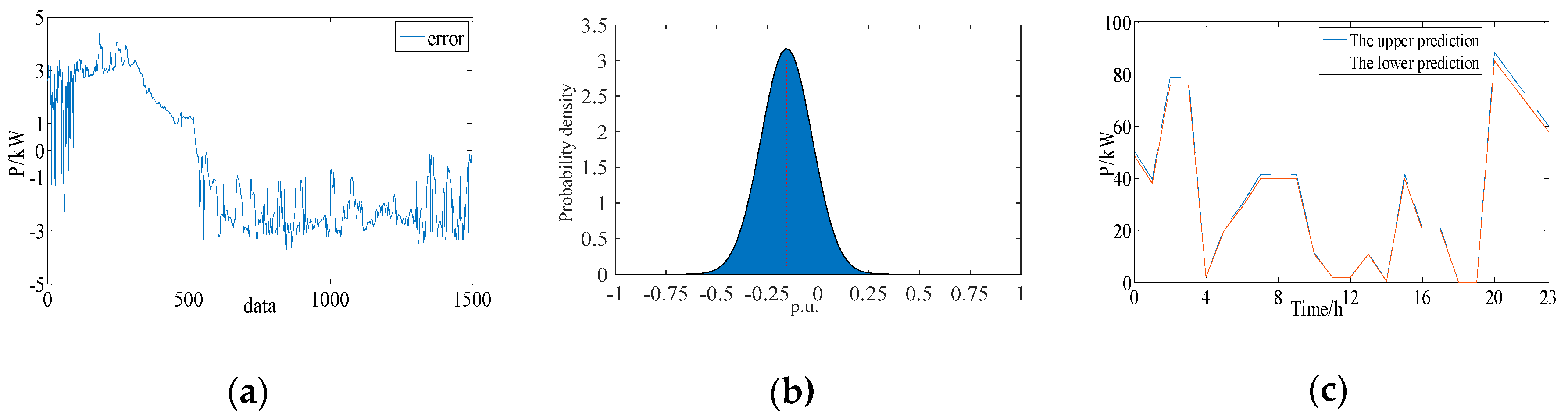
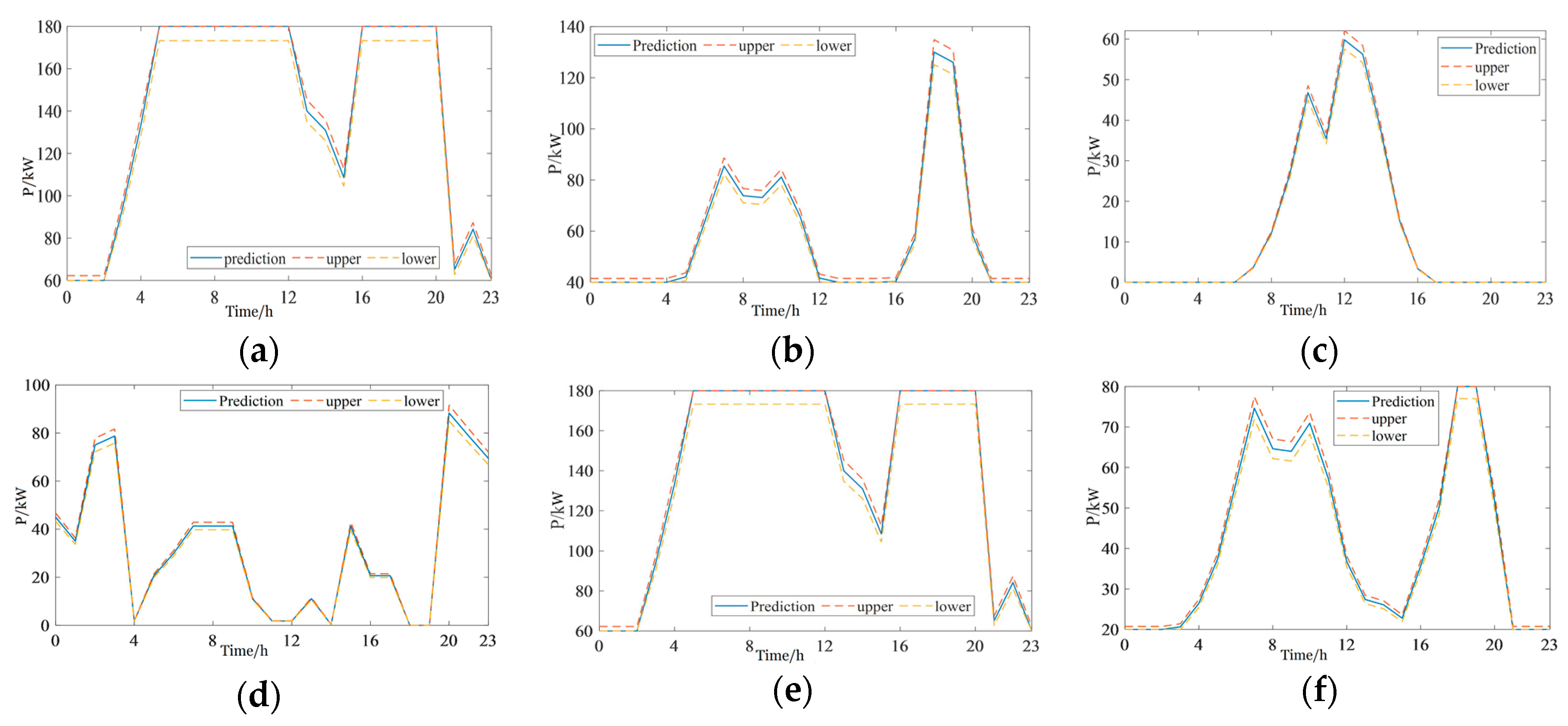
• Due to the uncertainty and fluctuation of the renewable energy sources, the prediction error is considered when gaining the predicted value for fitting a feasibility interval, and the real values of the predicted day are added to the training data to update the training process for a rolling optimization. Before establishing the model of optimization, the prediction method needs to be analyzed to support the optimization strategy.

2.1. Generation Output Prediction Interval Model

Since the short-term generation prediction of microgrid is a prediction of time series, Long Short-Term Memory Network (LSTM) is more suitable for generation prediction and is used for the prediction of DGs power output in this section. Take the short-term prediction neural network model of PV generation as an example. The impact factors of Photovoltaic (PV) generation, which are treated as input vectors, contain the historical power, light intensity, temperature, and humidity, as well as the temperature and humidity of the predicted day. Meanwhile, the final output of the prediction model is the predicted power of PV, with only one type of data. The neural network model is presented in Figure 2.

According to the above model, PV generation can be predicted. The prediction models for wind turbines, fuel turbines, and hydro turbines are built in a similar way. Some parameters for prediction of a typical region are shown in Figure 3. Figure 3a shows the annual historical temperature in the data collecting area. The annual output power of PV and WT are shown in Figure 3b,c (The data used is one sampling point per hour). It can be seen that the tested region is abundant with renewable energy resources and is suitable for the application of a microgrid system.

The predicted output of WT and PV on a typical day is obtained as shown in Figure 4a,b. We can clearly see that there exists error between the predicted value and the real value. Due to the high randomness and volatility of WT and PV output, the accuracy of prediction plays a vital role in the optimization process [19]. Thus, we take the forecasting error into consideration for a comprehensive optimization. As the fluctuation of WT is stronger, we chose 1500 data of the aimed device to test, which are shown in Figure 4c. We chose the predicted value ${\tilde{x}}_{i,t}^{†}$ as a reference value. As the existence of prediction error, the predicted value may not be the same as the real one. By comparing the error between the prediction value and the real one, it can be found that the error obeys a distribution law. According to the data distribution and the model in [17], we can assume that the error obeys a Gaussian distribution, which is defined as the mismatch between the real value and the predicted value $\Delta {\tilde{x}}_{i,t}^{}=x_{i,t}^{}-{\tilde{x}}_{i,t}^{†}$. Then, the probability density function can be modeled as follows.

$$f(\Delta {\tilde{x}}_{i,t})=\frac{1}{\sqrt{2\pi }{\sigma }_{i,t}}\exp (-\frac{{(\Delta {\tilde{x}}_{i,t}^{})}^2}{2{\sigma }_{i,t}^2}),$$

(1)

where ${\sigma }_{i,t}^{}$ is the variance; let $100(1-{\alpha }_{i,t})\%$ represent confidence level, and ${\alpha }_{i,t}$ is usually chosen as 0.05.

Based on the probability density function, we can get the corresponding confidence interval $\left[\Delta {\tilde{x}}_{i,t}^{down},\Delta {\tilde{x}}_{i,t}^{up}\right]$. When the prediction error is considered, the predicted output turns to be as follows.

$$\begin{array}{l}{\tilde{x}}_{i,t}={\tilde{x}}_{i,t}^{†}+\Delta {\tilde{x}}_{i,t},{\tilde{x}}_{i,t_{\min }}^{}\le {\tilde{x}}_{i,t}^{}\le {\tilde{x}}_{i,t_{\max }}^{},\\ {\tilde{x}}_{i,t_{\min }}^{}=\Delta {\tilde{x}}_{i,t}^{down}+{\tilde{x}}_{i,t}^{†},\\ {\tilde{x}}_{i,t_{\max }}^{}=\Delta {\tilde{x}}_{i,t}^{up}+{\tilde{x}}_{i,t}^{†}\end{array},$$

(2)

where, ${\tilde{x}}_{i,t}^{}$ is the ith DG predicted value (largest possibility value) when considering the prediction error.${\tilde{x}}_{i,t_{\min }}^{}$ and ${\tilde{x}}_{i,t_{\max }}^{}$ are the lower and upper boundaries of ${\tilde{x}}_{i,t}^{}$.

The error between the real value and the predicted value (1500 data) is presented in Figure 5a. From the analysis, the error distribution of WT obeys a Gaussian distribution and is treated as a p. u. value in Figure 5b. When the prediction error is considered, the output of WT becomes a possible range in Figure 5c.

2.2. Optimization Model and Formulation

2.2.1. Optimization Objective

In this section, the optimization objective is set as the minimum of the total operating cost. Thereby, the cost function is formulated as (3), which mainly includes fuel turbines (Fes), wind turbines (WTs), photovoltaic sets (PVs), and hydropower turbines (HTs).

$$\min F=\min ({\displaystyle \sum _{i=1}^N{F}_i}(x_{i,t}))={\displaystyle \sum _{i=1}^{N_1}{F}_i}(x_{i,t}^{pv})+{\displaystyle \sum _{i=1}^{N_2}{F}_i}(x_{i,t}^w)+{\displaystyle \sum _{i=1}^{N_3}{F}_i}(x_{i,t}^{fe})+{\displaystyle \sum _{i=4}^{N_4}{F}_i}(x_{i,t}^{HT})$$

(3)

where, $F$ is the cost of generation, which mainly contains the cost of real outputs of DG units; $F_i(x_{i,t})$ is the cost of ith DG output; $x_{i,t}^{}$ is the real output of ith DG at time t; $x_{i,t}^{pv}$, $x_{i,t}^w$, $x_{i,t}^{fe}$ and $x_{i,t}^{HT}$ are the real output of each PV, WT, Fe, and HT at time t in a microgrid, respectively; $N_1$, $N_2$, $N_3$ and $N_4$ are the number of each DGs, respectively. $N=N_1+N_2+N_3+N_4$.

2.2.2. Cost Functions and Constraints of DGs

In order to achieve the optimization objective in Section 2.2.1, the cost function of each DG is established as (4)–(7). Each DG is supposed to operate within the equation constraint of its own capacity and to keep the balance between load demand and power supply in the system.

The cost function of PV is defined as follows.

$$F_i(x_{i,t}^{pv})=a_i{x}_{i,t}^{pv}+{\epsilon }_i\frac{{({\tilde{x}}_{i,t}^{pv}-x_{i,t}^{pv})}^2}{{\tilde{x}}_{i,t_{\max }}^{pv}-{\tilde{x}}_{i,t_{\min }}^{pv}},$$

(4)

where $F_i(x_{i,t}^{pv})$ is the ith PV generation cost and $x_{i,t}^{pv}$ is the real output value of the ith PV at time t; $a_i$ is the cost coefficient;${\epsilon }_i$ is the penalty factor; ${\tilde{x}}_{i,t}^{pv}$ is the prediction value (considering prediction error) of the ith PV at the moment t; ${\tilde{x}}_{i,t_{\max }}^{pv}$ and ${\tilde{x}}_{i,t_{\min }}^{pv}$ are the upper and lower boundaries of ${\tilde{x}}_{i,t}^{pv}$.

The cost function of WT is defined as follows.

$$F_i(x_{i,t}^w)=b_i{x}_{i,t}^w+{\gamma }_i\frac{{({\tilde{x}}_{i,t}^w-x_{i,t}^w)}^2}{{\tilde{x}}_{i,t_{\max }}^w-{\tilde{x}}_{i,t_{\min }}^w},$$

(5)

where, $F_i(x_{i,t}^w)$ is the ith WT generation cost and $x_{i,t}^w$ is the real output value of the ith WT at time t; $b_i$ is the cost coefficient; ${\gamma }_i$ is the penalty factor; ${\tilde{x}}_{i,t}^w$ is the prediction output value of the ith WT at the moment t. ${\tilde{x}}_{i,t_{\max }}^w$ and ${\tilde{x}}_{i,t_{\min }}^w$ are the upper and lower boundaries of ${\tilde{x}}_{i,t}^w$.

Remark 1.

Due to the randomness and volatility of the WT and PV generation, the accuracy of the prediction results has a great impact on the optimization objective. Therefore, a penalty term is introduced into the model for adjustment. Specifically, the smaller deviation between the real value and the predicted value is, the smaller impact the penalty term gains. For example, when ${\tilde{x}}_{i,t}^{}=x_{i,t}^{}$, the penalty term is zero, which means the predicted value is identical to the real value. In (4), the cost function consists of the operation cost $a_i{x}_{i,t}^{pv}$ and punishment of the deviation ${\epsilon }_i\frac{{({\tilde{x}}_{i,t}^{pv}-x_{i,t}^{pv})}^2}{{\tilde{x}}_{i,t_{\max }}^{pv}-{\tilde{x}}_{i,t_{\min }}^{pv}}$. Since the mismatch between the predicted value and the real value could be positive or negative, both two possible scenarios have an effect on the expense. Therefore, ${({\tilde{x}}_{i,t}^{pv}-x_{i,t}^{pv})}^2$ is used to represent the error effect, which is easy to calculate as well. ${\tilde{x}}_{i,t_{\max }}^{pv}-{\tilde{x}}_{i,t_{\min }}^{pv}$ is the confidence interval of the predicted value as a constant. ((5) is the same as (4)).

The cost function of Fe is expressed as follows.

$$F_i(x_{i,t}^{fe})=d_i{}^{fe}{(x_{i,t}^{fe})}^2+e_i{}^{fe}{x}_{i,t}^{fe}+f_i{}^{fe},$$

(6)

where, $F_i(x_{i,t}^{fe})$ is the ith Fe generation cost and $x_{i,t}^{fe}$ is the real output of the ith Fe at time t; $d_i{}^{fe}$, $e_i{}^{fe}$, and $f_i{}^{fe}$ are the cost coefficients.

The cost function of HT is expressed as follows.

$$F_i(x_{i,t}^{HT})=d_i{}^{HT}{(x_{i,t}^{HT})}^2+e_i{}^{HT}{x}_{i,t}^{HT}+f_i{}^{HT},$$

(7)

where, $F_i(x_{i,t}^{HT})$ is the ith HT generation cost and $x_{i,t}^{HT}$ is the real output of the ith HT at time t;$d_i{}^{HT}$, $e_i{}^{HT}$, and $f_i{}^{HT}$ are the cost coefficient. As Fe and HT are stable equipment, the prediction effort will not wildly influence their total expense. Hence, no more punishment is needed.

In order to simplify the solution process, the above cost function is commonly selected as a quadratic polynomial function, which can be obtained by data fitting. Meanwhile, the following supply–demand balance equation constraint and capacity inequality constraints should be satisfied during optimization. The formula is identified as follows.

$${\displaystyle \sum _{i=1}^{N_1}(x_{i,t}^{pv})}+{\displaystyle \sum _{i=1}^{N_2}(x_{i,t}^w)}+{\displaystyle \sum _{i=1}^{N_3}(x_{i,t}^{fe})}+{\displaystyle \sum _{i=4}^{N_4}(x_{i,t}^{HT})}={\displaystyle \sum _{i=1}^{N_1}({\tilde{x}}_{i,t}^{pv})}+{\displaystyle \sum _{i=1}^{N_2}({\tilde{x}}_{i,t}^w)}+{\displaystyle \sum _{i=1}^{N_3}({\tilde{x}}_{i,t}^{fe})}+{\displaystyle \sum _{i=4}^{N_4}({\tilde{x}}_{i,t}^{HT})},$$

(8)

where ${\tilde{x}}_{i,t}^{pv}$, ${\tilde{x}}_{i,t}^w$, ${\tilde{x}}_{i,t}^{fe}$ and ${\tilde{x}}_{i,t}^{HT}$ are the prediction output of the ith PV, WT, Fe, and HT at time t, respectively.

Remark 2.

In this paper, the balance constraint equality only needs information of predicted power output instead of load demand. The historical power generation data, which is used for prediction, has already contained the balance constraint of power generation supply and load demand. Therefore, when the balance between the real power output and the predicted output is gained, the equation constraint of power supply and load demand is satisfied. Considering the prediction error, the upper and lower boundaries of the equation are calculated to provide a probability interval for the optimization results.

In addition, the cost function should meet the following inequality constraints as well.

$$\begin{array}{ll}\mathrm{PV}\mathrm{capacity}\mathrm{constraint}:& x_{i,t}^{pv}{}_{\min }\le x_{i,t}^{pv}\le x_{i,t}^{pv}{}_{\max },\\ \mathrm{WT}\mathrm{capacity}\mathrm{constraint}:& x_{i,t}^w{}_{\min }\le x_{i,t}^w\le x_{i,t}^w{}_{\max },\\ \mathrm{Fe}\mathrm{capacity}\mathrm{constraint}:& x_{i,t}^{fe}{}_{\min }\le x_{i,t}^{fe}\le x_{i,t}^{fe}{}_{\max },\\ \mathrm{HT}\mathrm{capacity}\mathrm{constraint}:& x_{i,t}^{HT}{}_{\min }\le x_{i,t}^{HT}\le x_{i,t}^{HT}{}_{\max }\end{array}$$

(9)

2.3. Optimization Solution

According to the optimal objective (3) and equality constraint (8), the Lagrangian function can be obtained as follows.

$$L=\min ({\displaystyle \sum _{i=1}^N{F}_i}(x_{i,t}))+{\lambda }_i\left[\begin{array}{l}{\displaystyle \sum _{i=1}^{N_1}({\tilde{x}}_{i,t}^{pv})}+{\displaystyle \sum _{i=1}^{N_2}({\tilde{x}}_{i,t}^w)}+{\displaystyle \sum _{i=1}^{N_3}({\tilde{x}}_{i,t}^{fe})}+{\displaystyle \sum _{i=4}^{N_4}({\tilde{x}}_{i,t}^{HT})}\\ -{\displaystyle \sum _{i=1}^{N_1}(x_{i,t}^{pv})}-{\displaystyle \sum _{i=1}^{N_2}(x_{i,t}^w)}-{\displaystyle \sum _{i=1}^{N_3}(x_{i,t}^{fe})}-{\displaystyle \sum _{i=4}^{N_4}(x_{i,t}^{HT})}\end{array}\right]$$

(10)

where L is the Lagrangian function and ${\lambda }_i$ is the Lagrangian multiplier of each DG.

Let $D={\displaystyle \sum _{i=1}^{N_1}({\tilde{x}}_{i,t}^{pv})}+{\displaystyle \sum _{i=1}^{N_2}({\tilde{x}}_{i,t}^w)}+{\displaystyle \sum _{i=1}^{N_3}({\tilde{x}}_{i,t}^{fe})}+{\displaystyle \sum _{i=4}^{N_4}({\tilde{x}}_{i,t}^{HT})}$. Then, the optimal conditions are provided by:

$$\{\begin{array}{l}\frac{\partial F}{\partial x_{i,t}^{pv}}=\frac{\partial F_i(x_{i,t}^{pv})}{\partial x_{i,t}^{pv}}-{\lambda }_i=0\\ \frac{\partial F}{\partial x_{i,t}^w}=\frac{\partial F_i(x_{i,t}^w)}{\partial x_{i,t}^w}-{\lambda }_i=0\\ \frac{\partial F}{\partial x_{i,t}^{fe}}=\frac{\partial F_i(x_{i,t}^{fe})}{\partial x_{i,t}^{fe}}-{\lambda }_i=0\\ \frac{\partial F}{\partial x_{i,t}^{HT}}=\frac{\partial F_i(x_{i,t}^{HT})}{\partial x_{i,t}^{HT}}-{\lambda }_i=0\\ \frac{\partial F}{\partial {\lambda }_i}=D-({\displaystyle \sum _{i=1}^{N_1}(x_{i,t}^{pv})}+{\displaystyle \sum _{i=1}^{N_2}(x_{i,t}^w)}+{\displaystyle \sum _{i=1}^{N_3}(x_{i,t}^{fe})}+{\displaystyle \sum _{i=4}^{N_4}(x_{i,t}^{HT})})=0\end{array}$$

(11)

According to (11), we can get the functional relationship between the optimal output $x_{i,t}^{}$ and the Lagrangian multiplier ${\lambda }_i$ that

$$\frac{\partial F_i(x_{i,t}^{pv})}{\partial x_{i,t}^{pv}}=\frac{\partial F_i(x_{i,t}^w)}{\partial x_{i,t}^w}=\frac{\partial F_i(x_{i,t}^{fe})}{\partial x_{i,t}^{fe}}=\frac{\partial F_i(x_{i,t}^{HT})}{\partial x_{i,t}^{HT}}={\lambda }_i,$$

(12)

Therefore, the Lagrangian multiplier ${\lambda }_i$ can be treated as the consensus variable, which communicates between each DG. Moreover, when ignoring the inequality constraints, there is a linear function relationship between ${\lambda }_i$ and $x_{i,t}^{}$, which can be represented as ${\varphi }_i({\lambda }_i)=x_{i,t}^{}$. When each DG is operating in the optimal consistent condition ${\lambda }_i{}^{\ast }$, the optimal power output $x_{i,t}^{\ast }$ can be obtained [20].

When considering the inequality constraints, the optimal conditions are written as follows.

$${\varphi }_i{}^{\ast }({\lambda }_i)=\{\begin{array}{l}{\overline{x}}_{i,t}^{},\mathrm{if}{\lambda }_i>{\overline{\lambda }}_i\hfill \\ x_{i,t}^{\ast },\mathrm{if}{\underset{\_}{\lambda }}_i\le {\lambda }_i\le {\overline{\lambda }}_i\hfill \\ {\underset{\_}{x}}_{i,t}^{},\mathrm{if}{\lambda }_i<{\underset{\_}{\lambda }}_i\hfill \end{array}$$

(13)

where ${}^{\ast }$ means the optimal condition; ${\overline{x}}_{i,t}^{}$ and ${\underset{\_}{x}}_{i,t}^{}$ represent $x_{i,t}^{}{}_{\mathrm{m}\mathrm{ax}}$ and $x_{i,t}^{}{}_{\min }$, respectively. $\overline{\lambda }={\varphi }^{-1}({\overline{x}}_{i,t}^{})$ and ${\underset{\_}{\lambda }}_i={\varphi }^{-1}({\underset{\_}{x}}_{i,t}^{})$.

3. The Decentralized Optimization Method Analysis

In this section, the decentralized optimization method is proposed to deal with the problem formulated in Section 2. The method is presented without capacity constraints firstly, and generalized to the situation with constraints. Then, the proof of convergence and the flow of the proposed algorithm are explained in this section. Before elaborating details of the proposed method, some preliminary knowledge is presented briefly.

3.1. Preliminary Knowledge

3.1.1. Graph Theory

Considering a microgrid with N DGs, a digraph $\zeta =(\nu ,\epsilon ,A)$ is used to model the network topology of the system based on the communication infrastructure [21]. The digraph consists of a nonempty finite nodes set $\nu =\left\{1,\cdots ,i,\cdots N\right\}$, and a finite edges set $\epsilon =\left\{(i,j)\right\}\subseteq \nu \times \nu$ which means DG j can receive information from DG i. $A$ is the adjacency matrix. When every node in the digraph is reachable from others, $\zeta$ is said to be strongly connected. Moreover, for each node $i\in \nu$, the sets of in-neighbors are denoted as $N_i^{+}=\left\{j\in \nu |(j,i)\in \epsilon \right\}$, and out-neighbors are $N_i^{-}=\left\{j\in \nu |(i,j)\in \epsilon \right\}$. Note that $N_i^{+}\ne N_i^{-}$ generally. Let $d_i^{+}=\left|N_i^{+}\right|$ and $d_i^{-}=\left|N_i^{-}\right|$ be the in-degree and out-degree of node i, respectively. In a strongly connected digraph $d_i^{+}\ne 0$ and $d_i^{-}\ne 0$.

3.1.2. The Design of Communication Weight

Let us define two matrices $W,U\in {\mathbb{R}}^{N\times N}$ associated with the digraph $\zeta =(\nu ,\epsilon ,A)$ as follows.

$$\begin{array}{c}{W}_{i,j}=\{\begin{array}{ll}\frac{1}{d_i^{+}}\hfill & ,\mathrm{if}j\in N_i^{+}\hfill \\ 0\hfill & ,\mathrm{otherwise}\hfill \end{array}\forall i,j\in v.\\ U_{i,j}=\{\begin{array}{ll}\frac{1}{d_i^{-}}\hfill & ,\mathrm{if}j\in N_i^{-}\hfill \\ 0\hfill & ,\mathrm{otherwise}\hfill \end{array}\forall i,j\in v.\end{array}$$

(14)

Based on the definition of communication matrices, it is clear to gain that $W_{i,j}$ is a row stochastic matrix and $U_{i,j}$ is a column stochastic matrix. Note that the convergence will not be affected by the communication weights selection process when the above stochastic characteristics are satisfied [20]. Note $\rho (W)=\rho (U)=1$, where $\rho (\cdot )$ represents the spectral radius of the matrix.

3.1.3. Assumptions and Lemmas

The proposed method should be subjected to the following assumption and lemmas, for convergence.

Assumption 1.

The digraph $\zeta =(\nu ,\epsilon ,A)$ is strongly connected.

When the digraph is strongly connected, every node in the digraph is reachable from others. Then, it can make sure that the global accessibility of the information which requires communication.

Lemma 1

([8]). The weight matrices $W$, $U$ satisfy the following:

1. 

1is a right eigenvector of all$W_{}$,$W_{}1=1$and$\underset{k\to \infty }{\lim }{W}^k=1w^T,w>0\mathrm{and}{1}^{T}w=1.$

2. 

1 is a left eigenvector of all $U$, $1^{T}U=1^T$ and $\underset{k\to \infty }{\lim }{U}^k=\mu 1^T,\mu >0\mathrm{and}{1}^T\mu =1.$

where 1 denotes a vector with all elements being 1 at length N.

Lemma 2.

The cost function $F$ of each DG is twice continuously differentiable in R (the set of real number) and the second derivative is a real number $l_i$.

$$\frac{\partial F^2\left(x_{i,t}^{}\right)}{\partial x_{i,t}^2}=l_i,\forall {\underset{\_}{x}}_{i,t}^{}<x_{i,t}^{}<{\overline{x}}_{i,t}^{}.$$

(15)

Proof of Lemma 2.

According to (4)–(7), it can be verified that (6) and (7) meet Lemma 2. Then, the cost function (4) consists of the operation cost and the punishment of deviation. Obviously, the operation cost $a_i{x}_{i,t}^{pv}$ is consistent with Lemma 2. For the punishment of deviation, ${\tilde{x}}_{i,t}^{pv}$ and ${\epsilon }_i$ are treated as constants. Then, Equation (4) can be treated as quadratic polynomials, which is submitted to Lemma 2 as well. (Equation (5) is the same as (4)). □

3.2. Consensus-Based Optimization Algorithm

Definition 1.

$$\begin{array}{l}{\lambda }_i(k+1)={\lambda }_i(k)+\left[{\displaystyle \sum _{j\in N_{{}_i}^{+}(k)}{W}_{i,j}}({\lambda }_j(k)-{\lambda }_i(k))\right]+\eta y_i(k)\\ x_i(k+1)=\varphi ({\lambda }_i(k+1))\\ y_i(k+1)={\displaystyle \sum _{j\in N_{{}_i}^{+}(k)}{U}_{i,j}}{y}_j(k)-(x_i(k+1)-x_i(k))\end{array}$$

(16)

where ${\lambda }_i(k+1)$ is the consensus variables of the communication between each DG; $x_i(k+1)$ is the output of DG; $y_i(k+1)$ is the mismatch between the total predicted output and the total real output, which is used as a feedback to adjust the iteration dynamically. $W_{i,j}$ and $U_{i,j}$ are the communication weights defined in (14). $\eta$ is a sufficiently small positive constant gain for mismatch term.

Remark 3.

As $W_{i,j}$ is a row stochastic matrix, the iteration could be written as ${\lambda }_i(k+1)={\displaystyle \sum _{j\in N_{{}_i}^{+}(k)}{W}_{i,j}}{\lambda }_j(k)+\eta y_i(k)$. Although the two forms are mathematically equivalent, they have different physical interpretations. The form presented in (16) means that the state of consensus variable ${\lambda }_i$ at k + 1 is decided by not only the state of its neighbors at k, but also its own previous state at k.

Initialization: 

$$\{\begin{array}{l}{x}_i(0)=\Pi \hfill \\ {\lambda }_i(0)={\Pi }^{\prime }\hfill \\ y_i(0)=\{\begin{array}{c}{D}_i-x_i(0),ifi\in N_0^{-}\\ -x_i(0),ifi\notin N_0^{-}\end{array}\hfill \\ \forall i\in \nu \end{array}$$

(17)

where $D_i=\frac{D}{N}$, D is defined as the total value of the predicted output in Section 2. The estimation method enables the algorithm to get rid of a leader and the initialized value can be any fixed admissible values $\Pi$ and ${\Pi }^{\prime }$, without impact on the convergence.

3.3. Proof of Convergence

To analyze the convergence, rewrite (16) as the following matrix form:

$$\begin{array}{l}\lambda (k+1)=W(\lambda (k)+\eta y(k)\\ x(k+1)=\overline{L}(\lambda (k+1))+\tau \\ y(k+1)=Uy(k)-(x(k+1)-x(k))\end{array}$$

(18)

where, $x(k+1)=\overline{L}(\lambda (k+1))+\tau$ is the liner relationship form of $x_i(k+1)=\varphi ({\lambda }_i(k+1))$. Therein, $\overline{L}$ is a diagonal matrix with elements $l_i$, and $\overline{L}=\mathrm{diag}\left[l_1,l_2,\dots ,l_N\right]$. $\tau$ is a constant vector.$\lambda$,$x$, and $y$ are the column stack vectors of ${\lambda }_i$,$x_i$, and $y_i$.

According to Lemma 1, it can be verified that:

$$1^{T}y(k+1)=1^{T}Uy(k)-1^T(x(k+1)-x(k))=1^{T}y(k)-1^{T}x(k+1)+1^{T}x(k).$$

Therefore, $1^T(y(k+1)+x(k+1))=1^T(y(k)+x(k))$, which means that the sum of the mismatch and the real output keep constant with the predicted value. Then, replace all $x$ with $\lambda$. (19) turns to be:

$$\left[\begin{array}{c}\lambda (k+1)\\ y(k+1)\end{array}\right]=(\Gamma +\eta \Omega )\left[\begin{array}{c}\lambda (k)\\ y(k)\end{array}\right]$$

(19)

where, $\Gamma =\left[\begin{array}{cc}W& 0\\ \overline{L}(I-W)& U\end{array}\right], \Omega =\left[\begin{array}{cc}0& I\\ 0& -\overline{L}\end{array}\right]$.

It is easy to know that the eigenvalues of $\Gamma$ is the union of $W$ and $U$. According to lemma 1, $1w^T=1$ and $\mu 1^T=1$. $\Gamma$ has two eigenvalues which can be defined as ${\varpi }_1={\varpi }_2=1$. According to eigenvalue perturbation theory [22], two following matrices are constructed.

$$M=\left[\begin{array}{cc}{1}^T\overline{L}& 1^T\\ w^T& 0\end{array}\right],V=\left[\begin{array}{cc}0& 1\\ \mu & l\mu \end{array}\right]$$

(20)

where, $l={\displaystyle \sum _{i=1}^N{l}_i}$.

Then, we can gain that $MV=I$. The variation of ${\varpi }_1,{\varpi }_2$ can be quantified by the eigenvalues of $M\Omega V$, and

$$M\Omega V=\left[\begin{array}{cc}0& 0\\ w^T\mu & -l{w}^T\mu \end{array}\right]$$

(21)

We can get the conclusion $d{\varpi }_1/d\eta =0,d{\varpi }_2/d\eta =-l{w}^T\mu <0$ are two eigenvalues of $M\Omega V$, which proves that $d{\varpi }_1$ is not changing against $\eta$, and when $\eta >0$, $d{\varpi }_2$ becomes smaller. Therefore, there exists an upper boundary of $\eta$, enabling $\left|{\varpi }_2\right|<1$. Hence, all the rest of the eigenvector of the matrix are within the open unit disk. It can be proved that ${\left[1^T,0^T\right]}^T$ is the eigenvector of matrix $\Gamma +\eta \Omega$. Then we can get $y_i(k)\to 0,k\to \infty$ and ${\lambda }_i$ converges to a common value.

3.4. Generalization to Constrained Condition

When considering the inequality constraints, the algorithm (16) turns to the following form.

$$\begin{array}{l}{\lambda }_i(k+1)={\lambda }_i(k)+\left[{\displaystyle \sum _{j\in N_{{}_i}^{+}(k)}{W}_{i,j}}({\lambda }_j(k)-{\lambda }_i(k))\right]+\eta y_i(k)\\ x_i(k+1)={\varphi }^{}({\lambda }_i(k+1))=\{\begin{array}{l}{\overline{x}}_{i,t}^{},\mathrm{if}{\lambda }_i>{\overline{\lambda }}_i\hfill \\ x_{i,t}^{},\mathrm{if}{\underset{\_}{\lambda }}_i\le {\lambda }_i\le {\overline{\lambda }}_i\hfill \\ {\underset{\_}{x}}_{i,t}^{},\mathrm{if}{\lambda }_i<{\underset{\_}{\lambda }}_i\hfill \end{array}\\ y_i(k+1)={\displaystyle \sum _{j\in N_{{}_i}^{+}(k)}{U}_{i,j}}{y}_j(k)-(x_i(k+1)-x_i(k))\end{array}$$

(22)

where the relationship between ${\lambda }_i(k+1)$ and $x_i(k+1)$ is treated as (13). The initial value can be set to any admissible value as well.

Initialization: 

$$\{\begin{array}{l}{x}_i(0)=\{\begin{array}{l}\begin{array}{cc}{\underset{\_}{x}}_i& if{\underset{\_}{x}}_i<\end{array}{D}_i\hfill \\ \begin{array}{cc}{D}_i& if{\underset{\_}{x}}_i<D_i<{\overline{x}}_i{}_i\end{array}\hfill \\ \begin{array}{cc}{\overline{x}}_i& if{D}_i>\end{array}{\overline{x}}_i\hfill \end{array}\hfill \\ {\lambda }_i(0)={\varphi }^{-1}(x_i(0))\hfill \\ y_i(0)=D_i-x_i(0)\hfill \\ \forall i\in \nu \hfill \end{array}$$

(23)

When ${\displaystyle \sum _{i=1}^N{\underset{\_}{x}}_i}\le D\le {\displaystyle \sum _{i=1}^N{\overline{x}}_i}$, at least one DG is not saturated. There still exists an optimization solution in this condition. Thus, this paper only considers the saturated case, which means taking into account the outputs as upper boundaries, where ${\displaystyle \sum _{i=1}^N{y}_i(k)}=D-{\displaystyle \sum _{i=1}^N{x}_i(k)}$ is the mismatch between the total generation supply and the load demand. $\eta$ is a feedback gain. ${\lambda }_i(k)$ will increase as k updates and converges to the same value. As the total power generation is a monotone increasing function of the incremental cost, the total amount of generation will increase as well. Therefore, the feedback item will reduce the mismatch. In this process, some DGs may reach its maximum capacity. Then, the DG output holds saturation after it gets saturated or after a sufficiently long time. Therefore, the communication weights of saturated DG is equivalent to $l_i=0$, and those unsaturated DGs will still participate in feedback adjustment until $y_i(k)\to 0,k\to \infty$ achieves convergence of the algorithm.

3.5. Solution Algorithm Flow

According to the discussion above, the algorithm flow is generated as shown in Figure 6. The specific steps are as follows.

Firstly, based on the multi-type data, the LSTM method is used to predict the generation of DGs locally.

Step 1. Collect historical generation data, regional meteorological information of the tested regional microgrid, including the historical power, light intensity, wind speed, temperature, and humidity. The sampling period is chosen as one hour a time, which collected a total of 24 points per day.

Step 2. Preprocess the collected data to form the training data set, which replaces outliers through the adjacent daily interpolation.

Step 3. Train the LSTM neural network model annually with training data set to ensure the LSTM neural network is retrained every year.

Step 4. Collect the information of the predicted day, including the light intensity, wind speed, temperature, and humidity of the predicted day. Use the trained LSTM and the information of the predicted day to predict the local generation of the DG in the regional micro grid including WT, PV, Fe, and HT. The prediction error is considered when gaining the predicted value for fitting a feasibility interval as illustrated in (2), and the real values of the predicted day are added to the training data to update the training process for a rolling optimization.

Secondly, combined with the results of power generation prediction, the decentralization optimization model is established. Moreover, the optimization model does not depend on the load information, which only needs the predicted the output. Therefore, local operations can be implemented without a control center.

Step 5. According to the solution of optimization method proposed in (12), define the consensus variable.

Step 6. Initialization—set the initial value of the optimization variable within the valid range.

Step 7. Enter the iterative calculation process. Define the communication weights required for the iteration according to the definition described in (14).

Step 8. According to the iteration strategy (22) update the optimal variables.

Step 9. Determine whether the result is within the constraint or not. If the result is beyond the limit, modify the variables under its constraints and go back to step 5; otherwise, go to the next step.

Step 10. Criticize whether the iteration is end or not. If the mismatch meets the convergence condition, stop the iteration and print the output; otherwise, continue to iterate until convergence.

4. Simulation and Case Study

In this section, several simulations under a text system with six DG units—A1, A2 … A6 are used to verify the accuracy of the proposed method. The communication topology is shown in Figure 7. Some parameters of DGs are listed in

Table 1. Simulation parameters.

DG Number	${\mathit{a}}_{\mathit{i}}$$/{\mathit{b}}_{\mathit{i}}$$/{\mathit{d}}^{\mathit{f}\mathit{e}}$$/{\mathit{d}}^{\mathit{H}\mathit{T}}$	$\mathit{\epsilon }$$/\mathit{\gamma }$$/{\mathit{e}}^{\mathit{f}\mathit{e}}$$/{\mathit{e}}^{\mathit{H}\mathit{T}}$	${\mathit{f}}^{\mathit{f}\mathit{e}}$$/{\mathit{f}}^{\mathit{H}\mathit{T}}$	${\overline{\mathit{x}}}_{\mathit{P}\mathit{g}}$ (kW)	${\underset{¯}{\mathit{x}}}_{\mathit{P}\mathit{g}}$ (kW)
A1 HT1	0.0184	3.5	15	180	60
A2 Fe1	0.1080	2.0	10	130	40
A3 PV	0.0087	1	/	150	0
A4 WT	0.0040	0.1	/	160	0
A5 HT2	0.0174	2.9	20	200	85
A6 Fe2	0.1250	1.8	25	80	20

A 1~6 are Hydro Turbine 1 (HT1), Fuel Turbine 1 (Fe1), Photovoltaic (PV), Wind Turbine (WT), Hydro Turbine 2 (HT2), and Fuel Turbine 2 (Fe2), respectively.

. The simulation results are obtained under MATLAB environment.

Based on Figure 7, the matrices $W$ and $U$ can be defined as

$$W=\left[\begin{array}{cccccc}\frac{1}{3}& 0& 0& \frac{1}{3}& 0& \frac{1}{3}\\ \frac{1}{3}& \frac{1}{3}& 0& 0& \frac{1}{3}& 0\\ 0& \frac{1}{3}& \frac{1}{3}& 0& 0& \frac{1}{3}\\ \frac{1}{3}& 0& \frac{1}{3}& \frac{1}{3}& 0& 0\\ 0& 0& 0& \frac{1}{2}& \frac{1}{2}& 0\\ 0& 0& \frac{1}{3}& 0& \frac{1}{3}& \frac{1}{3}\end{array}\right],U=\left[\begin{array}{cccccc}\frac{1}{3}& 0& 0& \frac{1}{3}& 0& \frac{1}{3}\\ \frac{1}{3}& \frac{1}{2}& 0& 0& \frac{1}{3}& 0\\ 0& \frac{1}{2}& \frac{1}{3}& 0& 0& \frac{1}{3}\\ \frac{1}{3}& 0& \frac{1}{3}& \frac{1}{3}& 0& 0\\ 0& 0& 0& \frac{1}{3}& \frac{1}{3}& 0\\ 0& 0& \frac{1}{3}& 0& \frac{1}{3}& \frac{1}{3}\end{array}\right]$$

respectively.

4.1. Verification of the Proposed Method

4.1.1. Verification of the Convergence

In this case, the convergence of the proposed method (22) is tested. As the time-scale is an hour, we chose an hour of a day randomly to operate the simulation. The simulation results—the optimal consensus variable ${\lambda }_i$, mismatch y_i, DGs output power x_i, and the sum of x_i are presented in Figure 7.

When the total predicted output D = 440 kW, the optimal solution is approximately ${\lambda }^{*}$ = 8.65. Obviously, all consensus variables (Lagrange multipliers) converge to the optimal value through the proposed algorithm. As shown in Figure 8a, they rise monotonously non-decreasing until the upper boundary (Note that $\lambda$ represents the incremental cost which is affected by the coefficient in the cost function). Figure 8b shows values of the feedback (mismatch) y of all DGs convergent to zero which proves that the mismatch is decayed with iteration. Figure 8c indicates the optimal power output. As shown in Figure 8d, the sum of the outputs of all DGs keep in balance with the total predicted value which meets the supply and demand constraints.

4.1.2. Verification of the Accuracy

To verify the accuracy of the proposed method, we chose the results of two single times to compare with the results achieved through the centralized method (quadratic programming). To gain a clearer observation, the values are presented in

Table 2. Results comparison.

DGs Serial Number	Time 1			Time 2
	M1	M2	P1	M1	M2	P1
A1 HT1	139.99	139.98	121.26	180	180	175.43
A2 Fe1	40	40	91.04	58.79	58.95	75.8
A3 PV	56.26	56.26	56.26	0	0	0
A4 WT	11.08	11.08	11.07	88.32	88.32	88.32
A5 HT2	165.27	165.27	140.14	200	200	189.44
A6 Fe2	27.40	27.41	20.21	51.60	51.73	50
Total	440	440	439.98	578.71	579	578.99

where, M1 is the proposed method; M2 is a central method (a quadratic programming); P1 is the predicted value. Time 1, 2 are two single times of a day. The output unit is kW.

. It can be seen that the result of the proposed method is very close to the centralized method. Meanwhile, the sum of DGs output equals to total prediction, which satisfies the balance condition proposed in Section 2. Thus, the optimization maintains the balance between power supply and load demand.

4.2. The Effect of Feedback Gain

The gain of the effect is the parameter that we need to manipulate, which plays an important role in the convergence speed and the performance. If the gain is not selected properly, the convergence will not be guaranteed. Thus, we chose four gains to test the performance, i.e., $\eta$ = 0.001, 0.005, 0.01, and 0.05. The results are shown in Figure 9.

Figure 9 shows that the mismatch y eventually converges to zero within the admissible value range. Noticeably, as $\eta$ increases gradually, the convergence speed rises up. Then, if $\eta$ keeps increasing until well beyond the range, the algorithm will not be convergent. For example, when $\eta \ge 0.1$, the operation loses stability. However, in this paper, the gain $\eta$ needs to have small parameters, which limits the convergence speed. In the future, a wilder parameter selection method and more relaxed convergent conditions will be studied.

4.3. Analysis of Daily Optimization Result on Hourly Time-scale

According to the data of the selected typical regions, the predicted output of DG can be obtained by the method proposed in 2.3, which can be used as the input data of the power balance constraint conditions during the decentralization optimization.

To analysis the distribution of the prediction error, 1500 data of the aimed device were chosen to test, which is shown in Figure 10a. We chose the predicted value as a reference value. By comparing the prediction value and the real one, we can obtain the error. Then, through fitting the data and observe the performance in Figure 10b, it can be found that the error obeys a Gaussian distribution and the error is less that 3.5 percent. When considering the prediction error, the possibility of the prediction values is illustrated in

Table 3. Prediction values of hours considering prediction error in a typical day.

DG	HT1	Fe1	PV	WT	HT2	Fe2
4 h	[78.69, 84.83]	[62.08, 66.92]	[0, 1.12]	[75.79, 81.69]	[96.16, 103.66]	[24.06, 25.94]
5 h	[116.71, 125.84]	[63.32, 68.25]	[0, 1.12]	[1.73, 1.86]	[144.37, 155.63]	[20.34, 21.93]
6 h	[163.63, 176.37]	[75.92, 81.84]	[0, 1.12]	[19.88, 21.43]	[173.35, 186.86]	[29.31, 31.59]
7 h	[173.25, 180]	[76.90, 82.89]	[0, 1.12]	[28.81, 31.06]	[192.5, 200]	[38.64, 41.65]
8 h	[163.62, 176.37]	[107.41, 115.77]	[3.40, 3.67]	[39.76, 42.86]	[192.5, 200]	[56.34, 60.73]
9 h	[163.63, 176.38]	[105.24, 113.44]	[11.73, 12.65]	[39.76, 42.86]	[172.28, 185.71]	[57.88,62.39]
10 h	[173.25, 180]	[78.56, 84.68]	[25.55, 27.54]	[39.77, 42.85]	[173.25, 186.75]	[72.68, 78.34]
11 h	[173.25, 180]	[100.91, 108.77]	[45.05, 48.56]]	[10.66, 11.49]	[192.5, 200]	[45.48, 49.03]
12 h	[173.25, 180]	[117.02, 126.14]	[34.08, 36.74]]	[1.73, 1.86]	[154, 166]	[39.66, 42.75]

Considering the error of prediction, the predicted values become a range rather than a level. In this area, before 6 a.m., the PV does not work. Thus, the results are illustrated from 4 a.m. to 12 p.m.

.

To analyze the characteristic of the simulation curves, the largest possibility values in the ranges were chosen as an example. The predicted outputs of DGs in a typical day are illustrated in Figure 11. Figure 12 presents the proportion of each DG among the total power generation.

Basing on the predicted outputs of each DG, the optimal power output can be gained by redistribution through the method proposed in Section 3.2. The results are shown in Figure 13 and Figure 14. As shown in Figure 13, when the prediction error is considered, the optimization results are turned to be a range of interval estimation, which is used to provide advice for day-ahead scheduling policies.

Through the bar chart in Figure 14, the sum of the outputs of each DG is consistent with the total predicted values, which is equivalent to the whole load demand. It can be clearly seen that there is strong uncertainty and volatility of the outputs of renewable energy generation. By contrast, hydro power and fuel turbine generation are more stable, which can be used for supporting the stability of a microgrid system. Therefore, when there is an increase in the proportion of renewable energy such as wind power, maintaining the system stable is one of highlights in current research. Meanwhile, the results are compared in

Table 4. Results comparison of hours in a day.

DG	Optimal Output (kW)
	4 h	5 h	6 h	7 h	8 h	9 h	10 h	11 h	12 h
HT1	93.99	133.43	180	180	180	180	180	180	180
Fe1	40	40	42.14	63.98	85.48	73.87	73.14	81.17	65.45
PV	0	0	0	0	3.54	12.19	26.54	46.81	35.41
WT	78.74	1.79	20.65	29.94	41.32	41.31	41.31	11.07	1.8
HT2	116.63	158.33	200	200	200	200	200	200	200
Fe2	20.63	26.44	37.21	56.08	74.66	64.62	63.99	70.93	57.35
Total	349.99	359.99	480	530	585	571.99	584.98	589.98	540.01
DG	Predicted Output (kW)
	4 h	5 h	6 h	7 h	8 h	9 h	10 h	11 h	12 h
HT1	81.76	121.26	170	180	170	170	180	180	180
Fe1	64.5	65.79	78.88	79.9	111.59	109.34	81.62	104.84	121.58
PV	0	0	0	0	3.54	12.19	26.55	46.82	35.41
WT	78.74	1.79	20.66	29.94	41.32	41.32	41.31	11.08	1.79
HT2	99.91	150	180.11	200	200	179	180	200	160
Fe2	25	21.14	30.45	40.15	58.54	60.14	75.51	47.26	41.21
D	349.91	359.98	480.10	529.99	584.99	571.99	584.99	590	539.99

The simple time is an hour. The data presented is from 4~12 h of one day. Total is the total of optimal output. D is the total of predicted output. The value is taken as the largest possibility value.

to gain a clearer observation.

In addition, it can be seen from the tendency of lines LD that the sum of the predicted value is consistent with the load demand. Specifically, the peak periods are from 6 a.m. to 12 p.m. and from 5 p.m. to 9 p.m. with larger load demand and power generation. The valley period is from 10 p.m. to 6 a.m. (the next day) and from 1 p.m. to 5 p.m. with smaller load demand and power generation. Meanwhile, to gain clearer observation, the values are presented in Table 4. We can see that the renewable generators WT and PV take the maximum use and the hydro power and the fuel turbines generation to adjust the mismatch flexibly aiming at the optimal objective—the minimum operation cost.

5. Conclusions

In this paper, a decentralized optimal operation method for DGs power allocation based on the equivalent forecasting is proposed. Firstly, a local generation prediction method was introduced into the decentralized optimization strategy to replace the load prediction center or the load sensor device. Based on the multi-type data, LSTM was used to predict the local power generation of each DG. Secondly, the uncertainty and prediction error of renewable generation was taken into account during the cost modeling process to optimize the expense comprehensively. Moreover, the system optimization model was improved based on the predicted power generation results, without load information, so that all process and parameters were designed in a fully distributed way. Then, the algorithm designing procedure was presented and the convergence was proved by eigenvalue perturbation theory. Finally, various cases are simulated and the effectiveness of the proposed method is verified.

However, during the research, there remains some questions requiring further study in the future.

• More types of equipment, such as energy storage devices and electric vehicles, are supposed to be considered during the operation optimization of a microgrid.
• Multi-energy utilizations, including cold, heat, power, and gas, should be introduced into the optimization model to fully maximize the benefit.
• The cost function in practice is more complex instead of a simple polynomial function form. It is usually non-convex, which is difficult to solve numerically. Therefore, a more widely applicable distributed solution algorithm needs to be studied in the future.

References

1. Strasser, T.; Andrén, F.; Kathan, J.; Cecati, C.; Buccella, C.; Siano, P.; Mařík, V. A Review of Architectures and Concepts for Intelligence in Future Electric Energy Systems. IEEE Trans. Ind. Electron. 2015, 62, 2424–2438. [Google Scholar] [CrossRef] [Green Version]
2. Cheng, Z.; Duan, J.; Chow, M. To Centralize or to Distribute: That Is the Question: A Comparison of Advanced Microgrid Management Systems. IEEE Ind. Electron. Mag. 2018, 12, 6–24. [Google Scholar] [CrossRef]
3. Huang, A.; Crow, M.L.; Heydt, G.T.; Zheng, J.P.; Dale, S.J. The Future Renewable Electric Energy Delivery and Management (FREEDM) System: The Energy Internet. Proc. IEEE 2011, 99, 133–148. [Google Scholar] [CrossRef]
4. Han, Y.; Zhang, K.; Li, H.; Coelho, E.A.A.; Guerrero, J.M. MAS-Based Distributed Coordinated Control and Optimization in Microgrid and Microgrid Clusters: A Comprehensive Overview. IEEE Trans. Power Electron. 2018, 33, 6488–6508. [Google Scholar] [CrossRef] [Green Version]
5. Liu, W.; Gu, W.; Sheng, W. Decentralized multi-agent system-based cooperative frequency control for autonomous microgrids with communication constraints. IEEE Trans. Sustain. Energy 2014, 5, 446–456. [Google Scholar] [CrossRef]
6. Divényi, D.; Dán, A.M. Agent-Based Modeling of Distributed Generation in Power System Control. IEEE Trans. Sustain. Energy 2013, 4, 886–893. [Google Scholar] [CrossRef]
7. Yang, S.; Tan, S.; Xu, J.X. Consensus based approach for economic dispatch problem in a smart grid. IEEE Trans. Power Syst. 2013, 28, 4416–4426. [Google Scholar] [CrossRef]
8. Xu, Y.; Han, T.; Cai, K.; Lin, Z.; Yan, G.; Fu, M. A distributed algorithm for resource allocation over dynamic digraphs. IEEE Trans. Signal Process. 2017, 65, 2600–2612. [Google Scholar] [CrossRef]
9. Ullah, M.H.; Alseyat, A.; Multi-Agent, J.P. System-based Distributed Energy Management in Smart Grid under Uncertainty. In Proceedings of the 2019 IEEE Energy Conversion Congress and Exposition (ECCE), Baltimore, MD, USA, 29 September–3 October 2019; pp. 3462–3468. [Google Scholar]
10. Yang, Z.; Wu, R.; Yang, J.; Long, K.; You, P. Economical operation of microgrid with various devices via distributed optimization. IEEE Trans. Smart Grid 2016, 7, 857–867. [Google Scholar] [CrossRef]
11. Zhang, H.; Li, Y.; Gao, D.W.; Zhou, J. Distributed optimal energy management for energy internet. IEEE Trans. Ind. Inform. 2017, 13, 3081–3097. [Google Scholar] [CrossRef]
12. Costa DA, C.; Otto, R.B.; Piardi, A.B.; Ramos, R.A. A Survey of State-of-the-Art on Microgrids: Application in Real Time Simulation Environment. In Proceedings of the 2019 IEEE PES Innovative Smart Grid Technologies Conference—Latin America (ISGT Latin America), Gramado, Brazil, 15–18 September 2019; pp. 1–6. [Google Scholar]
13. Kar, S.; Hug, G. Distributed robust economic dispatch in power systems: A consensus + innovations approach. In Proceedings of the IEEE Power and Energy Society General Meeting, San Diego, CA, USA, 22–26 July 2012. [Google Scholar]
14. Olama, N.; Bastianello, P.; Mendes, R.C.; Camponogara, E. Relaxed hybrid consensus ADMM for distributed convex optimisation with coupling constraints. IET Control Theory Appl. 2019, 13, 2828–2837. [Google Scholar] [CrossRef]
15. Wan, X.; Xu, Z.; Pinson, P.; Dong, Z.Y.; Wong, K.P. Probabilistic forecasting of wind power generation using extreme learning machine. IEEE Trans. Powers Syst. 2014, 29, 1033–1044. [Google Scholar] [CrossRef] [Green Version]
16. Ospina, J.; Newaz, A.; Faruque, M.O. Forecasting of PV plant output using hybrid wavelet-based LSTM-DNN structure model. IET Renew. Power Gener 2019, 13, 1087–1095. [Google Scholar] [CrossRef]
17. Chen, B.; Li, J. Combined probabilistic forecasting method for photovoltaic power using an improved Markov chain. IET Gener. Transm. Distrib. 2019, 13, 4364–4373. [Google Scholar] [CrossRef]
18. Olfati-Saber, R.; Fax, J.A.; Murray, R.M. Consensus and Cooperation in Networked Multi-Agent Systems. Proc. IEEE 2007, 95, 215–233. [Google Scholar] [CrossRef]
19. Zhang, J.; Cui, M.; He, Y. Robustness and Adaptability Analysis for Equivalent Model of Doubly Fed Induction Generator Wind Farm Using Measured Data. Appl. Energy 2020, 261, 114362. [Google Scholar] [CrossRef]
20. Ghamkhari, M.; Mohsenian-Rad, H. A Convex Optimization Framework for Service Rate Allocation in Finite Communications Buffers. IEEE Commun. Lett. 2016, 20, 69–72. [Google Scholar] [CrossRef]
21. Xiao, L.; Boyd, S. Fast linear iterations for distributed averaging. In IEEE Conference on Decision and Control; Elsevier: Amsterdam, The Netherlands, 2004. [Google Scholar]
22. Pagnier, L.; Jacquod, P. Optimal Placement of Inertia and Primary Control: A Matrix Perturbation Theory Approach. IEEE Access 2019, 7, 145889–145900. [Google Scholar] [CrossRef]
Figure 1. Structure of the microgrid system and optimization strategy.
Energies 13 00648 g001
Figure 2. Neural network model for Photovoltaic (PV) power generation prediction. where x ˜ i , t is represent the prediction output value. The input of model from P1 to P6 are historical power, light intensity, temperature, humidity and the temperature, humidity of the predicted day, respectively.
Energies 13 00648 g002
Figure 3. Annual historical temperature (a), Annual output power of PV (b), Annual output power of Wind Turbine (WT) (c).
Energies 13 00648 g003
Figure 4. PV output per hour (a), WT output per hour (b), WT Prediction and actual output of 1500 data (c).
Energies 13 00648 g004
Figure 5. The prediction error of WT (a), the error distribution in p. u. (b), comparison of WT output (c).
Energies 13 00648 g005
Figure 6. Optimization algorithm flow.
Energies 13 00648 g006
Figure 7. The communication topology of Distributed Generators (DGs).
Energies 13 00648 g007
Figure 8. The optimal consensus variable λ i (a), Mismatch y (b), DGs output power xi (c), the sum of xi (d).
Energies 13 00648 g008aEnergies 13 00648 g008b
Figure 9. The performance of mismatch when η = 0.001 (a), 0.005 (b), 0.01 (c), and 0.05 (d).
Energies 13 00648 g009aEnergies 13 00648 g009b
Figure 10. 1500 data of WT (a). The error distribution (b).
Energies 13 00648 g010
Figure 11. The predicted output of DGs.
Energies 13 00648 g011
Figure 12. Total power generation and load.
Energies 13 00648 g012
Figure 13. The optimal output of HD1 (a), The optimal output of FT1 (b), The optimal output of PV (c), The optimal output of WT (d), The optimal output of HD2 (e), The optimal output of FT2 (f).
Energies 13 00648 g013
Figure 14. Total power generation and load.
Energies 13 00648 g014