Abstract
The Time-Stepped Linear Superposition Method (TLSM) has been used previously to model and analyze the propagation of multiple competitive hydraulic fractures with constant internal pressure loads. This paper extends the TLSM methodology, by including a time-dependent injection schedule using pressure data from a typical diagnostic fracture injection test (DFIT). In addition, the effect of poro-elasticity in reservoir rocks is accounted for in the TLSM models presented here. The propagation of multiple hydraulic fractures using TLSM-based codes preserves infinite resolution by side-stepping grid refinement. First, the TLSM methodology is briefly outlined, together with the modifications required to account for variable time-dependent pressure and poro-elasticity in reservoir rock. Next, real world DFIT data are used in TLSM to model the propagation of multiple dynamic fractures and study the effect of time-dependent pressure and poro-elasticity on the development of hydraulic fracture networks. TLSM-based codes can quantify and visualize the effects of time-dependent pressure, and poro-elasticity can be effectively analyzed, using DFIT data, supported by dynamic visualizations of the changes in spatial stress concentrations during the fracture propagation process. The results from this study may help develop fracture treatment solutions with improved control of the fracture network created while avoiding the occurrence of fracture hits.
1. Introduction
Attempts to engineer the creation of fracture networks and their hydraulic conductivity are key for successful hydrocarbon field development strategies. To be successful, any hydraulic fracture intervention must consider the initial state of the reservoir (i.e., the local stress conditions, pore pressures, heterogeneities, anisotropy, stratification, faults, other natural fractures, and any pre-existing hydraulic fractures). A vast body of modeling attempts have focused on investigating how the various parameters affect the development of complex fracture networks during hydraulic fracturing [1,2]. Simultaneously, fracture characterization efforts in dedicated field experiments have revealed the existence of complex fracture networks in the vicinity of horizontal wells completed with multi-stage fracture treatment operations [3,4,5,6,7].
A number of key findings has come to the forefront from both the fracture characterization studies in field tests and the fracture propagation modeling work. Field observations from cores and micro-seismic monitoring have revealed that hydraulic fractures propagate as fracture swarms and do not necessarily remain transverse to the horizontal wellbores, even if the latter are aligned with the native minimum principal stress orientation [8]. Modeling work has shown that the fanning of hydraulic fractures occurs due to stress shadowing between the individual fractures as they propagate away from the perforation clusters during the fracture treatment operation. The fanning becomes increasingly suppressed when the far-field tectonic stress becomes increasingly anisotropic [9]. The interaction with the pre-existing natural fractures and parent well hydraulic fractures also greatly affects the development of the final fracture network from which the reservoir fluids are ultimately produced.
The topic of principal stress changes (and stress reversals) in the vicinity of hydraulically fractured wells has been studied in considerable detail, using a variety of fracture propagation simulators, especially focusing on the impact of a pre-existing parent-well fracture network on the development of infill-well fracture networks [2]. The occurrence of local stress deviations and the induced hydraulic fracture reorientation have been investigated in early experimental laboratory studies [10] and in field projects [11].
Previous studies have suggested that pore pressure is a primary cause for stress reversals that in turn control the subsequent hydraulic fracture re-orientation [12,13]. Micro-seismic results in Austin Chalk first pointed toward the occurrence of fracture reorientation, and suggested the involvement of stress reversals due to reservoir pressure depletion [14]. The reduction in pore pressure, resulting from compaction and subsidence due to production, would cause the reorientation of hydraulic fractures and the reversal of the principal stresses in the reservoir.
The present paper aims to determine in detail how and whether pore pressure and far-field stress superposition would, in fact, alter hydraulic fracture orientations. Our models of dynamic fracture propagation are based on the Linear Superposition Method (LSM) and the Time-Stepped Linear Superposition Method (TLSM). Both LSM and TLSM have been utilized in recent studies to evaluate stress concentration, stress reversal, and stress interference effects on the orientation of propagating hydraulic fractures [8,15,16,17]. The inclusion of poro-elastic effects is implemented in the present study, first for LSM (Section 3), and next for dynamic TLSM (Section 4.1 and Section 4.2). The latter expansion of TLSM can account for the local increase in pressures during diagnostic fracture injection tests (DFIT), scaled with field data (Section 4.3, Section 4.4 and Section 4.5). The effects of imposed pore pressure gradients are studied in Section 5, and discussion and conclusions are given in Section 6 and Section 7, respectively.
2. Pore Pressure and Localized Principal Stress Changes
What has remained perhaps poorly articulated in prior work is the careful distinction of the direct effect of pore pressure changes on (1) the local principal stress magnitudes, and (2) local principal stress orientations. First, the alleged changes in the orientation of principal stresses due to pore pressure alterations associated with engineering interventions are here grouped into Type A and Type B interventions. Type A intervention effects are short-term (days to weeks) and nearly instantaneous changes in the scalar reservoir pressure, accompanied by elastic strains in the rock adjacent to the main hydraulic fractures resulting in a local deviatoric stress tensor field, such as those induced by DFIT tests and full-blown fracture treatment operations. Type B intervention effects refer to the longer-term pressure changes (months to years) related to production-induced pressure depletion in the reservoir. When parent–child well situations are modeled, the effects of Type A and B interventions will start to interfere.
For example, the pressurization and depressurization of natural fractures due to injection and depletion in their vicinity can modify the magnitude of the in-situ stress. A hydraulic fracture propagation path due to Type A intervention would favor regions of higher local pore pressure, accompanied by locally increased tensile principal stress magnitudes that are superimposed on the in-situ stresses [18]. A nearby legacy or parent well, when being pressure-depleted due to a Type B intervention, may cause local changes in the stress magnitude as compared to the prior far-field stress magnitude. In the latter case, a reduction in the principal stress magnitude follows for a well under study. “Far-field stress” changes induced by an adjacent well may be a misnomer, and should be called “near-field stress” changes due to Type A and/or B interventions, as opposed to a regional native stress which traditionally is a familiar source of a “far-field stress”.
Re-completions and infill drilling with Type A interventions may alter the stress state in the reservoir by the generation of locally superposed principal stresses, changing the prior far-field stresses. Empirical evidence for this contention comes from the observation that hydraulic fractures during a re-fracturing process propagated normal to that of the initial hydraulic fractures [19]. This change was attributed to a change in the horizontal stress orientations during production. Based on the new results presented in our study, we claim that a 90 degree flip in fracture propagation direction is simply due to a switch in the minor and major principal stress directions, which can be induced by either over-pressuring or under-pressuring a formation with regional far field stresses. This phenomenon has been extensively studied for wellbores with overbalanced or underbalanced pressure loads [20,21,22,23].
Prior work has unequivocally established that induced shear stresses in rocks may cause the initially horizontal principal stress to reorient out of the horizontal plane and thereby influences the direction of subsequent fractures, which has been observed to be escalated in heterogeneous media [24]. However, such shear stresses cannot be generated by pore pressure changes, which is why we suggest that prior claims that the local principal stress reorientation would occur due to poro-elasticity seem untenable, as follows further from evidence from experiments presented in our study.
While pore pressure can change due to Type A and Type B interventions, it may not act as the primary mechanism for stress reversal and fracture reorientation. In practice, local changes in the prior far-field stress can be induced by a nearby, new child well is hydraulically pressured. Unlike the pore pressure change itself (which is a scalar quantity), the dilation of fracture planes causes elastic stresses that superimpose on a pre-existing stress state (which is a tensor quantity). Stress reversals, therefore, are not a primary, but rather a secondary effect of poro-elasticity, as these occur due to certain anisotropic “far-field” and “near-field” stress superposition situations. Examples will be shown in our study.
The ultimate goal of all modeling efforts on the reorientation of hydraulic fractures due to well interference, is to next plan the parent and infill-well placement in the field such that any stress reversals can be controlled to be conducive for fracture network development leading to production optimization [16,25]. If fracture hits between parent and chilled wells are to be avoided, insight from fracture development simulators are helpful [1,2]. The reorientation of hydraulic fractures and the occurrence of local stress reversals are suggested to be induced by concurring factors such as the propagation of hydraulic fractures, the presence of natural fractures that create local stress re-distributions interfering with the pre-existing far-field stresses.
3. Accounting for Poro-Elasticity in LSM and TLSM Models
Poro-elasticity is accounted for in this study by simple addition of the pore pressure multiplied by the Biot’s constant to the directional stress magnitude. The effect of pore pressure is shown to induce a change in the stress magnitude imposed by the hydraulic fractures on the elastic medium. Fundamental equations used in the Linear Superposition Method (LSM) and the Time-Stepped Linear Superposition Method (TLSM) are briefly outlined, and modified to model stress interference with poro-elasticity, first in this section. A geomechanical sign convention was employed to describe the magnitude of stresses for all model results. Henceforth, compressional stress magnitudes are positive, while tensional stress magnitudes are negative.
3.1. Method of Solution: LSM and TLSM
The static Linear Superposition Method (LSM) and dynamic Time-Stepped Linear Superposition Method (TLSM) have been recently developed and applied to model and visualize mechanical interactions between pressurized fractures [15] and boreholes [26]. TLSM and LSM are proposed as fast, gridless alternatives to commonly used, grid-dependent fracture propagation models, which are computationally more demanding and henceforth more expensive.
LSM was first introduced to model stress accumulations induced by boundary displacements in an elastic medium perforated by pressurized boreholes [26]. Then, LSM was expanded to model the stress interference between static hydraulic fractures and compared to independent photo-elastic results to evaluate physical compatibility [15]. By assuming perforation tunnels as a set of pressurized fractures from the wellbore, the incorporation of LSM solves for the stress distribution and the potential fracture propagation paths from the perforations in a given wellbore [17]. The results from the combination of fractures and boreholes solved by LSM indicate that the maximum compressive stress occurs at the rim of the wellbore, while the maximum tensile stress occurs at the perforation tips. Additionally, the presence of the pressurized fractures in the near vicinity of the wellbore deviates the principal stresses at the wellbore wall. Wellbore instability may occur with a tensile fracture or by shear failure.
TLSM was introduced as an expansion of LSM with a Eulerian time-stepped component to model dynamic fracture propagation to give insights into Hydraulic Fracture Test Site (HFTS) seismic data from the Wolfcamp Formation in the Permian Basin (Texas) [8]. The results indicate that the dispersed appearance seismic clouds can be explained by hydraulic fracture divergence during the fracturing process. Additionally, TLSM was applied to observe and analyze the dynamic progression of hydraulic fracture hits and stress trajectory reorientation in typical single and multi-well completions [16]. The results indicate that the number of fracture hits and degree of redirection are lower for a typical modified zipper fracturing completion. Additionally, fracture hits and redirection are less prominent when perforation spacing is higher, and when well spacing is tighter.
3.2. Basic LSM Equations
The summation of displacement fields imposed by pressurized fractures is employed to calculate the stress magnitudes induced in the elastic medium. The coordinate system of a single fracture modified for LSM and TLSM is shown in Figure 1.
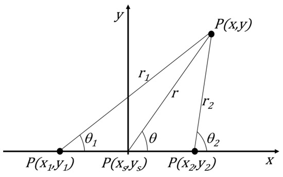
Figure 1.
Modified coordinate system based on the analytical solution of Sneddon. Reproduced with permission from [15], Elsevier, 2020.
The elastic displacements, induced by a single hydraulic fracture, in the x and y direction are (Figure 1):
where P is the internal pressure of the hydraulic fracture, v is the bulk Poisson’s ratio, and E is the bulk Young’s modulus.
The strain tensor elements are calculated by taking the partial derivative of the displacements in the x and y direction:
Directional stresses in the x and y direction are determined from the strain tensor elements (. The constitutive equation was used as the assumed boundary condition in the original Sneddon solution:
The hydrostatic pressure in the bulk rock is assumed to remain isotropic and scalar throughout the poro-elastic medium, and relates linearly to the pore pressure PP multiplied by a scaling factor α (Biot’s constant):
The pore pressure can be assumed to either be constant throughout the reservoir, for the sake of simplicity, or may spatially vary, as shown later in this study.
Combining Equation (7) with Equations (5) and (6) gives the total stress:
The shear stress is not affected by the pore pressure.
Stress tensor components () or () are used to obtain the magnitude of the principal stresses, and , for all coordinate within the observation plane by applying the standard expressions:
The maximum principal stress trajectory can be calculated with:
According to Equation (13), the principal stress trajectories are not affected by any pore pressure offsets, because the term annuls the poro-elastic terms appearing in Equations (8) and (9).
For multiple cracks, the elastic displacements, due to all the superposed hydraulic fractures, are summed directionally:
After calculating the total displacement field for multiple cracks, Equations (3)–(13) are applied to solve the strain, stress, and stress trajectories. This methodology was used to model the stress field contours resulting from two active hydraulic fractures, accounting for the effect of poro-elasticity, as shown in Figure 2.
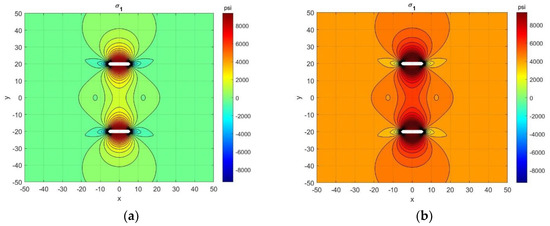
Figure 2.
Map views of virtual wellbore at x = 0, with two transverse fractures. Maximum principal stress magnitude contours (scaled in psi) for the Linear Superposition Method (LSM) model (a) with only elastic stress, and (b) with poro-elastic stress.
3.3. Static LSM Model Results
The static Linear Superposition Method (LSM) is applied here to study the spatial effect of poro-elasticity. The linear elasticity assumption and plane strain boundary condition result in a 2D displacement model and a 3D stress model. Additionally, all cracks are assumed to be cylindrical. These assumptions ensure that all 2D solutions are identical for each parallel slice in 3D space. Simulation inputs for an LSM model with two active hydraulic fractures are given in Table 1.

Table 1.
LSM model for two hydraulic fractures.
To analyze the influence of poro-elasticity on numerical displacement and stress value, the values of displacement and stress magnitudes are compared at a single coordinate (when x = 0 and y = 0) in static LSM models with Pp = 0 (Figure 2a) and Pp = 4439 (Figure 2b). Table 2 shows the numerical comparison of the principal stresses spatially. Pore pressure is shown to elevate the magnitude of the two principal stresses, at the origin of the coordinate system (x,y) = (0,0). The local pressure increase creates a stress difference as shown in Table 2, exactly equal to pore pressure (3995 psi) multiplied by Biot’s constant.
Table 2.
Principal stress magnitudes at x = 0 and y = 0.
Table 3 compares the magnitude of the principal stresses at another arbitrary point (x,y) = (10,10) to further observe the spatial effect of poro-elasticity. The principal stress magnitudes are entirely different from values previously recorded at (x,y) = (0,0). However, the results in Table 1 show that the pore pressure again increases the magnitude of both principal stresses, and the stress differences in Table 3 are exactly the same (3995 psi) as in Table 2.
Table 3.
Principal stress magnitudes at x = 10 and y = 10.
Next, assume that there exists a spatial gradient in the pore pressure, within the elastic medium of interest, with a maximum scalar gradient along the x-direction, ranging from 1000 to 4439 psi (Figure 3). Such a spatial gradient would occur in well models (map view) with a nearby legacy well at the left boundary that has depleted the reservoir pressure to 1000 psi (left boundary), while at the right hand side of the lease boundary the pristine reservoir pressure still exists (4439 psi). The local stress field will change when a horizontal child well is drilled and completed in the middle of the lease region. The contours for the spatial pore pressure, in the absence of any fractures, are shown in Figure 3.
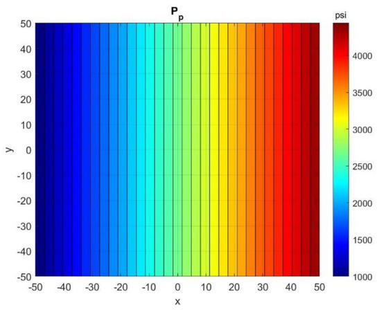
Figure 3.
Pore pressure variation in the LSM model along the lateral x-axis, ranging from 1000 to 4439 psi.
When two hydraulic fractures are introduced (Figure 2) with the condition as in Table 1, except for pore pressure varying spatially as in Figure 3, then the spatial variation in the maximum principal stress magnitude occurs, as in Figure 4. The stress contours are no longer observed to be symmetric about the wellbore at x = 0, due to the effect of variable pore pressure in the model space. In effect, the left side of Figure 4 reflects Figure 2a, and the right-hand side of Figure 4 reflects Figure 2b. Additionally, the principal stress trajectory remains symmetric for the left- and right-hand side, as shown in Figure 4b.
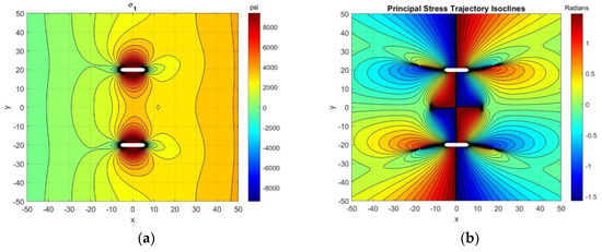
Figure 4.
LSM 2-fracture model with variable pore pressure as in Figure 3 for (a) maximum principal stress magnitude contour, and (b) principal stress trajectory isoclines.
In order to analyze the effect of variable pore pressure in the poro-elastic LSM model on the numerical displacement and stress values are compared at laterally opposite coordinate points in the model of Figure 4 (Table 4).
Table 4.
Principal stress magnitude comparison at directly opposite coordinate for variable pore pressure.
Similar to the results shown in Table 2 and Table 3, the escalation of pore pressure leads to an increase in principal stress magnitudes. The principal stress magnitude difference is exactly the same at both coordinates (−20, 20) and (20, 20). The principal stress magnitude difference spatially is observed to be uniform and constant throughout the elastic medium. Additionally, the principal stress magnitude difference between two coordinates is equal to that of the pore pressure difference of the same coordinates multiplied by the Biot’s constant:
The stress magnitudes induced into the poro-elastic medium by the hydraulic fractures are increased when the pore pressure increases. In the examples given, the stress increases in a linear fashion in every spatial direction towards higher (positive) x-coordinates. In the y-direction, the pore pressure gradient vanishes, and differential stress magnitudes are reduced everywhere along a certain y-coordinate by the same amount, equal to the local pore pressure multiplied by the Biot’s constant.
3.4. Sub-Conclusions
Several sub-conclusions can be inferred from the poro-elastic models presented in this section:
- Principal stress trajectories are not affected by the regional pore pressure variations (Figure 4b).
- However, pore pressure changes have a direct relationship with principal stress magnitudes—as pore pressure increases, the principal stress magnitudes will increase (Figure 4a).
- Changes in the principal stress magnitude, induced by the pore pressure, were constant for all spatial coordinates in the elastic medium.
- Induced changes in the principal stress magnitudes are equal to the pore pressure multiplied by the Biot’s constant.
4. Advancing TLSM with Time-Dependent Pressure
In this section, the Time-Stepped Linear Superposition Method (TLSM) is integrated with field Diagnostic Fracture Injection Test data. This integration of data into the TLSM model allows for a more realistic interpretation of the hydraulic fracturing process, accounting for the time-dependent changes in the pressure load of individual fractures.
4.1. Time-Dependent Pressure Equations and Assumptions
The present TLSM model adopts several assumptions in order to simplify the fracture propagation problem: (1) all hydraulic fractures are assumed to have the same storage capacity and propagate uniformly to contain all injection fluid, (2) linear elasticity, and (3) plane strain. The stress concentration induced by each hydraulic fracture at any point in the elastic medium can be described by the summation of the displacements in each direction. The directional strain tensor solutions are determined using a partial derivative of the spatial displacement field. Directional stress magnitudes are then calculated from these strain tensors. The maximum principal stress trajectory calculated at the fracture tip determines the direction of future fracture growth.
A simplified failure criterion is used such that if the tensile principal stress at the tip of the fracture exceeds that of the rock strength, then the fracture propagates. Conversely, when stresses at the fracture tip due to the pressure load are no longer critical, then the fracture will no longer propagate. Following mechanical failure, the propagation path of the hydraulic fracture is calculated with a Eulerian displacement scheme. The successive predicted future location zj of each fracture tip is [8,16]:
where z is the fracture tip position in 2D space, t is the time in seconds, V is the fracture velocity in ft/s, and Δt is the time step in seconds.
Using Equation (17), the fracture growth velocity (V) accounts for any changes in pump rates in the DFIT data. Additionally, the timestep parameter (Δt), is used to account for events happening in the DFIT data such as the start of injection, the duration of injection, and shut-in time.
4.2. Dynamic Fracture Propagation
TLSM models of fracture propagation use the changes in the global displacement field at each time-step to adjust the incremental superstition of successive displacement fields. Each time-step accounts for the concurrent fluid volume injected, and the elastic deformation resulting from such enacted force. Static equilibrium is assumed at each time-step, which means the sum of all forces in each direction is constrained to zero at every predetermined time-step. Additionally, no linear or angular accelerations are permitted to occur. This implies that at every successive time-step, the hydraulic fracture in equilibrium can propagate, but its linear and angular velocities remain constant. Similarly to previously used, common fracture propagation frameworks, there is no acceleration involved in the systems modeled. Thus, the inertia term in the equation of motion is neglected.
The justification for neglecting the inertia terms is that any stress perturbations involving inertia would be very small or absent in conventional dynamic simulations of fracture propagation. In other words, such approaches could be called quasi-static in the strict sense that dynamic terms are assumed to remain negligible and thus are neglected altogether. Such simplification may not be warranted, for example, if a fracture propagation case has an abrupt initiation or termination, such that dynamic stress perturbations associated with the occurrence of seismic waves may become significant. Seismicity may cause pressure fronts to run ahead of the stress-tip-induced stress perturbations, and would potentially lower the threshold for failure at the fracture tip, due to dynamically superposed stress field changes resulting from inertia effects [27].
4.3. Diagnostic Fracture Injection Tests (DFIT)
In unconventional exploration, diagnostic fracture injection tests (DFIT) have become a primary method to determine key reservoir parameters—for later use in hydraulic fracture treatment operations—such as the fluid efficiency, minimum in situ stress, pore pressure, leak-off coefficient, and fracture gradient. DFITs are typically completed in short time-frames spanning a mere couple of days, and commonly less than two weeks, which is significantly shorter as compared to the traditional pressure build-up tests, which could last several weeks due to the requirement of stable-flowing conditions, before the start of the shut-in period [28]. DFITs involve the injection of a relatively small fluid volume, typically at a first stage in the toe of a newly drilled horizontal well, with a constant injection rate to obtain information about the hydraulic fracture treatment parameters as well as the reservoir. Due to the risk of formation damage, the fluid injection rate is commonly limited to a constant rate of 5–6 bbl/min over a very brief period of 3–5 min [29].
The well is shut-in following the DFIT injection, and the pressure fall-off is recorded over several days—either at the surface or at the bottom-hole level. When the reservoir pressure is equal to or greater than the hydrostatic pressure in the wellbore, the recording of surface pressure response data suffices [30]. During the shut-in period, injection fluid gradually leaks off into the reservoir, causing the hydraulic mini-fracture created by the DFIT to close. Using the data obtained during the pressure de-escalation period, after shut-in, one can determine the fracture closure stress and pore pressure [31].
Traditionally, DFIT analysis methods use the G-function model and the tangent line method to evaluate the fracture closure stress. The G-function represents the shut-in time [32]. Recent developments in DFIT analysis apply forward models and inverse calculations to determine the stress-dependent, unpropped fracture conductivity [33].
Data from DFITs can be used to enhance the realistic representation of fracture propagation models. For example, DFIT-induced fractures in a pressure depleted environment will have a larger footprint near the depleted region [34]. Additionally, the growth of hydraulic fractures during injection and shut-in was observed to be episodic, where the fractures grow intermittently through phases instead of in a steady continuous rate [35]. The presence of any natural fractures has also been shown to influence the responses of hydraulic fractures during DFITs. The pumping schedule and the hydraulic fracture propagation path may impact the DFIT estimation of the minimum horizontal stress [36].
4.4. Field DFIT Data and Simulation Parameters
Field data from a Diagnostic Fracture Injection Test are shown in Figure 5. The breakdown pressure, instantaneous shut-in pressure (ISIP), fracture propagation pressure, fracture closure pressure, and injection cycles are labeled. During this injection cycle, the injection rate remains constant while the reservoir pressure is monitored and recorded. The TLSM model applied here assumes the existence of failure nuclei in the elastic medium and that breakdown pressure already occurred. Hence, the second injection cycle is used for hydraulic fracture propagation. The associated data with the start time of the second injection cycle normalized to 0 are shown in Figure 6.

Figure 5.
Field diagnostic fracture injection test (DFIT) pressure vs. time data for Well 3H.
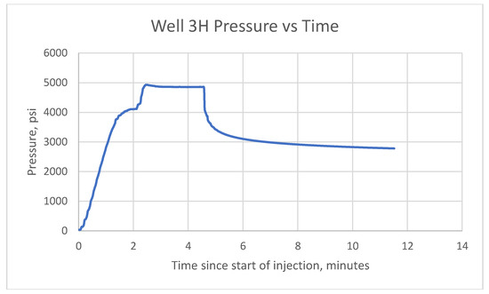
Figure 6.
Field DFIT pressure vs. time data for Well 3H at the second injection cycle.
The starting pressure recorded in the analyzed data (of Figure 5 and Figure 6) is 35.5 psia; hence, the pressure gauge is assumed to be positioned at the surface. Neglecting pipe friction, the bottom hole tubing pressure (BHTP) is calculated by:
where Ps is the recorded surface pressure of 35.5 psia and Pp is the calculated constant pore pressure of 4439 psia (assumed pore pressure gradient of 0.6 psi/ft). The bottom hole pressure vs. time curve is calculated using Equation (18) and shown in Figure 7. The fracture propagation pressure inferred from the bottom hole pressure vs. time curve in Figure 5 is 9370.83 psi and was integrated into the TLSM model. This fracture propagation pressure is constrained to be constant along with the fluid injection rate during the fracture propagation process. Further DFIT pressure and time parameters used in TLSM are given in Table 5. A typical constant injection rate of 6 bpm/min for a DFIT test was assumed to simulate the fracture propagation process due to fluid injection [29]. This allows for the calculation of total injected volume, and the number of fractures to contain those fluid volumes with assumed fracture geometry. Further fracture geometric and volumetric parameters used in TLSM are given in Table 6.
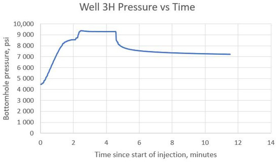
Figure 7.
Calculated bottom hole pressure vs. time for Well 3H.
Table 5.
Parameters gathered from DFIT data used for Time-Stepped Linear Superposition Method (TLSM) simulation.
Table 6.
Assumed injection and fracture volumetric parameters used in TLSM.
4.5. TLSM DFIT Model Results
Figure 8 shows the fracture pressure vs. time curve used in the TLSM model, which was set to 0 psi at time 0 to represent an undisturbed and unfractured formation. The fracture pressure was then increased to 9371 psi and remained constant for 4.58 min. At the 4.58 min mark in Figure 8, the injection cycle ends, and the hydraulic fractures cease to propagate. When hydraulic fracture propagation ceases at the end of the injection cycle, fracture pressure de-escalation begins due to leak-off.
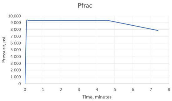
Figure 8.
Fracture pressure vs. time with end of injection at 4.58 min.
To investigate the spatial effect of induced stress by hydraulic fracturing, Figure 9 shows the maximum principal stress recorded at (x,y) = (0,0) vs. time curve with the maximum principal stress at a distance of 25 ft away from the perforations, using with the same fracture pressure inputs as in Figure 8. The maximum principal stress at (x,y) = (0,0) is observed to increase rapidly at the start of injection and peaked at approximately 11.22 s after the injection cycle begins. However, the maximum principal stress begins to decrease exponentially even before the end of injection. This decline in maximum principal stress is continued until the pore pressure is reached. The signature plot trajectory is particularly similar to that of the DFIT data, where the pressure increases dramatically as the fracture propagates, exponentially drops, and plateaus as the fracture closes.
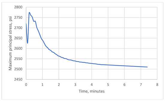
Figure 9.
Calculated maximum principal stress vs. time during the injection cycle at x = 0 and y = 0. End of injection is at 4.58 min.
4.6. Sub-Conclusions
Several sub-conclusions can be formed based on integrated DFIT data with the TLSM model in this section:
- The maximum principal stress at (x,y) = (0,0) during injection increases dramatically as the fracture propagates, exponentially drops, and steadies on a plateau value as the fracture closes, while injection pressure remained constant (Figure 9).
- Hence, the variation in maximum principal stress is primarily caused by the changes in fracture geometry as the fracture propagates, rather than by changes in injection pressure.
5. TLSM Results with Imposed Pore Pressure Gradient
In this section, the dynamic propagation of two hydraulic fractures is modeled with a regional pore pressure gradient with and without a near-field stress superposition due to a pre-existing natural fracture. While the pore pressure gradient alone does not lead to any discernable reorientation of propagating hydraulic fractures (Section 5.1), when a near-field stress perturbation exists (in this case a pressurized natural fracture, Section 5.2), such reorientation is very pervasive.
5.1. Hydraulic Fracture Propagation—Pre-Existing Pore Pressure Gradient
Figure 10a,b show, respectively, that the scalar pore pressure magnitude and stress trajectory isoclines do not exist in the initial poro-elastic medium before the onset of the hydraulic fracture treatment. The initial pore pressure varies spatially, but no stress tensor field exists (Figure 10a). The principal stress trajectory isoclines show no spatial variation and are zero everywhere, since hydraulic fractures have not yet been activated to impose a stress tensor field.
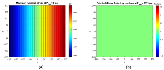
Figure 10.
Initial pre-hydraulic fracturing TLSM model results for (a) magnitude of pore pressure values (psi), and (b) no principal stress trajectory isoclines occur at t = 0 s.
Figure 11 shows the TLSM results for the first hydraulic fracture nuclei imposed on the 2D poro-elastic medium used in TLSM. The presence of the pore pressure gradient does impact the maximum principal stress magnitudes but does not affect the principal stress trajectories isoclines. The extent of the altered maximum principal stress is limited to that of the area around the hydraulic fracture, while the principal stress trajectories now appear everywhere in the poro-elastic medium due to the distortion of the scalar pressure field by the stress tensor field induced by the fractures.
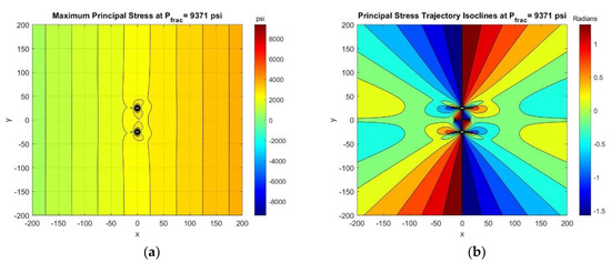
Figure 11.
TLSM model results for the initial hydraulic fracture nuclei showing (a) maximum principal stress. Color code is shifted with respect to Figure 10a, due to stress peaks at the fracture nuclei. (b) Principal stress trajectory isoclines at t = 0.093 min. TLSM results were generated in 0.466 s including post-processing.
Figure 12 shows the next successive hydraulic fracture propagation step after Figure 11. The maximum principal stress and the maximum principal stress trajectory isoclines are observed to be further changed as the fractures propagate. The maximum principal stress contours increase uniformly from the left to the right boundary of the study region, with the pressure depletion attributed to a Type B intervention (see Section 2). Alterations in the magnitude of the stress occur in the vicinity of the imposed hydraulic fractures, and the principal stress trajectories are also altered systematically throughout the medium.
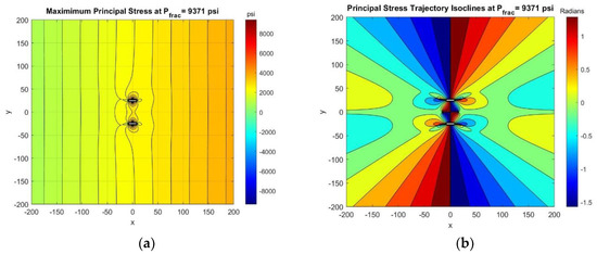
Figure 12.
TLSM model results for the second successive hydraulic fractures showing (a) maximum principal stress, and (b) principal stress trajectory isoclines at t = 1.151 min. TLSM results were generated in 1.151 s including post-processing.
Figure 13 shows the TLSM results for the final hydraulic fractures at the end of the injection period, immediately prior to the de-escalation of fracture pressure due to shut-in. The hydraulic fractures are observed to diverge uniformly through region of variable pore pressure. The stress induced by the propagated hydraulic fracture at this stage is dominant over the existing pore pressure in the reservoir.

Figure 13.
TLSM results at the end of injection showing (a) maximum principal stress, and (b) principal stress trajectory isoclines at t = 4.583 min. TLSM results were generated in 50.101 s including post-processing.
Figure 14 shows TLSM results for the hydraulic fractures at the very end of the simulation. The principal stress trajectory isoclines during leak-off remained unchanged as compared to the result at the end of injection (Figure 13). This is due to the neglection of fracture closure in the current TLSM model. In more complex scenarios, the closure of hydraulic fractures would reduce fracture width and fracture length, and thus would change the induced stress at every point in the model. Similar to the results in Figure 13, the propagated hydraulic fracture remains the dominant stress inducer relative to the existing pore pressure. As the pressure inside the fracture decreases due to leak-off, so does the maximum principal stress.
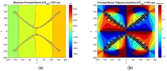
Figure 14.
TLSM results at the end of the model showing (a) maximum principal stress, and (b) principal stress trajectory isoclines at t = 7.389 min. TLSM results were generated in 26.095 min including post-processing.
Figure 11, Figure 12, Figure 13 and Figure 14 presented in this paper are snapshots of dynamic results from TLSM. Dynamic portrayals of Figure 11, Figure 12, Figure 13 and Figure 14 are given in the Supplementary Materials as Figure S1a,b. Figure S1a shows the dynamic TLSM result for two hydraulic fractures in a region with pore pressure gradient showing maximum principal stress, as shown in Figure 11a, Figure 12a, Figure 13a, Figure 14a. Figure S1b shows the dynamic TLSM result for two hydraulic fractures in a region with pore pressure gradient showing principal stress isoclines, as shown in Figure 11b, Figure 12b, Figure 13b, Figure 14b.
5.2. Hydraulic Fracture Propagation—Uniform Pressure Gradient and a Pre-Existing Near-Field Stress
In Section 5.1, the pore-pressure gradient did not appear to modify hydraulic fracture propagation direction. In this section, a pre-existing pressurized natural fracture is assumed, in addition to the pore-pressure gradient. The natural fracture was imposed at a position of x = −25 feet and y = 100 ft, with a half-length of 100 ft, and oriented −30° from the positive x-axis. The average pressure inside the fault was set to 1000 psi.
The far-field stress imposed by the natural fracture changed the propagation direction of the two hydraulic fractures. The final hydraulic fracture propagation patterns at the end of injection period are shown in Figure 15, and after leak-off shown in Figure 16. The final fracture pattern no longer resembles that of Figure 13 and Figure 14. Additionally, the hydraulic fractures propagated to develop mutual fracture hits, shown by their collision, as well as with the natural fracture. Stress reorientation induced by a near-field stress superposition due to a nearby natural fracture may profoundly affect the hydraulic fracture propagation paths. The pressure depletion due to Type B interventions may not be a primary cause for stress reorientation, but Type A interventions may run into local stress perturbations that alter the fracture path. Previous works attributed fracture reorientation and stress reversals to pore pressure changes by reservoir pressure depletion due to production [12,13]. However, pressure depletion in wells would not cause deviatoric stress changes, thus will not change the preferred fracture paths in the reservoir.
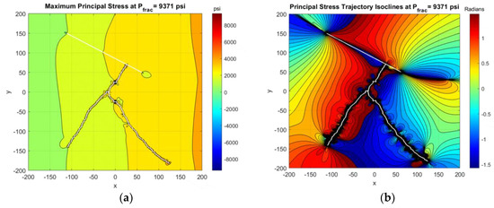
Figure 15.
TLSM results at the end of injection showing (a) maximum principal stress, and (b) principal stress trajectory isoclines at t = 4.583 min. TLSM results were generated in 53.101 s including post-processing.
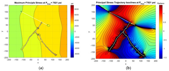
Figure 16.
TLSM results at the end of the model showing (a) maximum principal stress, and (b) principal stress trajectory isoclines at t = 7.389 min. TLSM results were generated in 26.145 min including post-processing.
Figure 15 and Figure 16 presented in this paper are snapshots of dynamic results from TLSM. Dynamic portrayals of Figure 15 and Figure 16 are given in the Supplementary Materials as Figure S2a,b. Figure S2a shows the dynamic TLSM result for two hydraulic fractures in proximity to a pressurized natural fracture showing maximum principal stress, as shown in Figure 15a, Figure 16a. Figure S2b shows the dynamic TLSM result for two hydraulic fractures in proximity to a pressurized natural fracture showing principal stress trajectory isoclines, as shown in Figure 15b, Figure 16b.
5.3. Sub-Conclusions
The model results generated by TLSM for the competing effects of poro-elasticity and far-field stress gives rise to the following sub-conclusions:
- The spatial variation of pore pressure does not affect the fracture propagation direction (Figure 13).
- Changes in stress state are concentrated in areas closest to the hydraulic fractures.
- The superposition of a near-field stress, in this case a pressurized natural fracture, causes stress reversals, as well as the reorientation of what previously would be symmetric hydraulic fracture patterns.
6. Discussion
6.1. Pore Pressure and Principal Stress Reorientation
Prior suggestions that principal stress re-orientations would occur due to pore pressure depletion [12,37] (i.e., Type B interventions) seem untenable, as follows from the model results in this study. Stress reversals are not a primary effect of gradients in pore pressure, but occur due to certain far-field and near-field stress superposition situations.
In practice, local changes in near-field stress can be induced by Type A interventions when a nearby, new child well is hydraulically pressured [38], which then causes a deviatoric stress field to arise in the vicinity of the well. Alternatively, a pre-existing natural fracture may also cause a change in the so-called near-field stress. The reorientation of hydraulic fractures observed in high and low pore pressure areas may not be an artifact of spatial variation of pore pressure, but is instead due to spatial variations of the shadowed stresses.
6.2. Strengths and Weaknesses
Similar to other hydraulic fracture propagation modeling methods, there are strengths and weaknesses associated with the use of TLSM. Among the strengths of TLSM are that it offers grid-less, closed-form, semi-analytical solutions for non-planar fracture propagation. By avoiding adaptive grid-refinement, fast simulation of multiple competitive hydraulic fracture propagation and infinite resolution are achieved. Among the weaknesses of both LSM and TLSM is that the current codes are constrained to a linear elasticity assumption.
The present study adapted the code to account for linear poro-elasticity and also accommodates field-based pressure inputs (DFIT). The growth of hydraulic fractures is constrained to account for all the fluid volumes injected at each timestep. Hence, the hydraulic fractures must propagate in order to contain the volumes injected. Since all hydraulic fractures are assumed to have the same storage capacity and a positive propagation velocity, fracture closure and the reduction in hydraulic fracture length were neglected.
6.3. Future Work
This study focused on the modeling of fracture propagation with TLSM, assuming internally pressurized fractures with the same storage capacity to accommodate all injection fluid. Due to fracture closure during leak-off, reduction in the conductive length of the hydraulic fracture occurs [38]. Instead of the current constant volume injection scheme used in the current code, a volume-dependent fracture geometry scheme may be implemented. In future studies, the TLSM code can be modified to account for injection volume-dependent fracture propagation of each fracture. The fluid leak-off process can be modeled by coupling the TLSM fracture propagation simulator with our semi-analytical simulator for fluid flow in fractured porous media based on Complex Analysis Methods (CAM). Key algorithms and fundamental theory for both TLSM and CAM were previously published in leading applied mathematics journals [15,39,40].
7. Conclusions
Real world DFIT data were used in TLSM to model and observe the effect of time-dependent pressure and poro-elasticity on the development of the hydraulic fracture networks. The effects of time-dependent pressure and poro-elasticity were analyzed in the TLSM results presented. The conclusions are valid for the specific parameters considered in this study—supported by the dynamic visualizations of the changes in spatial stress concentrations during the time-dependent pressure hydraulic fracturing process.
We conclude, regarding spatial pore pressure variations and fracture propagation, the following:
- Principal stress trajectories were not affected by the regional pore pressure variations (Figure 4b).
- However, pore pressure changes have a direct relationship with principal stress magnitudes—as pore pressure increases, the principal stress magnitudes will increase (Figure 4a)
- Induced changes in the principal stress magnitudes were equal to the pore pressure multiplied by the Biot’s constant.
From the integration of DFIT field data in our and TLSM models, we conclude:
- The maximum principal stress at (x,y) = (0,0) during injection increases dramatically as the fracture propagates, and the principal stress magnitude exponentially first drops, and then plateaus as the fracture closes, while injection pressure remained constant (Figure 9).
- Hence, the variations in the maximum principal stress are primarily caused by the changes in fracture geometry as the fracture propagates, rather than changes in injection pressure.
Regarding the effects of poro-elasticity and near-field stress changes, we conclude:
- Changes in stress state are concentrated in areas closest to the hydraulic fractures (Figure 13).
- The superposition of a near-field stress, in this case a pressurized natural fracture, caused stress reversals, as well as the reorientation of what previously would be symmetric hydraulic fracture patterns (Figure 15).
- For all cases, pore pressure effects related to Type B well interventions do not seem to be a primary driver of stress reorientation in the reservoir.
- Instead of pore pressure, the stress reorientation in the reservoir can be attributed to a change in imposed near-field stresses related to Type A well interventions.
Supplementary Materials
The following are available online at https://www.mdpi.com/1996-1073/13/24/6474/s1, Figure S1a: Dynamic TLSM result for two hydraulic fractures in a region with pore pressure gradient showing maximum principal stress, as shown in Figure 11a, Figure 12a, Figure 13a, Figure 14a. Figure S1b: Dynamic TLSM result for two hydraulic fractures in a region with pore pressure gradient showing principal stress isoclines, as shown in Figure 11b, Figure 12b, Figure 13b, Figure 14b. Figure S2a: Dynamic TLSM result for two hydraulic fractures in proximity to a pressurized natural fracture showing maximum principal stress, as shown in Figure 15a, Figure 16a. Figure S2b: Dynamic TLSM result for two hydraulic fractures in proximity to a pressurized natural fracture showing principal stress trajectory isoclines, as shown in Figure 15b, Figure 16b.
Author Contributions
Conceptualization, R.W.; methodology, T.P. and R.W.; software, T.P. and R.W.; investigation, T.P.; writing-original draft preparation, T.P. and R.W.; writing-review and editing, T.P. and R.W.; supervision, R.W.; funding acquisition, R.W. Both authors have read and agreed to the published version of the manuscript.
Funding
This project was sponsored by the Crisman-Berg Hughes consortium and startup funds from the Texas A&M Engineering Experiment Station (TEES).
Conflicts of Interest
The authors declare no conflict of interest.
References
- Masouleh, S.F.; Kumar, D.; Ghassemi, A. Three-Dimensional Geomechanical Modeling and Analysis of Refracturing and “Frac-Hits” in Unconventional Reservoirs. Energies 2020, 13, 5352. [Google Scholar] [CrossRef]
- Pei, Y.; Wang, J.; Yu, W.; Sepehrnoori, K. Investigation of Lateral Fracture Complexity to Mitigate Frac Hits During Interwell Fracturing. In Proceedings of the 8th Unconventional Resources Technology Conference Virtual, Austin, TX, USA, 20–22 July 2020. [Google Scholar]
- Ciezobka, J.; Courtier, J.; Wicker, J. Hydraulic Fracturing Test Site (HFTS)—Project Overview and Summary of Results. In Proceedings of the 6th Unconventional Resources Technology Conference, Houston, TX, USA, 23–25 July 2018. [Google Scholar]
- Raterman, K.; Farrell, H.; Mora, O.; Janssen, A.; Gomez, G.; Busetti, S.; Warren, M. Sampling a stimulated rock volume: An eagle ford example. In Proceedings of the 6th Unconventional Resources Technology Conference, Austin, TX, USA, 24–26 July 2018. [Google Scholar]
- Raterman, K.; Liu, Y.; Warren, L. Analysis of a Drained Rock Volume: An Eagle Ford Example. In Proceedings of the 7th Unconventional Resources Technology Conference, Denver, CO, USA, 22–24 July 2019. [Google Scholar]
- Stegent, N.; Candler, C. Downhole Microseismic Mapping of More Than 400 Fracturing Stages on a Multiwell Pad at the Hydraulic Fracturing Test Site (HFTS): Discussion of Operational Challenges and Analytic Results. In Proceedings of the 6th Unconventional Resources Technology Conference, Houston, TX, USA, 23–25 July 2018. [Google Scholar]
- Stegent, N.; Dusterhoft, R.; Menon, H. Insight into Hydraulic Fracture Geometries Using Fracture Modeling Honoring Field Data Measurements and Post-Fracture Production. In Proceedings of the SPE Europec Featured at 81st EAGE Conference and Exhibition, London, UK, 3–6 June 2019. [Google Scholar]
- Weijermars, R.; Pham, T.; Stegent, N.; Dusterhoft, R. Hydraulic fracture propagation paths modeled using time-stepped linear superposition method (TSLM): Application to fracture treatment stages with interacting hydraulic and natural fractures at the Wolfcamp Field Test Site (HFTS). In Proceedings of the 54th US Rock Mechanics/Geomechanics Virtual, Golden, CO, USA, 28 June–1 July 2020. [Google Scholar]
- Sesetty, V.; Ghassemi, A. Simulation and analysis of fracture swarms observed in the Eagle Ford Field experiment. In Proceedings of the SPE Hydraulic Fracturing Technology Conference and Exhibition, The Woodlands, TX, USA, 5–7 February 2019. [Google Scholar]
- Weijers, L.; Pater, C.J. Fracture Reorientation in Model Tests. In Proceedings of the SPE Formation Damage Control Symposium, Lafayette, LA, USA, 26–27 February 1992. [Google Scholar]
- Wright, C.A. Reorientation of Propped Refracture Treatments in the Lost Hills Field. In Proceedings of the SPE Western Regional Meeting, Long Beach, CA, USA, 23–25 March 1994. [Google Scholar]
- Bruno, M.S.; Nakagawa, F.M. Pore Pressure Influence on Tensile Fracture Propagation in Sedimentary Rock. Int. J. Rock Mech. 1991, 28, 251–273. [Google Scholar] [CrossRef]
- Agrawal, S.; Sharma, M.M. Impact of Pore Pressure Depletion on Stress Reorientation and Its Implications on the Growth of Child Well Fractures. In Proceedings of the 6th Unconventional Resources Technology Conference, Houston, TX, USA, 23–25 July 2018. [Google Scholar]
- Wright, C.A.; Conant, R.A. Hydraulic Fracture Reorientation in Primary and Secondary Recovery from Low-Permeability Reservoirs. In Proceedings of the SPE Annual Technical Conference and Exhibition, Dallas, TX, USA, 22–25 October 1995. [Google Scholar]
- Pham, T.; Weijermars, R. Solving Stress Tensor Fields around Multiple Pressure-Loaded Fractures using a Linear Superposition Method (LSM). Appl. Math. Model. 2020, 88, 418–436. [Google Scholar] [CrossRef]
- Pham, T.; Weijermars, R. Development of Hydraulic Fracture Hits and Fracture Redirection Visualized for Consecutive Fracture Stages with Fast Time-stepped Linear Superposition Method (TLSM). In Proceedings of the Unconventional Resources Technology Conference Virtual, Golden, CO, USA, 20–22 July 2020. [Google Scholar]
- Weijermars, R.; Wang, J.; Pham, T. Borehole Failure Mechanisms in Naturally and Hydraulically Fractured Formations Investigated with a Fast Time-stepped Linear Superposition Method (TLSM). In Proceedings of the 54th US Rock Mechanics/Geomechanics Symposium Virtual, Austin, TX, USA, 28 June–1 July 2020. [Google Scholar]
- Zhai, Z.; Sharma, M.M. Estimating Fracture Reorientation due to Long Term Fluid Injection/Production. In Proceedings of the Production and Operations Symposium, Oklahoma City, OK, USA, 31 March–3 April 2007. [Google Scholar]
- Elbel, J.L.; Mack, M.G. Refracturing: Observations and Theories. In Proceedings of the SPE Production Operations Symposium, Oklahoma City, OK, USA, 21–23 March 1993. [Google Scholar]
- Weijermars, R.; Zhang, X.; Schultz-Ela, D. Geomechanics of fracture caging in wellbores. Geo. J. Int. 2013, 193, 1119–1132. [Google Scholar] [CrossRef]
- Weijermars, R. Stress Cages and Fracture Cages in Stress Trajectory Models of Wellbores: Implications for Pressure Management During Drilling and Hydraulic Fracturing. J. Nat. Gas Sci. Eng. 2016, 36, 986–1003. [Google Scholar] [CrossRef]
- Thomas, N.; Weijermars, R. Comprehensive Atlas of Stress Trajectory Patterns and Stress Magnitudes Around Cylindrical Holes in Rock Bodies for Geoscientific and Geotechnical Applications. Earth Sci. Rev. 2018, 179, 303–371. [Google Scholar] [CrossRef]
- Weijermars, R.; Wang, J.; Nelson, R. Stress concentrations and failure modes in horizontal wells accounting for elastic anisotropy of shale formations. Earth Sci. Rev. 2020, 200, 102957. [Google Scholar] [CrossRef]
- Gao, Q.; Ghassemi, A. Pore Pressure and Stress Distributions Around a Hydraulic Fracture in Heterogeneous Rock. Rock Mech. Rock Eng. 2017, 50, 3157–3173. [Google Scholar] [CrossRef]
- Hidayati, D.T.; Chen, H.Y.; Teufel, L.W. Flow-Induced Stress Reorientation in a Multiple-Well Reservoir. In Proceedings of the SPE Rocky Mountain Petroleum Technology Conference, Keystone, CO, USA, 21–23 May 2001. [Google Scholar]
- Weijermars, R.; Pham, T.; Ettehad, M. Linear Superposition Method (LSM) for Solving Stress Tensor Fields and Displacement Vector Fields: Application to Multiple Pressure-Loaded Circular Holes in an Elastic Plate with Far-Field Stress. Appl. Math. Comput. 2020, 381, 125234. [Google Scholar] [CrossRef]
- Zhuang, Z.; Liu, Z.; Cheng, B.; Liao, J. Extended Finite Element Method; Computational Mechanics Series; Tsinghua University Press: Beijing, China, 2014. [Google Scholar]
- Wallace, J.; Kabir, C.S.; Cipolla, C. Multiphysics Investigation of Diagnostic Fracture Injection Tests in Unconventional Reservoirs. In Proceedings of the SPE Hydraulic Fracturing Technology Conference, The Woodlands, TX, USA, 4–6 February 2014. [Google Scholar]
- Barree, R.D.; Miskimins, J.L.; Gilbert, J.V. Diagnostic Fracture Injection Tests: Common Mistakes Misfires, and Misdiagnoses. In Proceedings of the SPE Western North American and Rocky Mountain Join Regional Meeting, Denver, CO, USA, 16–18 April 2014. [Google Scholar]
- Hawkes, R.V.; Bachman, R.; Nicholson, K.; Cramer, D.D.; Chipperfield, S.T. Good Tests Cost Money, Bad Tests Cost More—A Critical Review of DFIT and Analysis Gone Wrong. In Proceedings of the SPE International Hydraulic Fracturing Technology Conference and Exhibition, Muscat, Oman, 16–18 October 2018. [Google Scholar]
- Zheng, S.; Manchanda, R.; Wang, H.; Sharma, M. DFIT Analysis and Interpretation in Layered Rocks. In Proceedings of the SPE Hydraulic Fracturing Technology Conference and Exhibition, The Woodlands, TX, USA, 4–6 February 2020. [Google Scholar]
- Nolte, K.G.; Maniere, J.L.; Owens, K.A. After-Closure Analysis of Fracture Calibration Tests. In Proceedings of the SPE Annual Technical Conference and Exhibition, San Antonio, TX, USA, 5–8 October 1997. [Google Scholar]
- Wang, H.; Sharma, M.M. Estimating Unpropped Fracture Conductivity and Compliance from Diagnostic Fracture Injection Tests. In Proceedings of the SPE Hydraulic Fracturing Technology Conference and Exhibition, The Woodlands, TX, USA, 23–25 January 2018. [Google Scholar]
- Zheng, S.; Manchanda, R.; Wang, H.; Sharma, M. Fully 3-D Simulation of Diagnostic Fracture Injection Tests with Application in Depleted Reservoirs. In Proceedings of the Unconventional Resources Technology Conference, Denver, CO, USA, 22–24 July 2019. [Google Scholar]
- Zanganeh, B.; MacKay, M.K.; Clarkson, C.R.; Jones, J.R. DFIT Analysis in Low Leakoff Formations: A Duvernay Case Study. In Proceedings of the SPE Canada Unconventional Resources Conference, Calgary, AB, Canada, 13–14 March 2018. [Google Scholar]
- Kamali, A.; Ghassemi, A. DFIT Considering Complex Interactions of Hydraulic and Natural Fractures. In Proceedings of the SPE Hydraulic Fracturing Technology Conference and Exhibition, The Woodlands, TX, USA, 5–7 February 2019. [Google Scholar]
- Prabhakaran, R.; Pater, H.; Shaoul, J. Pore Pressure Effects on Fracture Net Pressure and Hydraulic Fracture Containment: Insights from an Empirical and Simulation Approach. J. Pet. Sci. Eng. 2017, 157, 724–736. [Google Scholar] [CrossRef]
- Morales, R.H. An Interesting Look at Multiple Fractures: Stress Shadowing and Propagation. In Proceedings of the SPE Hydraulic Fracturing Technology Conference and Exhibition, The Woodlands, TX, USA, 4–6 February 2020. [Google Scholar]
- Harmelen, A.; Weijermars, R. Complex analytical solutions for flow in hydraulically fractured hydrocarbon reservoirs with and without natural fractures. App. Math. Model. 2018, 56, 137–157. [Google Scholar] [CrossRef]
- Weijermars, R.; Ettehad, M. Displacement field potentials for deformation in elastic media: Theory and application to pressure-loaded boreholes. App. Math. Comput. 2019, 340, 276–295. [Google Scholar] [CrossRef]


Publisher’s Note: MDPI stays neutral with regard to jurisdictional claims in published maps and institutional affiliations. |
© 2020 by the authors. Licensee MDPI, Basel, Switzerland. This article is an open access article distributed under the terms and conditions of the Creative Commons Attribution (CC BY) license (http://creativecommons.org/licenses/by/4.0/).