Article

Surrogate Models for Wind Turbine Electrical Power and Fatigue Loads in Wind Farm

Department of Wind Energy, Technical University of Denmark, 4000 Roskilde, Denmark
*
Author to whom correspondence should be addressed.
Energies 2020, 13(23), 6360; https://doi.org/10.3390/en13236360
Submission received: 26 October 2020 / Revised: 17 November 2020 / Accepted: 26 November 2020 / Published: 2 December 2020
(This article belongs to the Special Issue Wind Farm Control Systems: Concepts and Structures)

Abstract

:
Fatigue damage of turbine components is typically computed by running a rain-flow counting algorithm on the load signals of the components. This process is not linear and time consuming, thus, it is non-trivial for an application of wind farm control design and optimisation. To compensate this limitation, this paper will develop and compare different types of surrogate models that can predict the short term damage equivalent loads and electrical power of wind turbines, with respect to various wind conditions and down regulation set-points, in a wind farm. More specifically, Linear Regression, Artificial Neural Network and Gaussian Process Regression are the types of the developed surrogate models in this work. The results showed that Gaussian Process Regression outperforms the other types of surrogate models and can effectively estimate the aforementioned target variables.

1. Introduction

In a wind farm, wind turbines are typically positioned closely together to ensure several economic benefits such as reductions in the deployment, operation and maintenance cost. However, in a row of wind turbines, the upstream turbines extract the largest amount of energy from the wind, create velocity deficits and add more turbulence to the flow for the downstream turbines. This region of flow is known as wake. The reduction in wind speeds and added turbulence in a wake will cause the downstream turbine to produce less power and accelerate the structural damage. Thus, a number of wind farm control strategies has been proposed in the literature.
A substantial amount of studies investigated the possibility to increase the aggregated wind farm power output by manipulating the wake behaviour (see [1]). These methods are mostly relevant for wind farms in low wind speeds and can be classified into two distinct classes: induction control and wake steering control. In induction control (e.g., [2,3,4]), the upstream turbines are down-regulated to reduce the thrust coefficient, aiming to reduce the velocity deficits and create a faster recovery of the wake. In wake steering (e.g., [5,6]), the upstream turbine rotor is misaligned with the ambient wind direction, with the purpose to steer the wake away from the downstream turbine. In contrast to methods increasing the power output, some works (e.g., [7,8,9]) focused on developing methods to optimise the load situation among turbines in a wind farm, which are mostly relevant for wind farms in above-rated wind conditions. Several works investigated the fatigue loads impact of turbines operating in down-regulations (e.g., [10,11,12]).
One of the key concerns in wind farm control is the turbine fatigue loads. Calculation of turbine loads, including turbine wake, typically requires Computational Fluid Dynamics (CFD) and aero-servo-elastic turbine simulations that are computationally expensive. Thus, development of a simplified and control-oriented surrogate model is motivated, which offers fast prediction of electrical power and fatigue loads in a wind farm for given control set-point of turbines.
One of the early models was developed by Frandsen [13], that maps the wake effects to an equivalent ambient turbulence. This equivalent ambient turbulence should cause the same level of fatigue load accumulation as the actual wake-induced turbulence and deficit. The Frandsen [13] approach is widely popular because of its simplicity; however, some studies (e.g., [14]) pointed out that the methods provided a conservative load result. Later, a more advanced engineering model [15], the Dynamic Wake Meandering (DWM) model, was developed. The model considers the wake velocity deficit, meandering dynamics and added wake turbulence. This model is accurate at predicting the wake-induced loads and has been validated in a number of studies (e.g., [16]). However, aero-servo-elastic turbine simulations with the DWM model are still not sufficiently fast enough for control-oriented purposes. In recent years, some simpler surrogate load models consider the various atmospheric conditions such as wind speeds, turbulence intensities and wake properties. For example, a model developed by Dimitrov [17] maps the wake properties into turbine loads, while a study by Mendez Reyes et al. [18] developed a load surrogate model that describes the turbine fatigue loads in terms of changes in yaw and wind inflow conditions. A recent study by Galinos et al. [19] considered different down-regulation power set-points in their load surrogate models.
Of the many existing works, training load surrogate models requires a substantial amount of turbine data. However, the required amount of data set of turbine loads might not always be available. Therefore, the aim of this work is to define and demonstrate a simple procedure that maps the outputs of the short-term damage equivalent loads and electrical power of a wind turbine in a wind farm, in computationally efficient surrogate models approximations. More importantly, the surrogate model developed in this work requires a small size of data set with fewer than a thousand samples. Specifically, we investigate three regression methods and identify which methods offer the best and reliable performance based on a small data set. The presented methods are Linear Regression (LR), Artificial Neural Network (ANN) and Gaussian Process Regression (GPR). In addition, this work further investigates the link between the sample size and the accuracy of surrogate models. The proposed surrogate model produces accurate and fast turbine power and load predictions in a wind farm, which is particularly useful for wind industry with a limited amount of measurement data to develop wind farm control strategy.
The remainder of this paper is organised as follows. In Section 2, we present the procedure of collecting the training data. Section 3 discusses three regression methods that are used in this study. In Section 4, evaluation of model preference and discussions are presented. Finally, it is followed by conclusions in Section 5.

2. Definition of the Surrogate Load Modeling Procedure

To acquire the input data set of this work, DTU 10MW reference turbine [20] and a high fidelity aero-elastic simulation code HAWC2 [21] were used. HAWC2 simulates wind turbines with large and flexible blades in time domain. It handles non-linear structure dynamic with arbitrary large rotation. The aerodynamic part of the code is based on the Blade Element Momentum (BEM) theory [22], but extended from the classic approach to handle dynamic inflow, dynamic stall, skew inflow, shear effects on the induction and effects from large deflections. The DWM model, which is a medium-fidelity model providing detailed information of the non-stationary inflow wind field to each individual wind turbine within a wind farm, is implemented in HAWC2 for performing wind farm simulation. Three different wind classes, namely IA, IB and IC representing different turbulence intensity reference values ( I ref ) of 0.16, 0.14 and 0.12, were used in the simulation. The mean wind speed range ( U ¯ ) was from 4 m/s to 24 m/s in 2 m/s increments, and six random turbulent seeds were used per wind speed. The simulation time was 600 seconds using time step of 0.01 s. This simulation time of 600 s is sufficiently long enough for the wake of the upwind turbine to hit the downwind turbine in the second row. The down-regulation method based on minimizing the Thrust Coefficient ( C T ) [23] was used. The down-regulation level ( δ d ) is defined as the ratio between the power demanded to generate in derating operation ( P derated ) and rated power ( P rated ):
δ d = P derated P rated
For the upstream turbine (WT-1), the down-regulation level in percentage were set as 60%, 70%, 80%, 90%, 100%. For the downstream wind turbine (WT-2) the down regulation levels were 70%, 80%, 90%, 100% for each down regulation levels of WT-1. The wind turbines in both rows were combined with all three wind classes. The Wohler exponent values (m) of 3, 4 and 10 were chosen for the bearings (yaw and shaft), the tower and the blades respectively. The space distance between the first and the second row of the wind turbines was chosen four rotor diameters (4D). This spacing represented a compromise between compactness, which minimises capital cost, and the need for adequate separations to reduce energy loss through the wind shadowing from upstream wind turbines. The ambient wind direction was set to zero degrees, which means yaw misalignment was not considered.
The results from the simulations were post-processed. The short term damage equivalent load S eq , ST for each time-series was computed using the rain-flow counting method [24]. Subsequently, the average short term Damage Equivalent Load (DEL) was computed as follows
S ¯ eq , ST = i p i · S eq , ST m 1 m
where p i = 1 6 represents the identical weight for six turbulent seeds, m is the Wohler exponent value mentioned above. For each wind speed the short-term DELs for each turbulent seed S eq , ST were combined as shown in (2) into the average short-term DEL S ¯ eq , ST corresponded to each wind speed.
The input data set D in : = { U ¯ , I ref , δ d , up , δ d , down } consists of four features. The features are: wind speed ( U ¯ ), turbulence intensity reference ( I ref ), down regulation level of the upstream and downstream wind turbine ( δ d , up and δ d , down ). The wind speed and turbulence intensity reference features consist of values that were previously described. The other two features consist of values of down regulation levels. In cases when only the loads and power of one single turbine are of interest, the power set-point for the upstream turbine is set to be 0. For example, if there was only an upstream wind turbine down regulated at 80%, then the power set-point of upstream wind turbine had to be set to 0 and the power set-point of downstream wind turbine to 0.8. In this way an extra feature addition that shows if the wind turbine is upstream or downstream, was avoided.
In Table 1 the different input values are presented. First, we have turbulent wind cases with 11 different wind speeds and three turbulent classes. For one single turbine case, the upstream turbine is operated at 60%, 70%, 80%, 90% and 100% of the rated power, that provides five variations. In a case of two turbines, five variations are for the upstream turbine and four variations are for the downstream turbine. Therefore, the total number of DEL sets that were calculated from post processing is 825 for each load channels. For the electrical power, the number of post processed results is the same since the six turbulent seeds for each wind speed were combined and the mean value was taken. The input data was a matrix of 825 × 4 elements. A general schematic diagram that represents the components of the training process is given in Figure 1.

3. Methodology

3.1. Linear Regression

In this supervised learning task, a training set is given, comprised of N observations D ob : = { X , y } , where X = [ x 1 , x 2 , , x N ] T R N × p represents the input data set and y = [ y 1 , y 2 , , y N ] T R N is denoted as the output data. The input vector x i R p has p elements of input. The goal is to predict new y i from input data x i . In Linear Regression, the predicted output y ^ i is formulated as follows.
y ^ i ( x , w ) = w 0 + w 1 x i , 1 + + w p x i , p
where w = [ w 0 , w 1 , , w p ] T R p is a vector of tunable coefficients and x i = [ x i , 1 , , x i , p ] are the input features. Learning then consists of selecting the parameters w based on the training data X and y.
In this work, the input data X is the variables listed in Table 1. With respect to the output data, for the short-term DELs surrogate model, y is the short-term DELs for each load channels. For the electrical power surrogate model, the output data y is the electrical power. A standardization was made in the data set. A 10-fold cross-validation was used and the data was divided in 90% training and 10% test set for each fold.
To predict the target variables y ^ , sklearn.linear.model.LinearRegression package in high-level programming language Python was used [25]. This model uses Ordinary Least Squares method by fitting a linear model with coefficients w to minimise the residual sum of squares between the observed targets in the data set, and the targets predicted by the linear approximation. To find the tunable coefficients w in (3), the optimisation problem is formulated as follows.
w ^ = min w | | y X w | | 2
The estimation of the coefficients for Ordinary Least Squares relies on the independence of the features. For each fold, the model was trained and the least squares optimisation (4) was computed using the singular value decomposition of X. To avoid developing an over-fitting model, a general technique for controlling model complexity known as regularization was considered. The type of regularization that was considered is commonly referred to as L 2 regularization, and the resulting model is commonly called Ridge regression [25]. For the purpose of this study, the regularization constant was tweaked in an internal cross validation. With this internal cross validation the best regularization term is chosen for each outer fold.

3.2. Artificial Neural Networks

Artificial Neural Networks (ANNs) consist of a net of various connected information processing units, so-called artificial neurons. For the purpose of this work, a feed-forward network was created. First, the input vector x = [ x 1 , x 2 , x p ] is presented to the input layer in a way that neuron i in the input layer is given an activation equal to x i . The activation is then propagated to one or several hidden layers and eventually to the output layer consisting of neurons corresponding to the components of the output vector. An example of an ANN can be seen in Figure 2.
A more general form of Equation (3) can be written as:
y ^ = x ˜ T w , x ˜ = [ 1 x 1 x 2 x p ] T
The various-weights of the model can be defined as: W ( 1 ) = [ w 1 ( 1 ) w 2 ( 1 ) w H ( 1 ) ] and W ( 2 ) = [ w 1 ( 2 ) w 2 ( 2 ) w D ( 2 ) ] , where D is the number of output neurons. By having a nonlinear activation h ( 1 ) and a number of H hidden neurons the activation of the kth output neuron can be written as:
y ^ k ( x , w ) = h ( 2 ) j = 1 H W k , j ( 2 ) h ( 1 ) x ˜ T w j ( 1 )
where h ( 1 ) is the activation function for the hidden layer, h ( 2 ) is the final transfer function for the output neuron.
For the purpose of this study, the open source machine learning library based on the Torch library PyTorch [26] was used. The Hyperbolic Tangent function was selected as the activation function and a linear function as the final transfer function for the output layer. A standardization was made in the data set. For each fold, the validation data is divided in 90% training data and 10% test data. Since the data set has a limited number of samples, this division of the data set may play a vital role to the behaviour of the model. After dividing the data, the model is trained using back-propagation and then the performance of the model is tested in each fold. The Stochastic Gradient Descent was selected as the optimizer with an early stop when the learning curve was converged. The learning rate was set to be 0.005. Two replicates of the model for each fold were created in order to train the model with the minimum loss and different starting point of backward pass. For selecting the optimal network architecture an inner loop was added to the 10-fold cross validation. Inside the loop, networks with one or two hidden layers and one to twenty neurons in each layer were trained and tested. The model with ten neurons and one hidden layer was selected as the model with the best performance and a weight decay (L2 equivalent) regularisation was implemented in order to reduce the error and prevent over-fitting [26].

3.3. Gaussian Process Regression

A Gaussian process is a random process in which any point x R d is assigned a random variable f ( x ) and the joint distribution of a finite number of these variables p ( f ( x 1 ) , , f ( x N ) ) is itself Gaussian:
p ( f | X ) = N ( f | μ , K )
where f = ( f ( x 1 ) , , f ( x N ) ) is a vector of function values of random variable x, μ = ( m ( x 1 ) , , m ( x N ) ) is a vector of mean values of random variable x and K = K i j = κ ( x i , x j ) is a positive definite kernel function or covariance function [27,28]. Given these points, a Gaussian process is a distribution over functions whose shape is defined by a positive definite kernel function or covariance function K. In general terms, a kernel or covariance function specifies the statistical relationship between two points x i , x j in the input space; that is, how distinctly a change in the value of the Gaussian process at x i correlates with a change in the Gaussian process at x j . If points x i and x j are considered to be similar by the kernel or covariance, the function values at these points, f ( x i ) and f ( x j ) , can be expected to be similar too.
In this work, since the short-term DELs for all the load channels and electrical power output are expected to be smooth, the squared exponential kernel, also known as Gaussian kernel or Radial Basis Function (RBF) kernel was used:
K = K i j = κ ( x i , x j ) = σ 2 e 1 2 l 2 ( x i x j ) T ( x i x j )
where the length parameter l controls the smoothness of the function and σ determines the average distance of the function away from its mean. This kernel function is infinitely differentiable, which means that the Gaussian process with this kernel function has mean square derivatives of all orders, and is thus very smooth [28].
A Gaussian process prior p ( f | X ) can be transformed into a Gaussian process posterior p ( f | X , y ) by including some observed data y. The posterior can then be used to make predictions f * given new input data X * :
p ( f * | X * , X , y ) = N ( f * | μ * , Σ * )
μ * = K * T K y 1 y
Σ * = K * * K * T K y 1 K *
where K y = κ ( X , X ) + σ n 2 I , K * = κ ( X , X * ) , K * * = κ ( X * , X * ) and σ n 2 is the noise term in the diagonal of K y . This term is set to zero if training targets are noise-free and to a value greater than zero if observations are noisy.
The implementation of the Gaussian Process Regression was made with the help of Python package named sklearn.gaussian_process.GaussianProcessRegressor [25] that is developed based on [28]. In this case, a standardization was not made in the data set. Again, 10-fold cross-validation was used and the data was divided in 90% training and 10% test set for each fold. The noise level was taken relatively small σ n 2 = 10 10 . Furthermore, the default optimiser was used and the number of restarts of the optimiser for finding the kernel’s parameters which maximise the log-marginal likelihood, was set to two [25].
In order to test the robustness of Gaussian Process Regression model, the performance of the model was evaluated using different number of input data sets by excluding some sample points randomly. The different input data sets consisted 742, 660, 577, 495 and 412 sample points, the results are discussed in Section 4.3.

4. Results and Discussion

4.1. Model Comparison

A quantitative comparison is carried out by computing the Normalized-Root-Mean-Square Error NRMSE:
NRMSE = i = 1 N k ( y ^ i y i ) 2 N k E ( y )
where N k is the number of observations, y ^ i is the prediction variable, y i is the observed variable and E ( y ) is the expected value of the observation variables y.
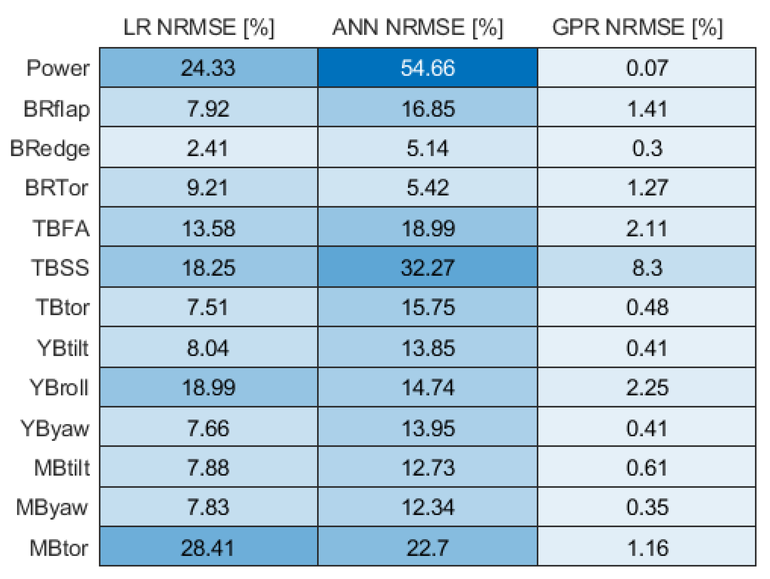
In Figure 3, the NRMSEs for all predicted variables for all models are presented. The load channels that were used are: blade root flapwise (BRflap), blade root edgewise (BRedge), blade root torsional (BRtor), tower bottom fore-aft (TBFA), tower bottom side-side (TBSS), tower bottom torsional (TBtor), yaw bearing tilt (YBtilt), yaw bearing roll (YBroll), yaw bearing yaw (YByaw), main bearing tilt (MBtilt), main bearing yaw (MByaw) and main bearing torsional (MBtor) moments. In addition to the loads, the prediction of electrical power (Power) is also of interest in this work.
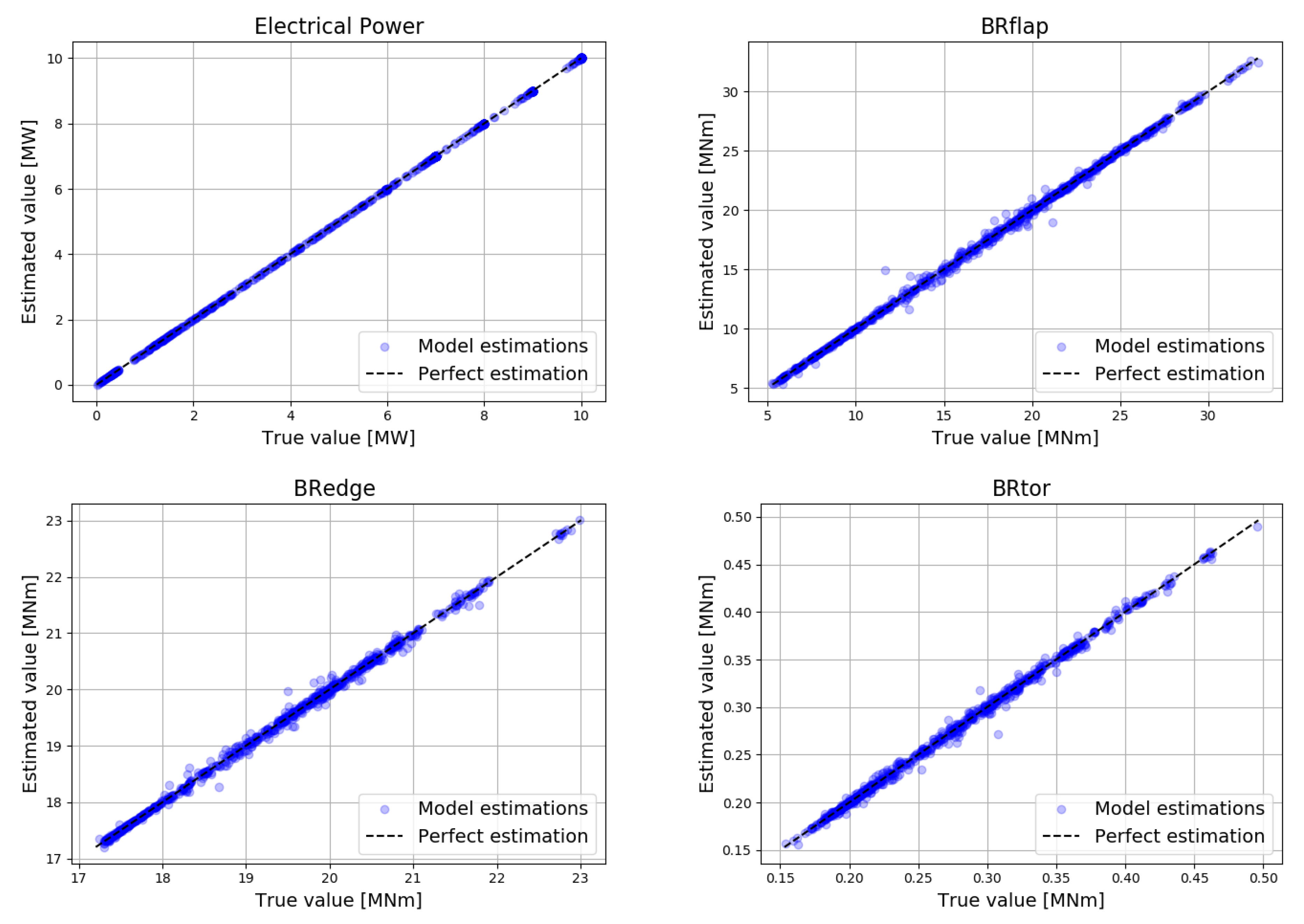
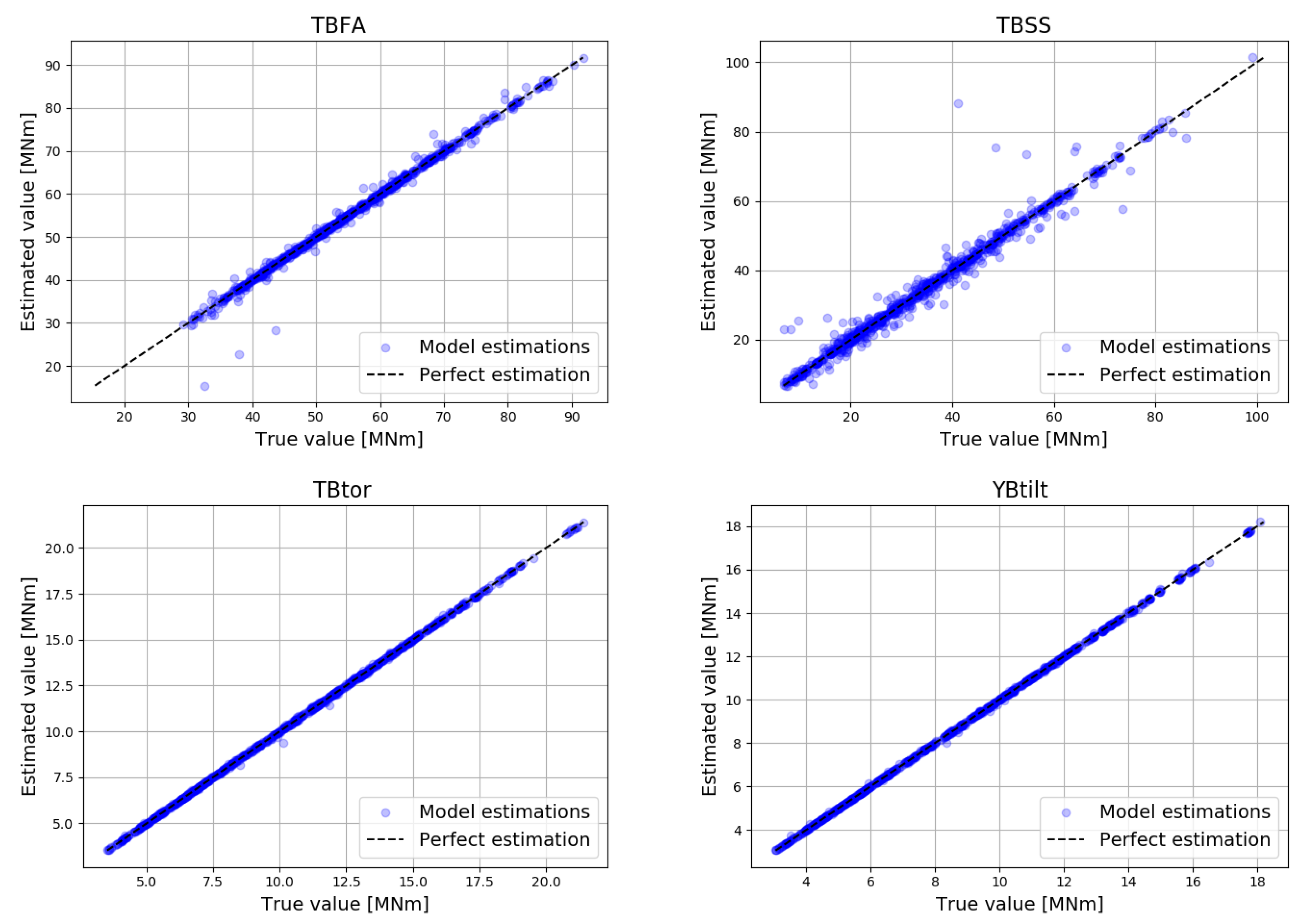
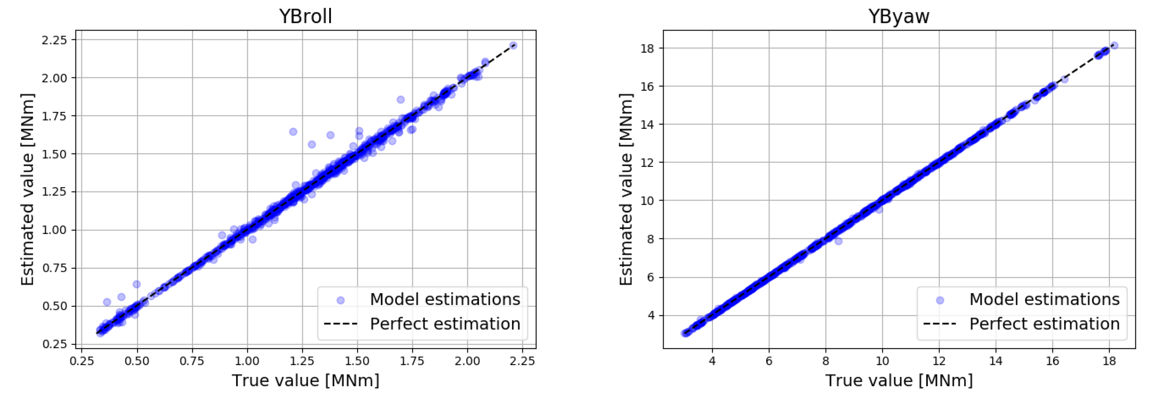
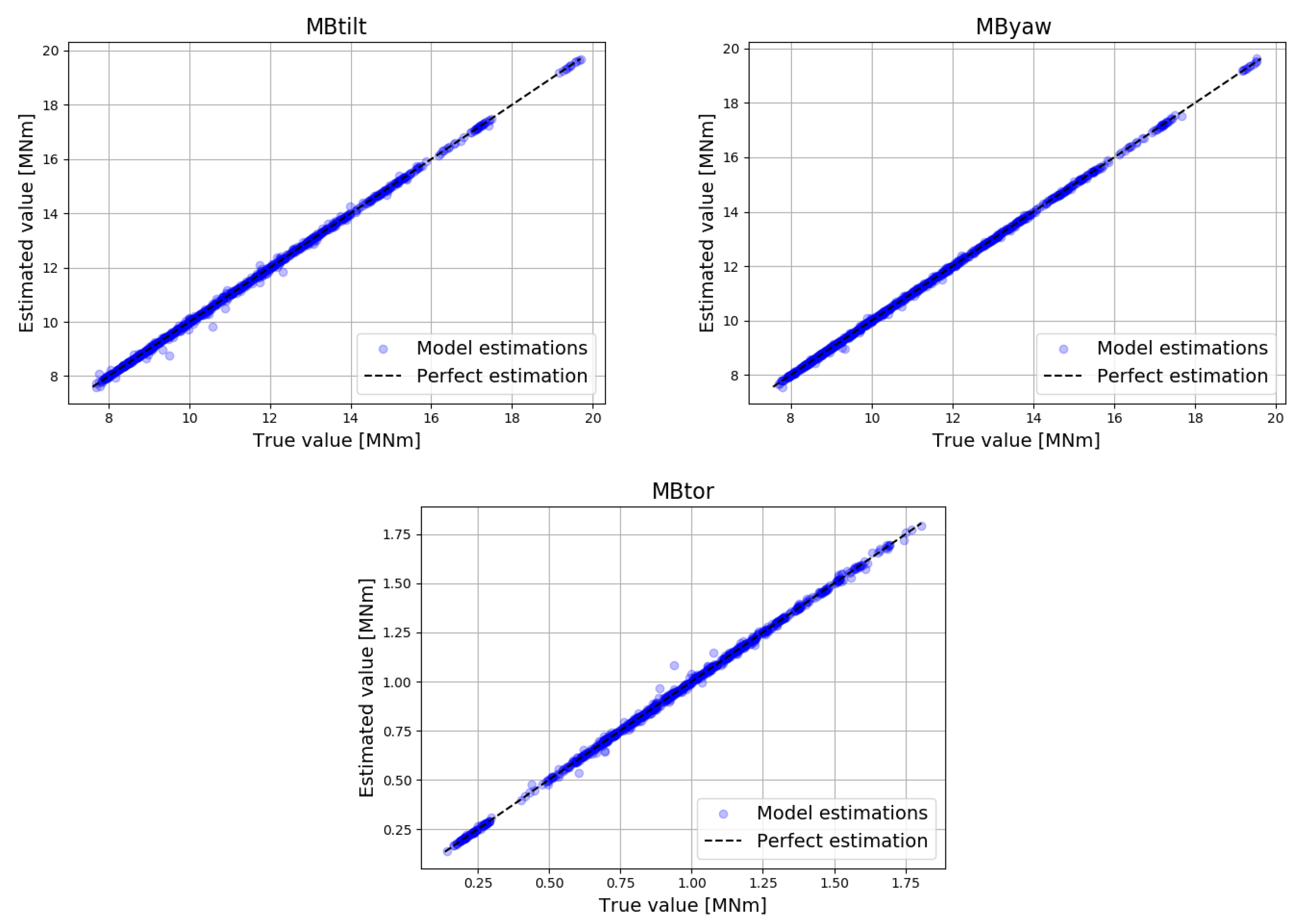
In Linear Regression (LR), for all the prediction variables, the NRMSE are relatively big. This is as expected as the trend of the prediction variables tends to be non-linear. The only prediction variable that has relatively small error is BRedge. This is due to the fact that BRedge of short term DELs has linear trend and it is mainly affected by gravity. In Artificial Neural Network (ANN), the NRMSE for many of the predicted short term DELs of the load channels and electrical power are higher than the Linear Regression model. More specifically, the ANN has better performance than Linear Regression only in the predicted short-term DELs of BRtor, YBroll and MBtor. Artificial Neural Networks is supposed to have the ability to learn and model non-linear and complex relationships. With this in mind, it would be expected that the ANN would have greater performance than Linear Regression. This is not the case because of the small data set (825 samples). To determine if the ANN model over-fits, the relationship between training and test error was observed. Moreover, the ANN model was tested in a holdout data set. These procedures could not give a valid proof that the model over-fits due to the small training and test sample. When the sample for testing is small, there is a possibility that the model behaves well in this specific small test sample but fails to capture the overall performance. As other studies have shown in many scientific fields [29,30], ANN typically have poor performance in complex problems with a limited number of training cases. In this specific case, the ANN has too many parameters to fit properly and therefore Linear Regression is more robust and outperforms ANN [31]. In Gaussian Process Regression (GPR), the NRMSE for most of the predicted variables is significantly lower in comparison to the other two models. More specifically, the NRMSEs for electrical power and BRedge, TBtor, YBtilt, YByaw, MBtilt, MByaw short-term DELs are below 1%, whereas BRflap, BRtor, TBFA and MBtor are below 2%. The outlier is TBSS, which gives a relatively high NRMSE of 8.3%. These results indicate that the Gaussian Process Regression model has high accuracy and can be trusted to predict with this (relative small) input data set, the electrical power and short DEL of a small wind farm. The scatter plots of the estimated variables against the simulated loads and electrical power are shown in Figure 4, Figure 5, Figure 6 and Figure 7. In these scatter plots in many cases, the results show that the GPR method gives a relative good prediction of the target variables.

4.2. Performance Evaluation of Gaussian Process Regression: Full Data Set

As previously discussed, Gaussian Process Regression has high accuracy in the prediction of short DELs and electrical power. However, due to uncertain nature of data, the model may result in better accuracy but fail to realise the data properly and hence performs poorly when the data set is varied. This means that the model is not robust enough and hence its usage is limited. Given these facts, a test was made in order to observe exactly the behaviour of the model for specific features. More specifically, by using all the observations for testing and training the model, at I ref = 0.12 and normal operating upstream wind turbine (set-point of upstream wind turbine = 1), the test error is given in Figure 8 and Figure 9. The test error is defined as follows.
e = | y y ^ | y
where y ^ denotes the estimate of the observation variable y.
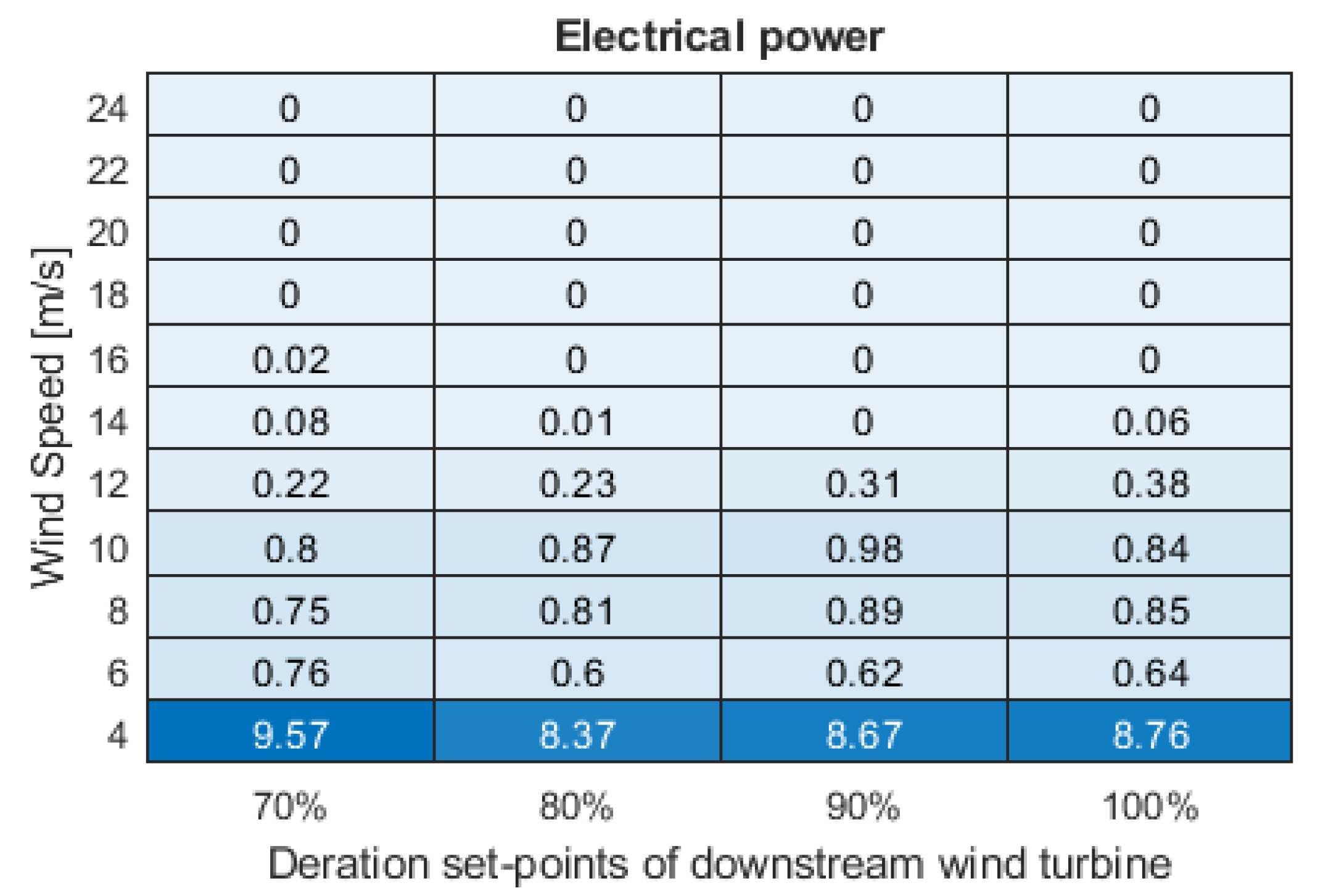
As it is observed, the highest error (12%) that is found in this model is when the prediction variable is TBSS, the wind speed is 10 m/s and the downstream wind turbine is operating at 100%. The test errors of the rest of prediction variables including the electrical power shown in Figure 9 are small. Similar trends have been also found for the other two turbulence intensities of 0.14 and 0.16, while in this paper we only show the results for turbulence intensity of I ref = 0.12 .

4.3. Performance Evaluation of Gaussian Process Regression: Various Size of Input Data Set

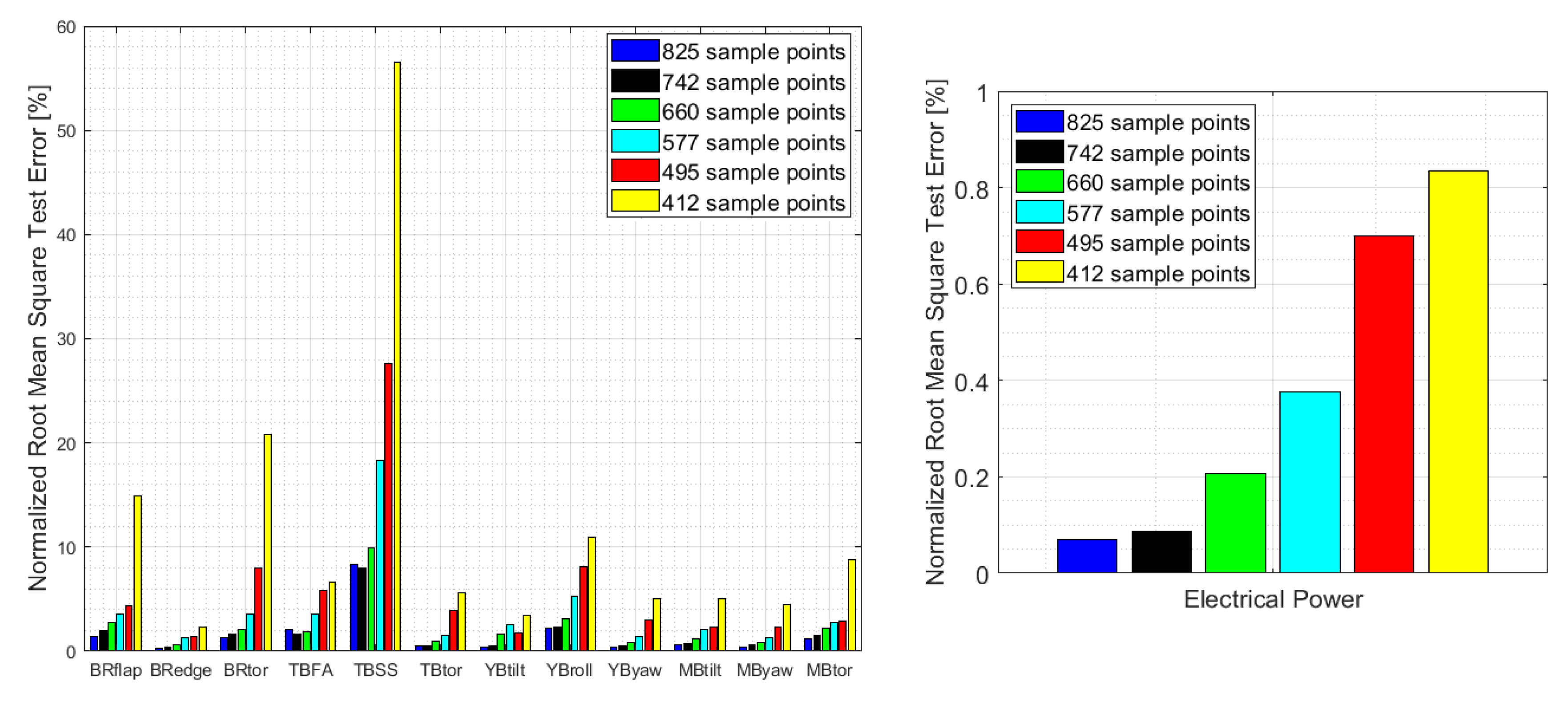
To capture the behaviour and evaluate the performance of the Gaussian Process Regression, the model was trained and tested in smaller input data sets. In Figure 10, the NRMSE for different input sample points can be seen. The training samples were chosen randomly from the full data set of 825 samples. The models were trained with 90%, 80%, 70%, 60% and 50% of 825 samples. Model trained with full size data set is shown as a benchmark.
In Figure 10, the link between the error of the model and size of samples is clearly demonstrated, where the NRMSE is getting higher when the input data set is smaller. The GPR model demonstrated promising results. For example, in the results with 660 sample points, the fatigues for all structural components were with less than 10% of NRMSEs while the power was with 0.2% of NRMSE. Eventually, it is the choice of system designers to determine the number of training samples they use based on the accuracy needed by their applications.

4.4. Performance Evaluation of Gaussian Process Regression: Test Model by Unknown Input Data Set

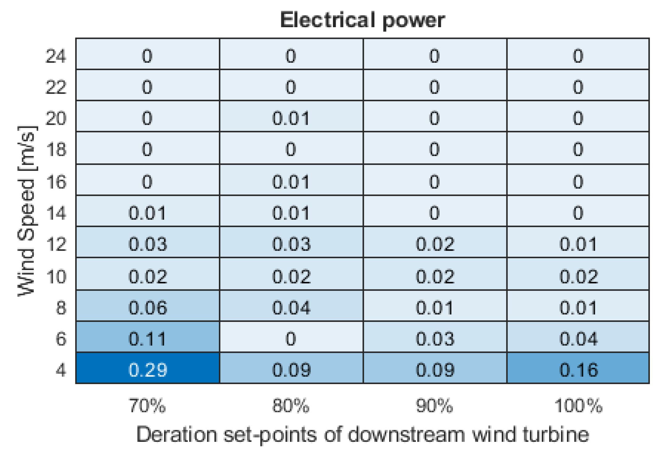
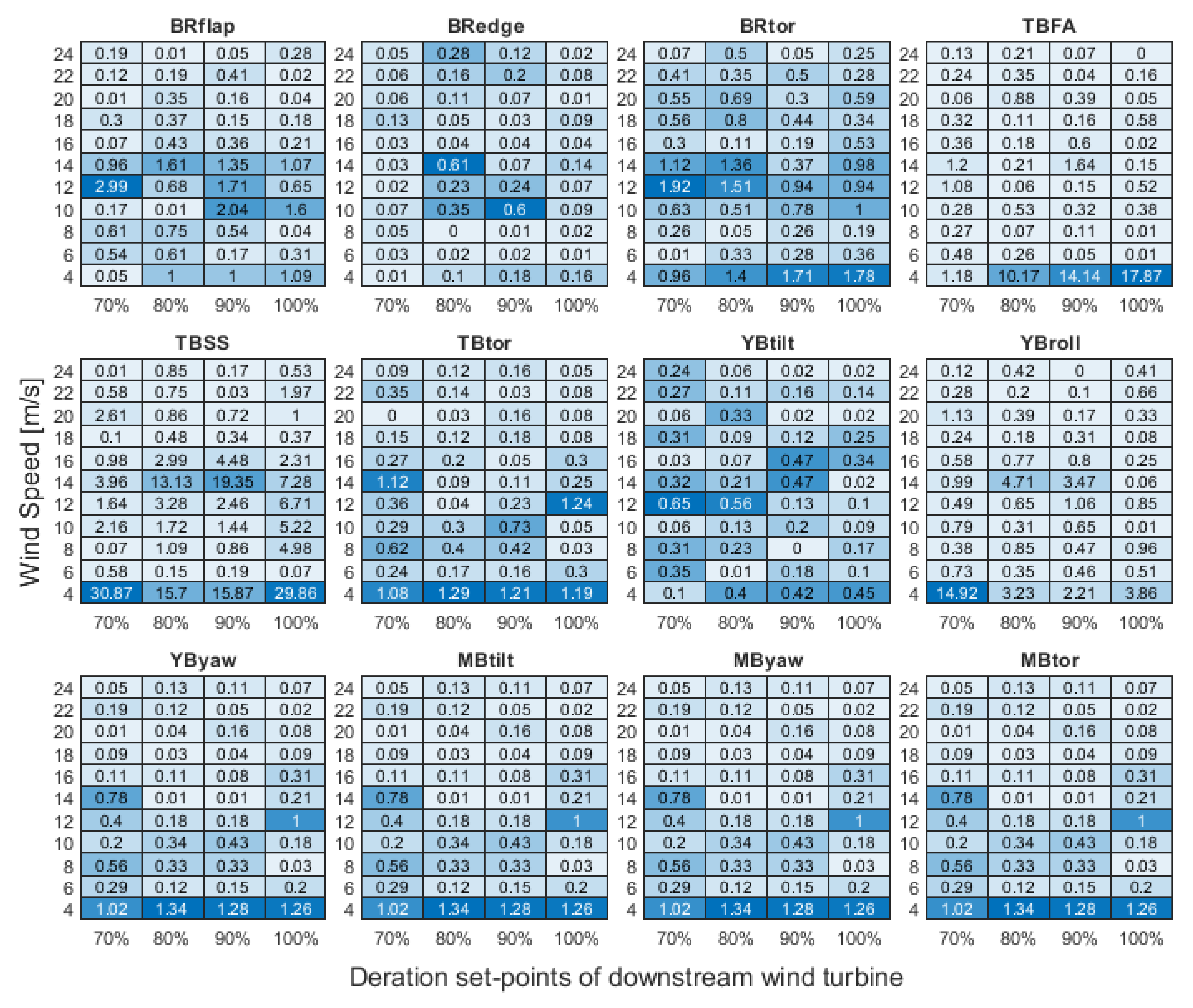
Finally, the last test of the model was made with an unknown input data set. This input data set was not used for training the model but only for testing it. This input data set did not contain features of all the wind speeds (11 different wind speeds) with turbulence intensities (3 different turbulence intensities) I ref = 0.12 , 0.14 , 0.16 and all deration set-points of downstream wind turbine (70%, 80%, 90% and 100%). Correspondingly, the number of samples that were excluded was 11 × 3 × 4 = 132 . As a result, from the initial full data set of 825 samples, the previously mentioned 132 sample points were not included and therefore the input data set consisted of 693 observations. The model was saved and tested in a specific case, where I ref = 0.14 and set-point of upstream wind turbine at 90%. The results are shown in Figure 11 and Figure 12. In this way, this specific case is not included in the training procedure of the model and therefore the test error of this new unknown data can show how robust the model is. In general, the results are promising, where the NRMSEs for loads and electrical power are relatively small. For some channels, for example, power, the highest test error occurs at the lowest wind speeds and especially at 4 m/s. Nonetheless, for wind farm load re-balancing, load surrogate models are typically employed in the above-rated wind conditions.

5. Conclusions

A fast and efficient procedure to construct a surrogate model has been presented for predicting the power and fatigue loads of turbines in a wind farm. The surrogate model was built based on results from a high fidelity aero-elastic simulation including the wake effect. Three regression methods, namely, Linear Regression, Artificial Neural Network and Gaussian Process Regression, have been investigated. Among three regressions, the model trained by Gaussian Process Regression has achieved superior accuracy based on a given small amount of training samples. Furthermore, for GPR, the relationship between accuracy and number of training data samples has been demonstrated. The result revealed that with 660 samples, for a case of two turbines, the GPR is able to provide accurate predictions within 10% errors for all turbine structural loads and 0.2% errors for the power. Future work will look into the possibility to extend the proposed approach by adding more turbines in a wind farm and furthermore, add observation noise so that different sample points are corrupted by different degrees of noise.

Author Contributions

The paper was a collaborative effort among the authors. G.G.: conceptualization, methodology, software, investigation, writing—original draft preparation; W.H.L.: conceptualization, writing—original draft preparation, supervision, project administration; F.M.: conceptualization, data curation, writing—original draft preparation, supervision. All authors have read and agreed to the published version of the manuscript.

Funding

This research was partially funded by the ForskEL Programme under project PowerKey—Enhanced WT control for Optimised WPP Operation (Grant No. 12558).

Conflicts of Interest

The authors declare no conflict of interest.

References

  1. Boersma, S.; Doekemeijer, B.; Gebraad, P.; Fleming, P.; Annoni, J.; Scholbrock, A.; Frederik, J.; van Wingerden, J.W. A tutorial on control-oriented modeling and control of wind farms. In Proceedings of the 2017 American Control Conference (ACC), Seattle, WA, USA, 24–26 May 2017; pp. 1–18. [Google Scholar]
  2. Frederik, J.; Weber, R.; Cacciola, S.; Campagnolo, F.; Croce, A.; Bottasso, C.; van Wingerden, J.W. Periodic dynamic induction control of wind farms: Proving the potential in simulations and wind tunnel experiments. Wind Energy Sci. 2020, 5, 245–257. [Google Scholar] [CrossRef] [Green Version]
  3. Munters, W.; Meyers, J. Towards practical dynamic induction control of wind farms: Analysis of optimally controlled wind-farm boundary layers and sinusoidal induction control of first-row turbines. Wind Energy Sci. 2018, 3, 409–425. [Google Scholar] [CrossRef] [Green Version]
  4. Annoni, J.; Gebraad, P.M.O.; Scholbrock, A.K.; Fleming, P.A.; van Wingerden, J.W. Analysis of axial-induction-based wind plant control using an engineering and a high-order wind plant model. Wind Energy 2016, 19, 1135–1150. [Google Scholar] [CrossRef]
  5. Raach, S.; Schlipf, D.; Cheng, P.W. Lidar-based wake tracking for closed-loop wind farm control. J. Phys. Conf. Ser. 2016, 753, 052009. [Google Scholar] [CrossRef] [Green Version]
  6. Fleming, P.; Annoni, J.; Scholbrock, A.; Quon, E.; Dana, S.; Schreck, S.; Raach, S.; Haizmann, F.; Schlipf, D. Full-Scale Field Test of Wake Steering. J. Phys. Conf. Ser. 2017, 854, 012013. [Google Scholar] [CrossRef]
  7. Soleimanzadeh, M.; Wisniewski, R.; Kanev, S. An optimization framework for load and power distribution in wind farms. J. Wind Eng. Ind. Aerodyn. 2012, 107–108, 256–262. [Google Scholar] [CrossRef] [Green Version]
  8. Zhang, B.; Soltani, M.; Hu, W.; Hou, P.; Chen, Z. A wind farm active power dispatch strategy for fatigue load reduction. In Proceedings of the American Control Conference, Boston, MA, USA, 6–8 July 2016; pp. 5879–5884. [Google Scholar]
  9. Liu, Y.; Wang, Y.; Wang, X.; Zhu, J.; Lio, W.H. Active power dispatch for supporting grid frequency regulation in wind farms considering fatigue load. Energies 2019, 12, 1508. [Google Scholar] [CrossRef] [Green Version]
  10. Mirzaei, M.; Soltani, M.; Poulsen, N.K.; Niemann, H.H. Model based active power control of a wind turbine. In Proceedings of the 2014 American Control Conference, Portland, OR, USA, 4–6 June 2014; pp. 5037–5042. [Google Scholar]
  11. Lio, W.H.; Mirzaei, M.; Larsen, G.C. On wind turbine down-regulation control strategies and rotor speed set-point. J. Phys. Conf. Ser. 2018, 1037, 032040. [Google Scholar] [CrossRef] [Green Version]
  12. Lio, W.H.; Galinos, C.; Urban, A. Analysis and design of gain-scheduling blade-pitch controllers for wind turbine down-regulation. In Proceedings of the 2019 IEEE 15th International Conference on Control and Automation (ICCA ), Edinburgh, UK, 16–19 July 2019. [Google Scholar]
  13. Frandsen, S. Turbulence and Turbulence Generated Fatigue in Wind Turbine Clusters; Technical Report Risø-R-1188; Risø National Laboratory: Roskilde, Denmark, 2007. [Google Scholar]
  14. Keck, R.E.; de Maré, M.; Churchfield, M.J.; Lee, S.; Larsen, G.; Madsen, H.A. Two improvements to the dynamic wake meandering model: Including the effects of atmospheric shear on wake turbulence and incorporating turbulence build-up in a row of wind turbines. Wind Energy 2015, 18, 113–132. [Google Scholar] [CrossRef]
  15. Larsen, G.C.; Madsen, H.A.; Thomsen, K.; Larsen, T.J. Wake meandering: A pragmatic approach. Wind Energy 2008, 11, 377–395. [Google Scholar] [CrossRef]
  16. Larsen, T.J.; Madsen, H.A.; Larsen, G.C.; Hansen, K.S. Validation of the dynamic wake meander model for loads and power production in the Egmond aan Zee wind farm. Wind Energy 2013, 16, 605–624. [Google Scholar] [CrossRef] [Green Version]
  17. Dimitrov, N. Surrogate models for parameterized representation of wake-induced loads in wind farms. Wind Energy 2019, 22, 1371–1389. [Google Scholar] [CrossRef]
  18. Mendez Reyes, H.; Kanev, S.; Doekemeijer, B.; van Wingerden, J.W. Validation of a lookup-table approach to modeling turbine fatigue loads in wind farms under active wake control. Wind Energy Sci. 2019, 4, 549–561. [Google Scholar] [CrossRef] [Green Version]
  19. Galinos, C.; Kazda, J.; Lio, W.H.; Giebel, G. T2FL: An efficient model for wind turbine fatigue damage prediction for the two-turbine case. Energies 2020, 13, 1306. [Google Scholar] [CrossRef] [Green Version]
  20. Bak, C.; Zahle, F.; Bitsche, R.; Yde, A.; Henriksen, L.C.; Natarajan, A.; Hansen, M.H. Description of the DTU 10 MW Reference Wind Turbine; Technical Report-I-0092; DTU Wind Energy: Roskilde, Denmark, 2013. [Google Scholar]
  21. Larsen, T.J.; Hansen, A.M. How 2 HAWC2, the User’s Manual; Technical Report; DTU Wind Energy: Roskilde, Denmark, 2019. [Google Scholar]
  22. Glauert, H. Airplane Propellers. In Aerodynamic Theory; Springer: Berlin/Heidelberg, Germany, 1935; pp. 169–360. [Google Scholar]
  23. Meng, F.; Lio, A.W.H.; Liew, J. The effect of minimum thrust coefficient control strategy on power output and loads of a wind farm. J. Phys. Conf. Ser. 2020, 1452, 012009. [Google Scholar] [CrossRef] [Green Version]
  24. Downing, S.D.; Socie, D.F. Simple rainflow counting algorithms. Int. J. Fatigue 1982, 4, 31–40. [Google Scholar] [CrossRef]
  25. Pedregosa, F.; Varoquaux, G.; Gramfort, A.; Michel, V.; Thirion, B.; Grisel, O.; Blondel, M.; Prettenhofer, P.; Weiss, R.; Dubourg, V.; et al. Scikit-learn: Machine Learning in Python. J. Mach. Learn. Res. 2011, 12, 2825–2830. [Google Scholar]
  26. Paszke, A.; Gross, S.; Massa, F.; Lerer, A.; Bradbury, J.; Chanan, G.; Killeen, T.; Lin, Z.; Gimelshein, N.; Antiga, L.; et al. PyTorch: An Imperative Style, High-Performance Deep Learning Library. In Advances in Neural Information Processing Systems 32; Wallach, H., Larochelle, H., Beygelzimer, A., d’Alché-Buc, F., Fox, E., Garnett, R., Eds.; Curran Associates, Inc.: New York, NY, USA, 2019; pp. 8024–8035. [Google Scholar]
  27. Murphy, K.P. Machine Learning: A Probabilistic Perspective; MIT Press: Cambridge, MA, USA, 2013. [Google Scholar]
  28. Rasmussen, C.; Williams, C. Gaussian Processes for Machine Learning; MIT Press: Cambridge, MA, USA, 2006. [Google Scholar]
  29. Keshari, R.; Ghosh, S.; Chhabra, S.; Vatsa, M.; Singh, R. Unravelling Small Sample Size Problems in the Deep Learning World. In Proceedings of the 2020 IEEE Sixth International Conference on Multimedia Big Data (BigMM), New Delhi, India, 24–26 September 2020; IEEE Computer Society: Los Alamitos, CA, USA, 2020; pp. 134–143. [Google Scholar]
  30. Bataineh, M.; Marler, T. Neural network for regression problems with reduced training sets. Neural Netw. 2017, 95, 1–9. [Google Scholar] [CrossRef]
  31. Van der Ploeg, T.; Austin, P.; Steyerberg, E. Modern modelling techniques are data hungry: A simulation study for predicting dichotomous endpoints. BMC Med. Res. Methodol. 2014, 14, 137. [Google Scholar] [CrossRef] [PubMed] [Green Version]
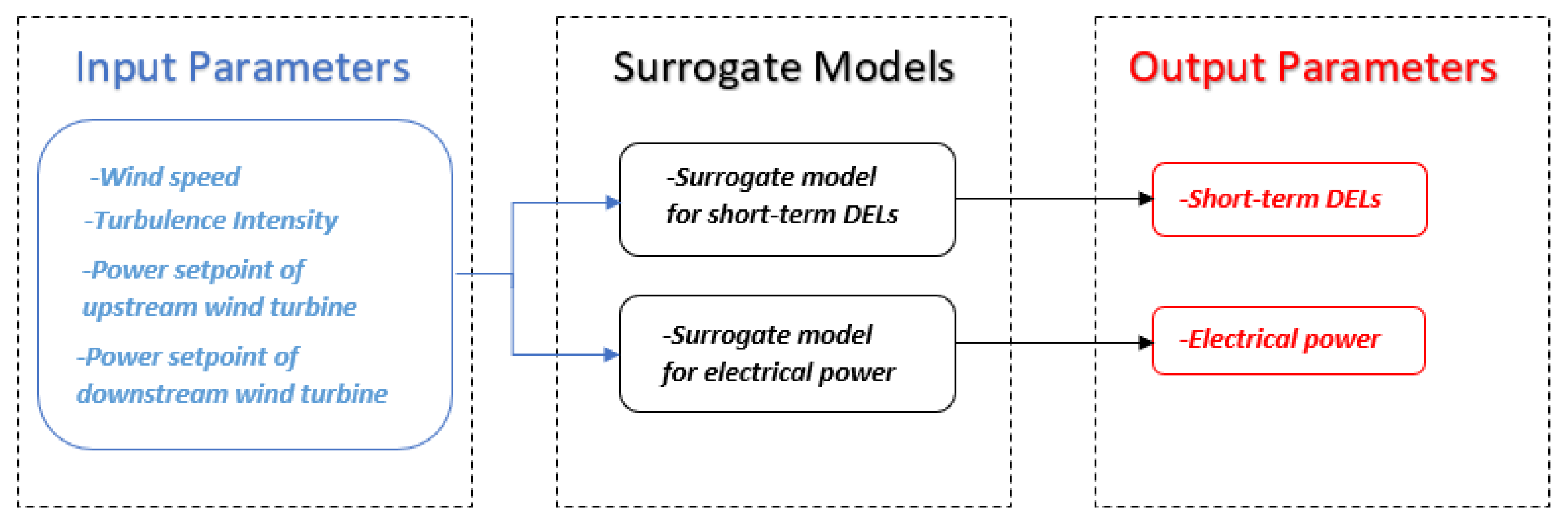
Figure 1. General schematic diagram of surrogate models.
Energies 13 06360 g001
Figure 2. Artificial Neural Network schematic diagram with four inputs, ten hidden units and one output.
Energies 13 06360 g002
Figure 3. Normalised root mean squared error (NRMSE) for all predicted variables for Linear Regression (LR), Artificial Neural Network (ANN) and Gaussian Process Regression (GPR).
Energies 13 06360 g003
Figure 4. Electrical power, BRflap, BRedge and BRtor estimated and observed values for GPR method.
Energies 13 06360 g004
Figure 5. TBFA, TBSS, TBtor and YBtilt estimated and observed values for GPR method.
Energies 13 06360 g005
Figure 6. YBroll and YByaw estimated and observed values for GPR method.
Energies 13 06360 g006
Figure 7. MBtilt, MByaw and MBtor estimated and observed values for GPR method.
Energies 13 06360 g007
Figure 8. Test error of GPR for all DELs of different deration set-points of downstream wind turbine (x-axis) at I ref = 0.12 with normal operating upstream wind turbine. The model was trained and tested by all input data set.
Energies 13 06360 g008
Figure 9. Test error of GPR electrical power of different deration set-points of downstream wind turbines (x-axis) at I ref = 0.12 with normal operating upstream wind turbine. The model was trained and tested by all input data set.
Energies 13 06360 g009
Figure 10. NRMSE of GPR for all DELs (left) and electrical power (right) for different sample points.
Energies 13 06360 g010
Figure 11. Test error of GPR for all DELs of different deration set-points of downstream wind turbines at I ref = 0.14 with operating upstream wind turbine at 90%. The model was trained and tested in an input data set that does not contain input data of I ref = 0.12 , 0.14 , 0.16 and downstream wind turbines at 70%, 80%, 90% and 100%.
Energies 13 06360 g011
Figure 12. Test error of GPR for electrical power of different deration set-points of downstream wind turbines at I ref = 0.14 with operating upstream wind turbine at 90%. The model was trained and tested in an input data set that does not contain input data of I ref = 0.12 , 0.14 , 0.16 and downstream wind turbines at 70%, 80%, 90% and 100%.
Energies 13 06360 g012
Table 1. Input variables for surrogate models.
ParametersValuesNumber of Samples
Wind Speed U ¯ [m/s]4, 6, 8, 10, 12, 14, 16, 18, 20, 22, 2411
Turbulence intensity reference I ref [-]0.12, 0.14, 0.16×3
Upstream down-regulation level δ d , up [-]0.00, 0.60, 0.70, 0.80, 0.90, 1.00 × ( 5 + 5 × 4 )
Downstream down-regulation level δ d , down [-]0.70, 0.80, 0.90, 1.00
Total number of samples825
Publisher’s Note: MDPI stays neutral with regard to jurisdictional claims in published maps and institutional affiliations.