Emergy Based Decoupling Analysis of Ecosystem Services on Urbanization: A Case of Shanghai, China

Abstract

In order to respond to rapid urbanization, understanding the relationships between urbanization and ecosystem services (ESs) is of practical importance to move toward sustainable urban development. In this study, an emergy-GIS based method is proposed to evaluate ESs. Spatiotemporal emergy values of water retention (WR), air purification (AP), carbon sequestration (CS), soil conservation (SC), and biodiversity conservation (BC) were quantified and relationships among these ESs were analyzed by taking China’s largest city, Shanghai, as a case. The decoupling analysis was conducted to study the relationship between urbanization and ESs. Results show that the total value of regulating ESs had declined by 8.24% from 2005 to 2010. Chongming had the largest value of ESs, followed by Pudong. There is a synergetic relationship among AP, CS, and SC, while a tradeoff appears between WR and other services. Irregular “U” shape relationships between the decrease of ESs and urbanization indicators were observed. Results from decoupling analysis show that ESs experienced weak decoupling from urbanization in most districts. Finally, policy implications were raised based on the study results.

1. Introduction

The world is experiencing unprecedented urban growth. According to a report from the United Nations [1], over 4 billion population lived in cities in 2015, accounting for 54% of the world’s total population. Furthermore, it is projected that six out of 10 people will live in cities by 2030. The urbanization rate has risen more sharply in developing countries [2]. In China, accompanying with rapid economic growth since the reform and opening policies enacted in 1978, the urbanization rate increased from 17.92% in 1978 to 58.52% in 2017, while the urban area had a significant increase from 9775 km² in 1985 to 56,225 km² in 2017 [3,4]. As the engine of economic growth, spurring domestic demand and catalyzing regional development [5], China’s urbanization is expected to reach 80% in 2050 [6]. Although rapid urbanization boosted China’s economic development, the huge increase in population density (36% of the nation’s land hosts 96% of the total population, especially in Eastern China [5]) and the tremendous change of land use (built-up area increased from 13,148 km² in 1990 to 40,058 km² in 2010 [7]) has considerable impacts on ecosystems. The benefits people obtained from ecosystems, termed as ecosystem services (ESs), are essential for human survival [8]. In 1997, two seminal publications boosted the studies on ES [9,10]. In 2005, the Millennium Ecosystem Assessment (MA) further contributed to the great progress in this field. More recently, the increasing political interest in ES promoted national ES assessments worldwide, including the UK National Ecosystem Assessment (NEA), China’s first national ecosystem assessment (2000–2010) [11], and Russia’s National Ecosystem Assessment [12], etc., Urban ESs are the services directly produced by ecological structures within urban areas or peri-urban regions [13]. In order to address the challenges brought by rapid urbanization, it is critical to prepare more appropriate urban policies so that cities can become more inclusive, safe, resilient, and sustainable. This requires a holistic understanding of the relationship between urbanization and ESs so that the major challenges can be identified. It is also consistent with the sustainable development goal (SDG) 11 since 102 SDG targets are identified in relationship with urban ecosystems [14]. In 2012, the Chinese government adopted ecological civilization as the national development strategy, aiming to correct the GDP-based policy and guide economic and social development toward sustainable development, and strengthen ecosystem protection and governance. In particular, president Xi has decided to further pursue ecological civilization [15].

Academically, many studies have been conducted in this field. For example, Wan et al. [16] developed an urbanization indicator system and evaluated the urbanization process and the related ESs. They found that an irregular inverse “U” relationship exists between urbanization and ESs in Huaibei, a mineral resource-based city in Anhui province. Su et al. [17] studied the response of ES changes to urbanization from 1994 to 2006 in Shanghai by using a geographically weighted regression (GWR) and proxy-based approach and identified significant spatial autocorrelation for the patterns of ESV changes. Zhou et al. [18] analyzed the relationship between urbanization and ESs in the Jing-jin-ji (JJJ) urban agglomeration and found that increases in waterways, forests and orchards greatly offset the decrease of ESs caused by urban sprawl. Wang et al. [19] studied the relationship between ES and urbanization in the Beijing-Tianjin-Hebei (BTH) urban mega-region by employing a curve estimation method, in which urbanization is indicated by GDP density, population density, and the developed land proportion. Their results show that ESs and urbanization levels both increased. Lyu et al. [20] found that urbanization results in increased crop production, carbon storage, nutrient retention, and sand fixation in rural areas, but leads to decreased crop production, carbon storage, nutrient retention, and habitat quality in developing urban areas. Li et al. [21] demonstrated that urbanization in Nanjing has a spatially heterogeneous impact on ESs. Zhang et al. [22] adopted the bivariate Moran’s I method to study the spatial correlations between ESs and urbanization in Wuhan, Their results show that there are negative spatial correlation between ESs and urbanization. Tian et al. [23] identified thresholds of ES response to the urbanization of the peri-urban area in Beijing by using a piecewise linear regression method. By adopting the Residential Environment Assessment Tool to value ecosystem services, Radford and James [24] found that the major ecosystem services exist at lower values within urban areas in the Greater Manchester region. Song and Deng [25] found a 34.66% ecosystem service value loss from 1988 to 2008 due to the conversion from cultivated land to urban areas in the North China Plain. Delphin et al. [26] established urbanization scenarios in two disparate watersheds in Florida and found that the value of carbon storage and timber volume both decreased while the value of water yield increased. Sirakaya et al. [27] found that biodiversity restorations play a key role to provide ecosystem services in an urbanized world. Ferreira et al. [28] employed the benefit transfer method to quantify ecosystem service value and found that loss of arboreal vegetation caused by urbanization was the key factor of the ecosystem service value decline in the eco-tone area of Paraiba. Eigenbrod et al. [29] modeled the urban land-use change in Britain and predicted the related ecosystem services in 2031, in which their results demonstrated the significant losses of carbon sequestration and agricultural production under the urban sprawl growth scenario.

These studies demonstrate that the relationships between ESs and urbanization differ significantly due to the different urbanization modes and ESs quantification methods. In general, ESs assessment is the prerequisite for accurate analysis. There are two main approaches to assess ESs. The first is based on monetary valuations such as market price and willingness to pay, which captures the values of ESs anthropocentrically. Globally, Costanza et al. [9] estimated that the economic value of 17 global ecosystem services was US$ 16–54 trillion per year in 1995 $US. Later in 2014, they updated the economic value of global ecosystem services for the year 2011 to be $125 trillion/yr [30]. However, such an economic approach is too narrow to capture the holistic picture of ESs [31]. The second is based on biophysical accounting (non-monetary). Many studies adopted the Integrated Valuation of Ecosystem Services and Tradeoffs models (InVEST) model to evaluate the biophysical values of ESs [11,32,33,34,35], while others employed the ecological modeling methods such as ecological footprint [36] and emergy accounting (EMA) [37,38]. Emergy is defined as “the available energy of one kind of previously used up directly and indirectly to make a service or product” [39]. Focusing on the role of the environment in support of human-dominated processes, EMA based studies quantify the natural ecosystem’s contribution to produce ESs and identify the quality differences of different resource flows. In this regard, Pulselli et al. [40] analyzed the relationship between ESs and emergy flows and found that nature is more efficacious in producing ecosystem services than economic systems in producing GDP. Coscieme et al. [41] demonstrated that renewable emergy and ESs are strongly correlated within the national territory. Grönlund et al. [42] proposed two methods based on EMA to assess ESs, i.e., the natural driving forces and ecosystem function. Besides, EMA has been adopted to analyze ESs for various ecosystems, such as Maryland forests [43,44], subtropical forests and plantations restoration [45], Jing-Jin-Ji forest ecosystem [46], Erhai Lake [47], aquatic ecosystem [48] and mining systems [49]. Within urban systems, EMA has been integrated with GIS to study the spatiotemporal dynamics of land use, natural resources and ESs, including Campania Region [50], Abruzzo Region [51], the greater Taipei area [52], and Chongming Island [22].

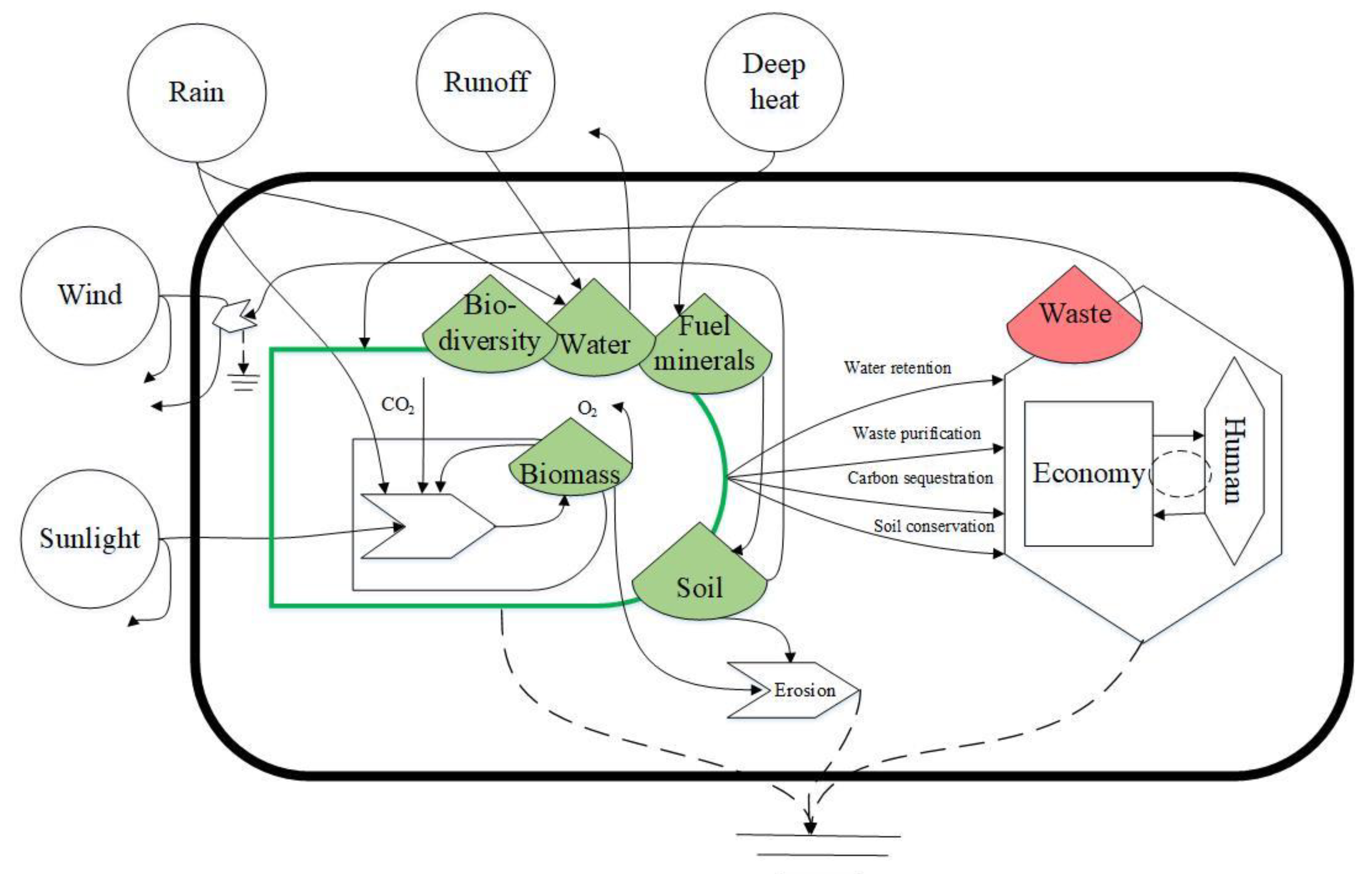
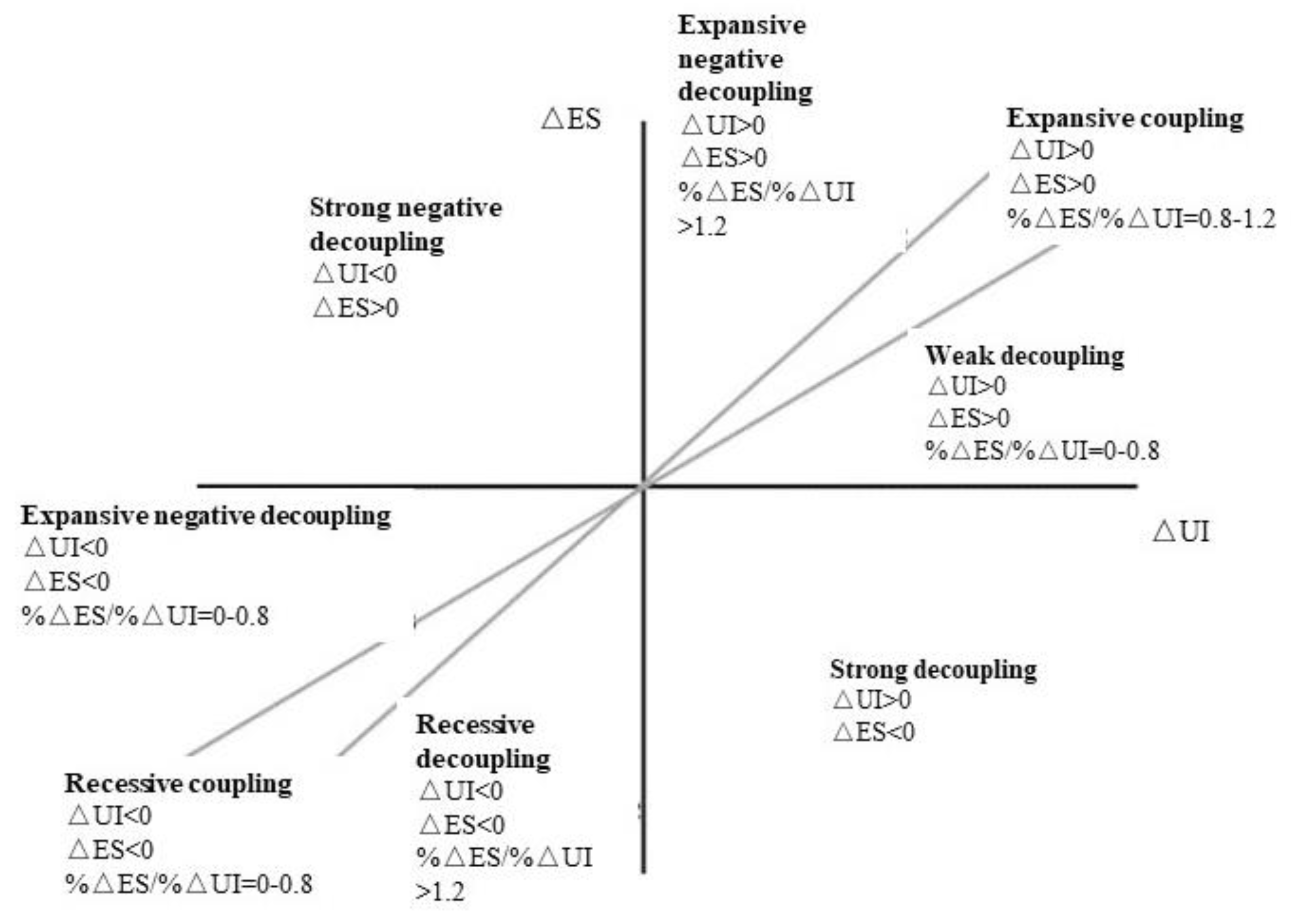
These previous studies illustrate that the EMA method is a supply-side ESs evaluation method, which highlights the donor-side value of ESs and complements traditional economic assessment. However, few EMA based studies have been carried out to study the relationships between urbanization and ESs. To fill such a research gap, this study proposes an ESs accounting framework based on EMA and GIS. Decoupling analysis, introduced by OECD [53] and later improved by Tapio [54], was combined with a curve estimation method to characterize the relationships since the results are more applicable to communicate [55,56,57,58]. As one of the most urbanized cities in China and the world, Shanghai is taken as a case study city. Specifically, this study aims to answer the following questions:

• What are the spatiotemporal dynamic changes of emergy values of ESs in Shanghai?
• What are the relationships among different ESs during the process of urbanization?
• What is the relationship between urbanization and ESs in Shanghai?

The paper is organized as follows. After this introduction section, Section 2 presents the city of Shanghai, related data sources, and research methods. Section 3 presents the research results and research limitations. Finally, Section 4 draws research conclusions and raises policy implications.

2. Methods and Data

2.1. Case Study City and Data Sources

Shanghai city is located in the easternmost region of the Yangtze River Delta. It is one of the most advanced and urbanized cities in China and the world. Figure 1 shows the location of Shanghai in China and its administrative districts. Shanghai occupies an area of 6340.5 km² with a total population of 24.15 million in 2018. Its main geomorphic types include the western lacustrine plain, the eastern coastal plain, the central Huangpu River plain, and the estuarine delta [59,60]. Driven by rapid economic growth, Shanghai has experienced robust urbanization accompanied by various environmental challenges (

Table 1. Urbanization indicators of Shanghai between 2005 and 2010 [62].

Years	Registered Population (Million)	Migrant Population (Million)	GDP (100 Million Yuan)	Primary Industry (100 Million Yuan)	Secondary Industry (100 Million Yuan)	Tertiary Industry (100 Million Yuan)	Buildup Land (m2)
2005	13.60	4.38	9154.18	80.34	4452.92	4620.92	1.65 × 109
2010	14.04	8.97	17,165.98	114.15	7218.32	9833.51	2.01 × 109

). The Shanghai municipal government is ambitious to protect its local ecosystem. In February 2017, the Shanghai municipal government announced it will designate more than 40% of its land area as natural areas without any further development [32]. In November 2017, the State Council approved the Shanghai Master Plan for the period of 2017–2035, in which the forest coverage rate will increase from 15% in 2015 to 23% in 2035 and the per capita green space will increase from 7.6 m^2. in 2015 to 13 m² in 2035. This ambitious goal demonstrates that Shanghai aims to move toward sustainable development.

2.2. Data Sources

Given the interdisciplinary nature of this study, the required data should come from various sources, including governmental documents, statistical yearbooks, and research papers. Such data can be categorized into biophysical and socioeconomic types. The land cover data at a spatial resolution of 30 m × 30 m were provided by the Data Center for Resources and Environmental Sciences at the Chinese Academy of Sciences (http://www.resdc.cn). Precipitation data, the net primary productivity (NPP), sunshine duration, and wind speed data, both at 1 km × 1 km spatial resolution, were supplied by the National Earth System Science Data Sharing Infrastructure of China (http://www.geodata.cn). Evapotranspiration data at a spatial resolution of 1 km × 1 km from MOD16A3 were supplied by NASA-USGA (http://files.ntsg.umt.edu/data/NTSG_Products/MOD16/). Social and economic data, including spatial distribution of population and GDP, both at 1 km × 1 km spatial resolution, were obtained from the Data Center for Resources and Environmental Sciences, Chinese Academy of Sciences (http://www.resdc.cn). Runoff coefficients and species density (indigenous to China and endangered) were obtained from Ouyang et al. [11]. Data on ecosystem capacity to purify pollutants were from Wang et al. [19], Liu and Yang [63], and Zhang et al. [64]. Data of biomass in ecosystems were from Bai et al. [32]. Data related to soil conservation, including rainfall erosivity factors, soil erodibility factors, topographic factors, and cover-management factors, were from Teng [65]. The period of 2005–2010 was chosen as the study period due to data availability.

2.3. Emergy-GIS Based Evaluation on ESs

Emergy measures the contributions from both nature and humans to production based upon the environmental work required to support a system’s dynamics [66]. By focusing on nature’s investment, the complete role of the natural system as a source, sink, and regulator can be identified when conducting emergy analysis [67]. Unit Emergy Values (UEVs), which is the equivalent solar emergy (sej) input to generate a unit of output, convert all flows and stocks into emergy so that the distinctions between qualities of resources can be enabled. The total annual emergy input to the biosphere is defined as a geobiosphere emergy baseline (GEB). The updated 12.00 × 10²⁴ sej/yr value was adopted as the GEB for this study [66]. Integrating the GIS tool into emergy analysis can uncover the spatiotemporal dynamic changes of ESs. When adopting an emergy-GIS-based method to account for ESs, the following procedures should be taken.

2.3.1. Identification of the Study Boundaries and Related ESs Provided by Local Ecosystems

Since the purpose of this study is to evaluate urban ESs and analyze the relationship between urbanization and ESs, the boundary of this study is set as the administrative region of Shanghai city. The landscape was classified into 6 categories, including forest land, grassland, crop land, water area, buildup land, and unused land. Bai et al. [32] identified (1) water retention; (2) water purification; (3) carbon sequestration; (4) soil conservation, and; (5) biodiversity conservation as the priority ESs in Shanghai. Beyond these ESs, this study also takes air purification into consideration due to the severe ambient air pollution in Shanghai [68]. The related ESs provided by local ecosystems are referred to in

Table 2. Land types and considered ecosystem services (ESs) in this study.

Ecosystem Services	Forest	Cropland	Grassland	Water	Buildup Land	Unused Land
1.  Water conservation	1	1	1	1	1	1
2.  Air, water and soil purification	1	1	1	1
3.  Carbon sequestration	1	1	1
4.  Soil conservation	1	1	1		1	1
5.  Biodiversity conservation	1	1	1	1	1	1

Note: The “1” in the table means ESs considered produced by different land-use types.

.

2.3.2. An Emergy-GIS-Based Framework to Evaluate Ecosystem Services

An emergy flow diagram can reflect various flows and stocks of the studied system. Figure 2 shows the emergy flow diagram of Shanghai urban ESs. The renewable inputs, the role of the ecosystem and the urban system, and the main ecological processes among them are illustrated. After drawing this emergy flow diagram, the emergy based equations are raised to quantify ESs into emergy by considering the related ecological processes. The related UEVs and their sources in this study refer to

Table A5. UEVs used in this study based on 12.0 × 10²⁴ sej/yr emergy baseline.

Items	UEVs	Reference
1.  Solar radiation	1 sej/J	By definition
2.  Geothermal heat	4.90 × 103 sej/J	[66]
3.  Tidal energy	3.09 × 104 sej/J	[66]
4.  Wind, kinetic energy	7.90 × 102 sej/J	[66]
5.  Rain, chemical potential	7.01 × 103 sej/J	[66]
6.  Runoff, geopotential energy	1.28 × 104 sej/J	[66]
7.  Runoff, chemical potential	2.13 × 104 sej/J	[66]
8.  Wave energy	4.20 × 103 sej/J	[66]
9.  Soil	1.42 × 1010 sej/kg	[31]
10.  Fresh water	1.00 × 108 sej/kg	[31]
11.  Biomass (2005)	7.27 × 108 sej/kg	This study
12.  Biomass (2010)	7.57 × 108 sej/kg	This study

(Appendix A). Finally, the spatial emergy values of ESs are assigned and mapped by using GIS.

(1)

Water retention

Water retention refers to the ecosystem’s ability to intercept or store water resources from natural precipitation [32]. It is crucial to keep an adequate freshwater supply in Shanghai so that local citizens can benefit. The equation proposed by Jia et al. [69] is adopted to account emergy of water retention service, as shown in Equation (1):

$$E_{wr} = \left(P-ET\right)\times A\times UE{V}_{water}$$

(1)

$E_{wr}$ is the emergy of water retention, P is natural precipitation, ET is local evapotranspiration, A is the area of the ecosystem as defined by land cover, UEV_water is the UEV value of water.

(2)

Air, water, and soil purification

Due to the purification ability of the local ecosystem, the adverse impacts of emissions on the environment and public health can be reduced. In this study, we adopt the accounting framework proposed by Yang et al. [46] to quantify these services. The reduced impacts (air, water, and soil purification services provided by urban ecosystems) are quantified by integrating Disability Adjusted Life Years (DALYs) and Potentially Disappeared Fraction (PDF) into emergy [46,70,71]. DALYs can be considered as a measurement of the gap between current health status and an ideal health situation where the entire population lives to an advanced age, free of disease and disability [72]. Potentially Disappeared Fraction (PDF) measures emissions’ impacts on ecosystem quality which can be considered as the fraction of species with a high probability of no occurrence in a region due to unfavorable conditions [46,73]. The following equations quantify emissions’ impacts into emergy.

$$E_{mHH} = {{\displaystyle \sum }}^{ }{M}_i\times DAL{Y}_i\times {\tau }_H$$

(2)

$$E_{mEQ}={{\displaystyle \sum }}^{ }{M}_i\times PD{F}_i\times E_{Bio}={{\displaystyle \sum }}^{ }{M}_i\times PD{F}_i\times MAX\left(R_i\right)$$

(3)

Max(R_i) = Max (Sum (sunlight, deep heat, tidal energy), wind energy, wave energy, rain (chemical potential energy), runoff (geopotential and chemical potential energy))

(4)

$$E_{mE}=E_{mHH}+E_{mEQ}$$

(5)

where E_mHH is the emergy required to reduce harmful effects on public health (sej); M_i is the capacity of local ecosystem to purify the i-th pollutant (kg/yr),

Table A1. The capacities of ecosystems to purify pollutants.

Land Types	SO2 (kg/hm2)	PM10 (kg/hm2)	PM2.5(kg/hm2)	NOx	Fluoride	Mcu	Mmn	Mzn	Mpb
Forest land	97.73	10.67	2.65	6.80	8.99	-	-	-	-
Grassland	79.7097	1.7994	-	-	-	27.7	1823.1	94.4	46.6
Crop land	45.00	1.0999	-	33.25	0.48	-	-	-	-

(See Appendix A) lists the detailed values of M_i; DALY_i is the disability-adjusted life year of one individual caused by i-th air pollutant (cap yr/kg); ${\tau }_H$ is the per capita used emergy (sej/cap). ${\tau }_H$ in Shanghai equals to 2.30 × 10¹⁶ sej/capital and 2.37 × 10¹⁶ sej/capital in 2005 and 2010, respectively (recalculated from [60]). $E_{mEQ}$ is the emergy required to reduce emissions’ impact on ecosystem quality (sej). PDF_i indicates the potential fraction of species affected by the i-th emission (PDF × ha × yr × kg⁻¹),

Table A2. Pollutants considered and the related impacts.

Items	Damage Category to Human Health	DALYs/kg of Emission	Damage to Ecosystem	PDF m2 yr
SO2	Respiratory effects	5.46 × 10−5	Acidification and eutrophication	1.04
PM2.5	Respiratory effects	7.00 × 10−4	-	-
PM10	Respiratory effects	3.75 × 10−4	-	-
NOx	Respiratory effects	8.87 × 10−5	Acidification and eutrophication	5.71
Fluoride	Climate change	7.48 × 10−4	-	-
Cu	-	-	Ecotoxic substances	10.81
Mn	-	-	-	-
Zn	-	-	Ecotoxic substances	22.66
Pb	-	-	Ecotoxic substances	0.09

(Appendix A) lists the detailed values of DALY and PDF. E_Bio is the emergy of stored biological resource per unit area [49], which equals to $MAX\left(R_i\right)$ [46]. $E_{mE}$ is the sum of $E_{mHH}$ and $E_{mEQ}$, which denotes the total emergy required to reduce all the emissions’ impacts.

According to the State Forestry Administration of the People’s Republic of China [74], water pollutant absorbed by local ecosystems can be calculated as follows:

$$M_w=Q_i\times \left(c_{input,i}-c_{output,i}\right)$$

(6)

where M_W is the i-th pollutant absorbed by water area (kg/yr); $Q_i$ is emission amount of pollutant i (kg/yr); $c_{input,i}$ is the concentration of pollutant i in water inlet (%) and $c_{output,i}$ is the concentration of pollutant i in the water outlet (%). This study ignores water pollutant purification services since the data related to water pollutant concentrations, including DALYs and PDF parameters, are lacking. Additionally, water quality monitoring is beyond the scope of this study.

(3)

Carbon sequestration

In order to respond to global climate change, it is of great importance to increase the carbon sink. Especially, Shanghai is considered as the most vulnerable Chinese city facing climate change due to its low-lying character [32]. The following equations can account for carbon sequestration of ecosystems into emergy [46].

$$E_{mCS}={{\displaystyle \sum }}^{ }0.5\times \frac{B_i}{T}\times A_i\times UE{V}_{bio}$$

(7)

$$UE{V}_{bio}=\frac{E_{mNPP}/S}{NPP}$$

(8)

$$E_{mNPP}=MAX\left(R_i\right)= \mathrm{Max} (\mathrm{Sum} (\mathrm{sunlight}, \mathrm{deep} \mathrm{heat}, \mathrm{tidal} \mathrm{energy}), \mathrm{wind} \mathrm{energy}, \mathrm{wave} \mathrm{energy}, \mathrm{rain} (\mathrm{chemical} \mathrm{potential} \mathrm{energy}), \mathrm{runoff} (\mathrm{geopotential} \mathrm{and} \mathrm{chemical} \mathrm{potential} \mathrm{energy}\left)\right)$$

(9)

where $E_{mCS}$ is the emergy of carbon sequestration, B_i is the amount of biomass in ecosystem classified by landscape i, T is the turnover time of biomass (one year estimated from Odum [39]), A_i is the area of the related ecosystem of land use type i, S is the area of the studied city. The amount of carbon sequestration is estimated as half of the biomass, and UEV_Bio is the unit emergy value of biomass [46].

(4)

Soil conservation

Soil erosion is a national dilemma in China. In particular, the Yangtze River Basin suffers the most [32]. Located in the Yangtze River Delta, Shanghai is also suffering from soil erosion. In this study, we assess the soil conservation service based on the Revised Universal Soil Loss Equation (RUSLE) [75], shown in Equations (10) and (11).

$$SC=R\times K\times LS\times \left(1-C\times P\right)$$

(10)

$$E_{SC}=SC\times UE{V}_{soil}$$

(11)

where SC is the soil retention capacity (t ha⁻¹ a⁻¹), R represents the rainfall erosivity factor (MJ mm ha⁻¹ h⁻¹ a⁻¹), K is the soil erodibility factor (t ha h ha⁻¹ MJ⁻¹ mm⁻¹), LS is the slope-length and steepness factor, C is the cover-management factor, and P is the conservation practices factor.

Table A4. The parameters related to soil conservation in Shanghai.

	Forest Land	Grassland	Crop Land	Buildup Land	Water Area	Unused Land
C	0.11	0.5	0.21	0.27	-	0.77
LS	0.1	0.1	0.1	0.1	-	0.1
P	1	1	0.01	1	-	1
R(MJ mm ha−1 h−1 yr−1	4594.66	4594.66	4594.66	4594.66	-	4594.66
K(t ha h ha−1 MJ−1 mm−1)	0.038	0.038	0.038	0.038	-	0.038

(See Appendix A) lists the values of these parameters. UEV_soil is the UEV of soil.

(5)

Biodiversity conservation

Maintaining biodiversity is crucial for the sustainable productivity of land due to its core role to provide ecosystem functions and services [76,77]. Equation (12) can account for the emergy required by biodiversity conservation [46].

$$E_{bc}=N_1\times S\times \left(GEB\times T\right)/N_0$$

(12)

where E_bc represents the emergy required by biodiversity conservation (sej); N₁ is the species density in the study area (No./ha); S is the area of the study system (ha); GEB is the geobiosphere emergy baseline (GEB) (sej/yr); T is the average turnover time of species (yr) (3 million years); N₀ is the number of global species (8.7 million species [78]). Only the value of 2010 is considered in this study due to the lack of data for other years.

2.4. Trade-Off and Synergy among ESs

Studying the relationship among multiple ESs is of particular importance to identify win-win outcomes for ESs management [79]. Two interaction relationships of ESs have been identified, i.e., trade-off and synergy. Trade-off indicates that the provision of one ES is reduced as a result of another increased ES, while synergy reflects that multiple ESs are enhanced simultaneously [80]. This study quantifies the different values of ESs between 2005 and 2010 to investigate the relationships, i.e., ${\mathrm{ES}}_{\mathrm{i}, 2010}-{\mathrm{ES}}_{\mathrm{i}, 2005}$. Grid-scaled ESs data are extracted to conduct this calculation. Scatter diagrams are employed to demonstrate the relationships between two ESs. A point that appeared in the first or third quadrant indicates that the ESs are increased or decreased simultaneously, which can be classified as synergy. While a point that appears in the second or fourth quadrant, means that one ES is reduced as a result of another increased ES, which can be classified as trade-offs.

2.5. Relationship between Urbanization Indicators and ESs

Previous studies consider the total GDP of one city as the main indicator to reflect its urbanization level [16,18,21,81]. In this study, the GDP value of the manufacturing industry was adopted due to its great impact on regulating ESs. Other indicators, including population and the built-up land area, are also considered as key factors indicating urbanization. Since various relationships may exist between urbanization indicators and the total ESs, such as linear, logarithm, exponential, power law, and polynomial, the curve estimation method is adopted to determine the relationship [16,19]. We acknowledge that the regression analysis does not establish the causal relationship, but may uncover the dissimilarity or similarity relationship between the variables [43]. Thus, the Tapio decoupling method is employed to study the relationships between urbanization and ESs since it is more applicable to communicate [54]. The traditional Tapio decoupling theory focuses on the undesired output, such as CO₂ and pollutants, while the ES is considered as the desired output in this study. Therefore, the decrease in ESs is adopted. Following Tapio [54], the urbanization elasticity of ESs can be calculated by using Equation (13). The district-level data were extracted to conduct this analysis.

$$\mathrm{Urbanization} \mathrm{elasticity} \mathrm{of} \mathrm{ESs} = \frac{\%△TE{S}_{ }}{\%△UI}$$

(13)

where ΔTES is the decreased value of the total ES during the study period;$△UI$ refers to the changed value of corresponding urbanization indicators, i.e., population, the built-up land, and the GDP of manufacturing industry during the study period. Finally, the degrees of coupling and decoupling of ES influenced by urbanization can be identified according to Figure 3.

3. Results

3.1. Dynamic Changes and Spatial Pattern of Land Use and ESs

Table 3. Land-use change in Shanghai from 2005 to 2010 (m²).

Land Use Types	Area in 2005	Area in 2010	Change Rate (%)
Forest land	1.12 × 108	1.17 × 108	4.31%
Grassland	9.74 × 106	9.74 × 106	0.00%
Crop land	4.19 × 109	3.76 × 109	−10.26%
Buildup Land	1.65 × 109	2.01 × 109	21.72%
Water area	1.95 × 108	1.95 × 108	0.00%
Unused land	1.85 × 108	2.53 × 108	36.88%

shows the changes in land use and land cover (LULC) in Shanghai. During the study period, crop land accounted for the largest proportion, followed by built-up land and water area. During the study period, the area of crop land had decreased by 10.26% from 4.19 × 10⁹ m² in 2005 to 3.76 × 10⁹ m² in 2010, while the area of unused land and built-up land had increased by 36.88% and 21.72%, respectively. Forest land increased by 4.31% from 1.12 × 10⁸ m² in 2005 to 1.17 × 10⁸ m² in 2010. This indicates that the large increases in unused land and built-up land are mainly at the cost of decreased crop land. Figure 4 shows the LULC at the district level, and Figure 5 illustrates the contributions from main districts to land-use changes. For all districts, both built-up land and unused land increased or remained unchanged. Pudong had the most significant change in land use, which contributed 116.68% of total forest land increase, 33.12% of total crop land decrease, 29.95% of total buildup land increase, and 43.04% of the total unused land increase.

Jiading had the second-largest decrease in crop land and increase in built-up land, accounting for 16.24% of total crop land decrease and 18.66% of total built-up land increase, respectively. The largest decrease in forest land occurred in Minhang, which contributed 8.63% of the total forest land decrease. Finally, the maximum water area reduction occurred in Qingpu.

Spatial distributions and changes of the considered ESs are shown in Figure 6, Figure 7, Figure 8, Figure 9 and Figure 10. Spatial values of ESs at the district level were illustrated in Figure 11. For AP, Chongming had the largest contribution, accounting for 21.70% and 23.74% of the total AP in 2005 and 2010, respectively, followed by Pudong and Fengxian. Regarding CS, Chongming had also the largest contribution, accounting for 21.14% and 21.74% of the total in 2005 and 2010, respectively, followed by Pudong and Fengxian. Pudong contributed 19.16% and 18.67% to the total SC in 2005 and 2010, respectively, followed by Chongming and Fengxian. In 2010, Chongming had the highest emergy value of biodiversity, with a figure of 3.14 × 10³⁰ sej, followed by Pudong and Jinshan. When considering the total regulating ESs as a whole, Chongming had the highest value of ESs, with figures of 7.03 × 10¹⁹ sej in 2005 and 6.87 × 10¹⁹ sej in 2010, followed by Pudong (6.67 × 10¹⁹ sej in 2005 and 5.86 × 10¹⁹ sej in 2010), Fengxian (4.21 × 10¹⁹ sej in 2005 and 3.99 × 10¹⁹ sej in 2010), Jinshan (3.62 × 10¹⁹ sej in 2005 and 3.51 × 10¹⁹ sej in 2010), Qingpu (3.46 × 10¹⁹ sej in 2005 and 3.21 × 10¹⁹ in 2010), and Songjiang (3.24 × 10¹⁹ sej in 2005 and 2.95 × 10¹⁹ sej in 2010). Total ESs in all the districts had decreased or remained unchanged. For instance, total ESs in Minhang, Jiading, Baoshan and Pudong had decreased by 18.17%, 16.78%, 14.74% and 12.26% during 2005–2010, respectively. Finally, Pudong contributed 35.31%, 28.78%, and 19.54% of the total-decrease of SC, AP, and WR, respectively. Jiading had the largest contribution to CS decrease, followed by Minhang.

Figure 12 shows the changing trend of different compositions of the total ES, while Figure 13 shows the contributions from different land types. In 2005, SC, CS, AP, and WR contributed 39.34%, 2.33%, 58.36%, and 0.00% to the total ES, respectively. In 2010, SC, CS, AP, and WR contributed 41.71%, 2.56%, 55.76%, 0.00% to the total ES, respectively. AP contributed the most to the total ES, followed by SC and CS, both in 2005 and 2010. The value of the total ES decreased by 8.24% from 3.45 × 10²⁰ sej in 2005 to 3.16 × 10²⁰ sej in 2010. AP decreased by 12.34% from 2.01 × 10²⁰ sej in 2005 to 1.76 × 10²⁰ sej in 2010. SC decreased by 2.74% from 1.36 × 10²⁰ sej in 2005 to 1.32 × 10²⁰ sej in 2010. CS increased by 0.63% from 8.04 × 10¹⁸ sej in 2005 to 8.09 × 10¹⁸ sej in 2010. Finally, WR increased by 10.07% from −1.59 × 10¹⁵ sej in 2005 to −1.43 × 10¹⁵ sej in 2010. Obviously, AP had the largest decrease during the study period. From a land-use point of view, ES from the crop land system contributed the most to the total ES (85.91% in 2005 and 82.24% in 2010), followed by the built-up land (8.68% in 2005 and 11.51% in 2010), and the forest land (4.09% in 2005 and 4.74% in 2010). AP is mainly contributed by the crop land (94.49% in 2005 and 93.60% in 2010), followed by forest land (3.85% in 2005 and 4.61% in 2010). SC is mainly contributed by crop land (75.24% in 2005 and 69.24% in 2010), followed by the builtup land (22.06% in 2005 and 27.61% in 2010). CS is mainly contributed by forest land (48.65% in 2005 and 52.43% in 2010) and crop land (51.14% in 2005 and 47.36% in 2010). Finally, WR is mainly contributed by the water area (46.94% in 2005 and 58.65% in 2010) and the crop land (43.09% in 2005 and 30.31% in 2010). However, the area of crop land had the largest decrease during the study period and there will be a 36.84% decrease in crop land from 2015 to 2035 according to Shanghai Master Plan 2017–2035. Therefore, to compensate for the loss of ESs caused by the decrease of crop land is of great importance.

3.2. ESs Trade-Offs and Synergy

Figure 14 shows the relationships between various ESs. The most points in Figure 14A–C appear in the down-left quadrant, indicating the synergy between these ESs. Figure 14D–F demonstrated the trade-off relationships between WR and other ESs. Correlations among different ESs at the grid level are listed in

Table 4. Pearson correlation coefficient of the regulation of ecosystem services.

	WR	SC	CS	AP
WR	1
SC	−0.105	1
CS	0.065	0.688	1
AP	−0.123	0.975	0.696	1

. The results show that SC and AP had the most correlated relationship, followed by SC and CS. The correlation relationships between WR and others were weak, while negative correlation relationships between WR and AP, WR and SC were observed. Besides, the biodiversity conservation and the total ES were largely correlated in 2010 (Pearson correlation coefficient = 0.979). This result is not surprising since biodiversity plays a core role in producing ESs [32].

3.3. The Impacts of Urbanization on ESs

The spatial changes in grid-scaled GDP and population from 2005 to 2010 are shown in Figure 15.

Table 5. District-level urbanization indicators in Shanghai.

Districts	GDP of Secondary Industry in 2005 (1 × 108 Yuan)	GDP of Secondary Industry in 2010 (1 × 108 Yuan)	Population in 2005 (1 × 104)	Population in 2010 (1 × 104)	Built-up Land in 2005 (1 × 104 m2)	Built-up Land in 2010 (1 × 104 m2)
Chongming	132.66	422.31	65.68	70.34	646	1628
Baoshan	2406.44	2992.43	130.54	190.56	4793	7248
Jiading	1341.72	3465.94	94.28	147.2	3980	7073
Pudong	4673.14	9422.72	367.76	504.73	10,430	18,270
Yangpu	549.76	1046.49	120.32	131.3	4155	4730
Zhabei	223.74	506.76	75.81	83.04	2570	2797
Hongkou	204.31	408.52	78.26	85.23	2874	3192
Putuo	308.08	542.48	110.6	128.88	4262	5146
Qingpu	742.84	1387.87	73.75	108.19	1411	4169
Minhang	1682.98	3779.57	170.76	243.12	6390	12,221
Changning	164.73	286.44	67.18	69.06	2900	3419
Jingan	72.56	84.21	25.65	24.67	1491	1593
Xuhui	787.96	1062.73	98.59	108.52	4187	6332
Songjiang	2060.16	4380.91	88.58	158.34	6318	8109
Fengxian	549.16	1409.92	73.44	108.41	1359	1866
Jinshan	839.07	1542.38	59.21	73.25	1438	2526
Huangpu	336.68	414.2	78.01	67.84	3111	3270

lists the values of urbanization indicators in 2005 and 2010 at the district level. Relationships between the total ES and the urbanization indicators at the district level were explored by using the curve estimations (Figure 16).

The results from the curve estimations show that the increase of urbanization indicators and the decrease of ESs can be characterized by a cubic polynomial, and the irregular “U” shape relationship between the decrease of ESs and the increase of urbanization indicators are observed. In the beginning, with the increase of built-up land and GDP of the manufacturing industry, the decrease of ESs experienced an upward trend. The turning point is observed when the increase in built-up land and GDP of the manufacturing industry reach 2.00 × 10³ and 1.50 × 10³, respectively. The decrease of ESs remains steady before the increase in the built-up land and GDP of the manufacturing industry reach 5.00 × 10³ and 3.00 × 10³. After these points, the decrease of ESs experienced a rapid upward trend. Finally, an overt linear relationship between the decrease of ESs and the increase of population appears.

Figure 17 shows the values of urbanization elasticity of ESs from decoupling analysis at the district level. All elasticity values except the population elasticity in Changning range from 0 to 0.8, indicating the weak decoupling of ESs decrease from urbanization. The value of population elasticity in Changning equals 1.1201, which reflects the expansive coupling of ESs decrease from population growth. Jingan district shows a strong negative decoupling of ESs decrease from population growth, mainly because the population in Jingan declined. According to the decoupling theory, when the two parameters are larger than 0, a larger value of elasticity indicates decreased ESs, reflecting the higher pressure of urbanization on the ecosystem. Besides, when the elasticity value is close to 0.8, it indicates the potential trend toward expansive coupling. Putuo had the largest value of the buildup land elasticity of ESs, with a figure of 0.4454. Banshan had the largest value of GDP elasticity of ESs, with a figure of 0.6052. Changning had the largest value of population elasticity of ESs, indicating the potential expansive coupling trends of ESs decreasing from these urbanization indicators. Finally, the values of urbanization elasticity of ESs in Yangpu, Zhabei, Hongkou, Jingan, Xuhui, and Huangpu are equal to 0, which is mainly because the values of ESs in these districts remain unchanged during the study period.

3.4. Research Limitations and Future Prospective

Due to a lack of sufficient data, this study did not quantify all the ESs, but only those core ESs identified by previous studies. Beyond the considered ESs, the worldwide significant overuses of ESs, such as phosphorus and nutrient cycles, should be also considered in future studies. In addition, this study only quantified the biodiversity conservation for the year 2010, leading to a lack of a dynamic picture of biodiversity conservation. The year 2010 was chosen as the last year of this study because social and economic data (including spatial distributions of GDP and population) are not available for more recent years. Finally, although we proposed this framework to evaluate water pollutant purification services, such a value was not quantified due to the lack of basic data. Further studies can complement these issues when the relevant data are available.

There are several research directions for future studies. Firstly, the impacts of urbanization on ESs demanded by the socioeconomic system and the driving factors can be further studied so that more appropriate recommendations can be raised. Additionally, Shanghai is the most advanced city in China and may have pressure on the broader ecosystem beyond its administrative boundaries, indicating that the teleconnection effect should be taken into consideration in a future study. Finally, it is crucial to further investigate the relationships among fundamental supporting ESs, intermediate ESs, final ESs, and ecosystem structure and functions so that a more complete picture of the ESs process can be uncovered.

4. Conclusions

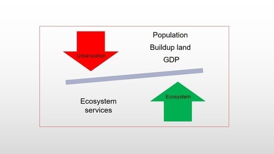
China’s rapid urbanization and economic growth have led to the great change of ecosystem functions. Understanding the relationship between urbanization and ecosystem services is of critical importance to achieving China’s ecological civilization targets and the UN’s SDGs. Under such a circumstance, this study proposes an emergy-GIS-based framework to evaluate the ESs with consideration of the contribution of Shanghai, one of the most economically advanced and populous cities in China and the world. Then, the tradeoffs among different kinds of ESs and the relationships between urbanization indicators and ESs were explored. Finally, a decoupling analysis was conducted to identify the decoupling state of ESs from urbanization.

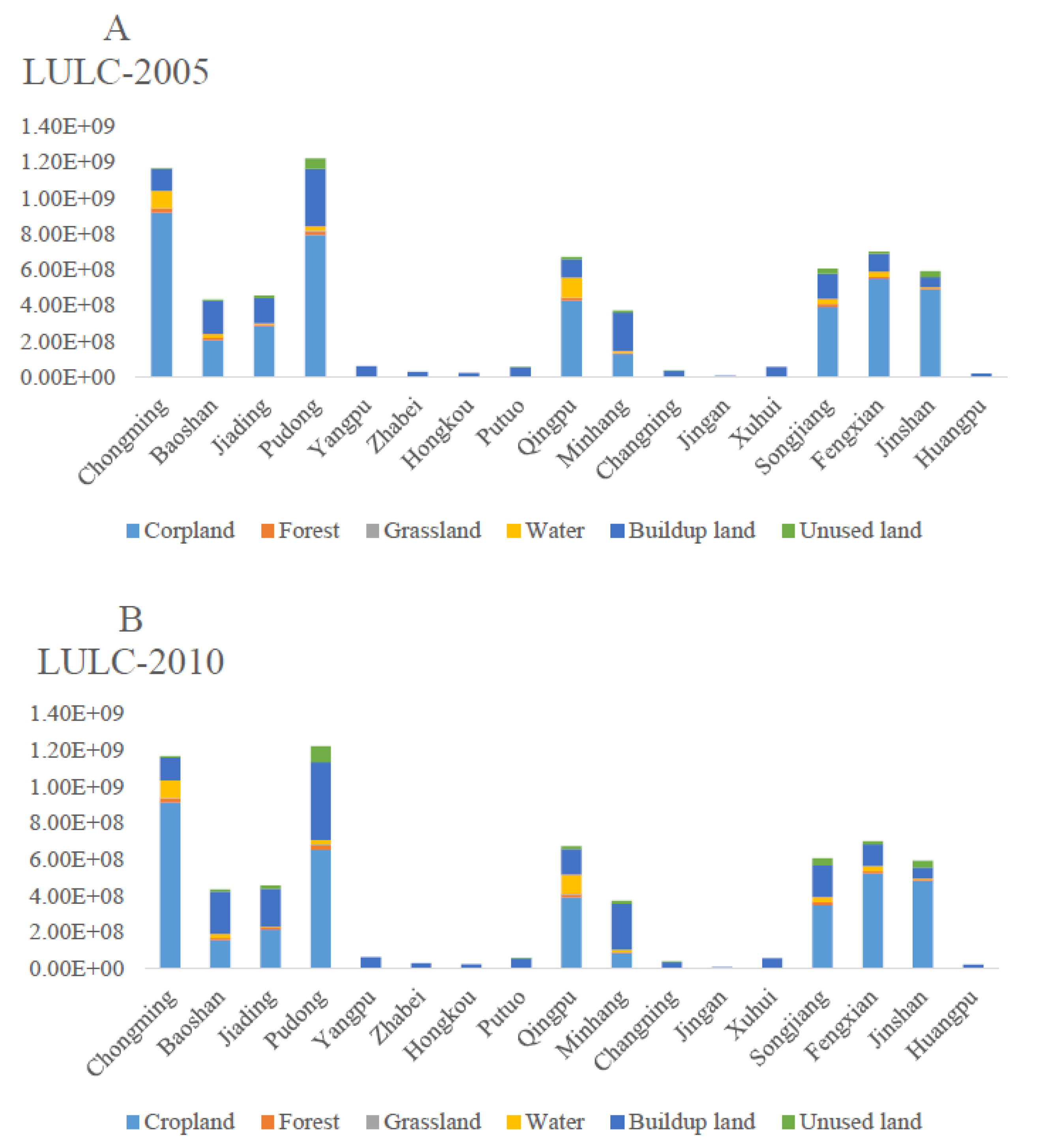
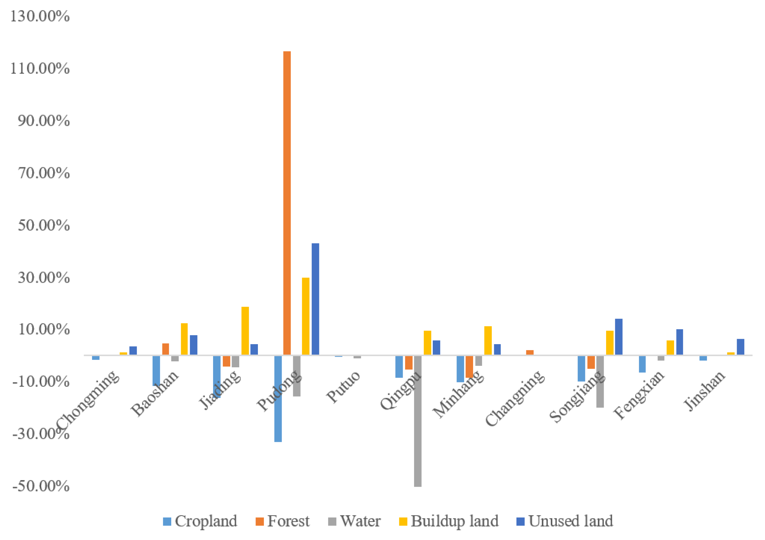
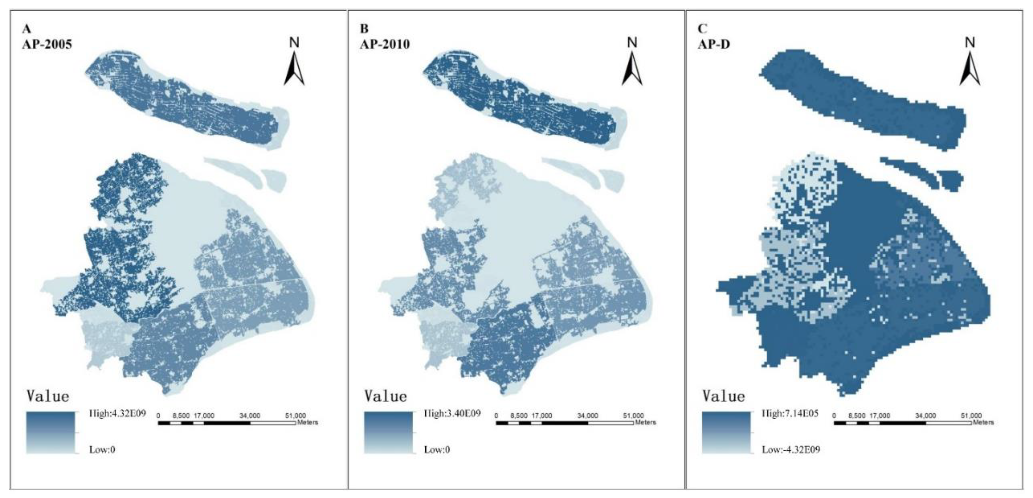
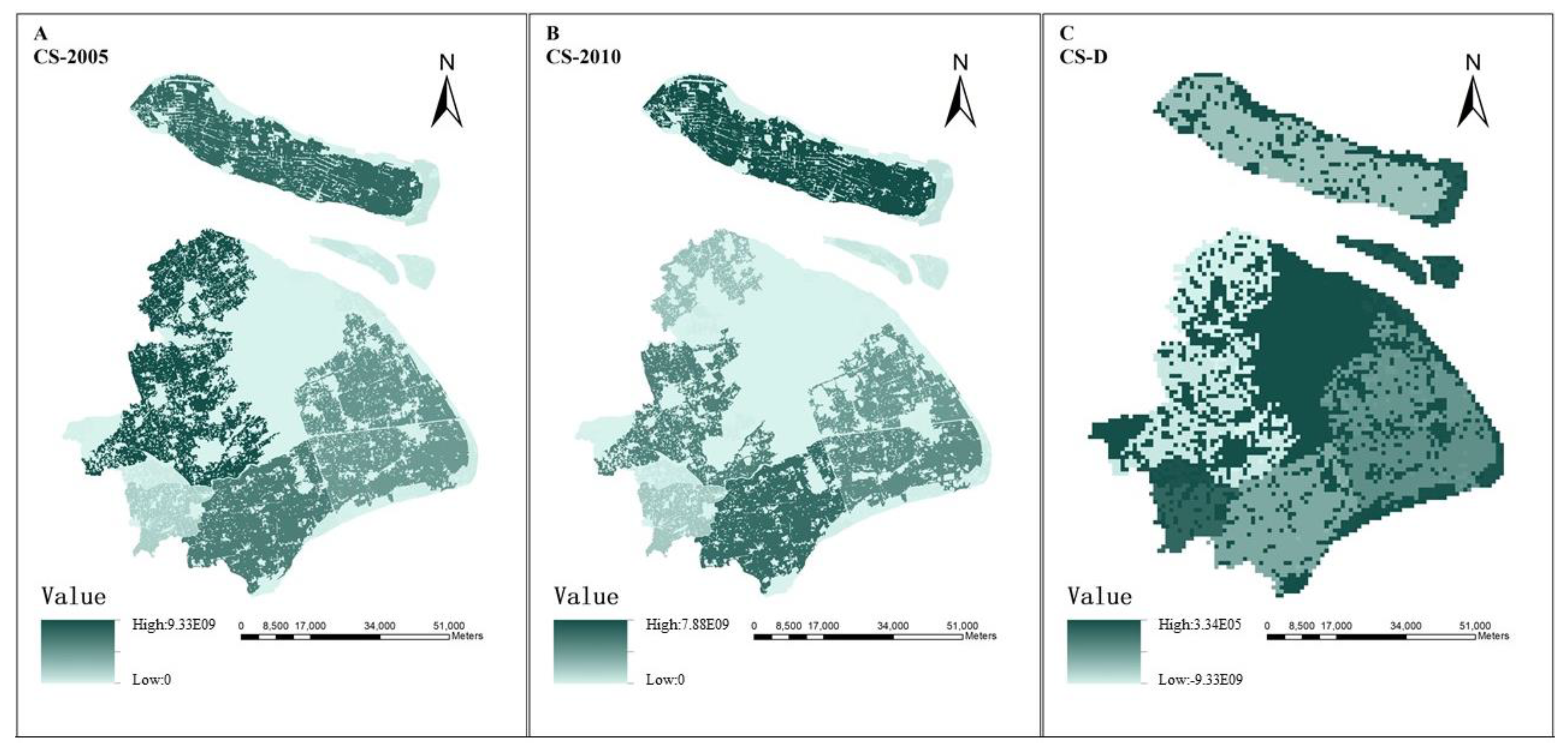
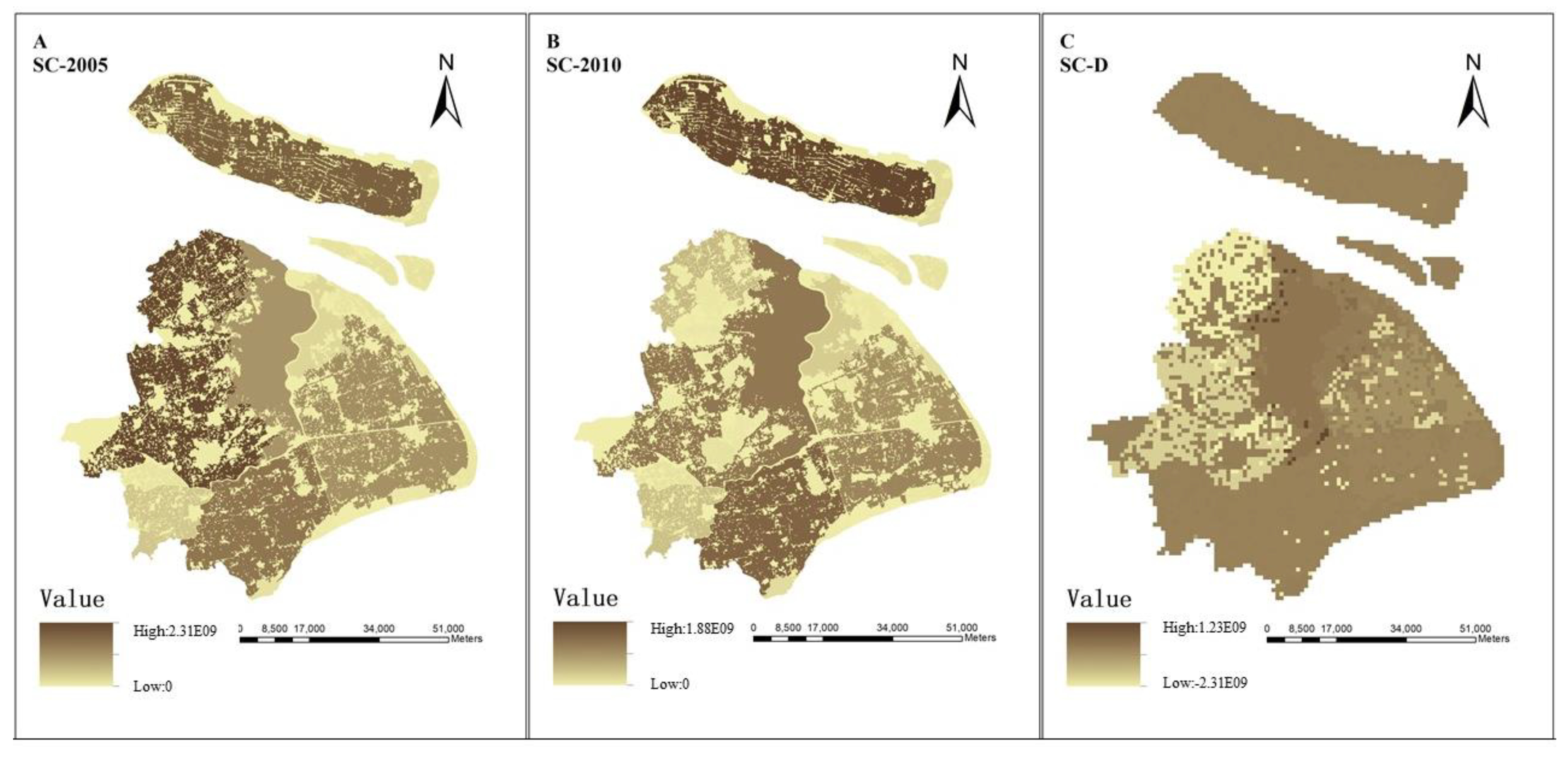
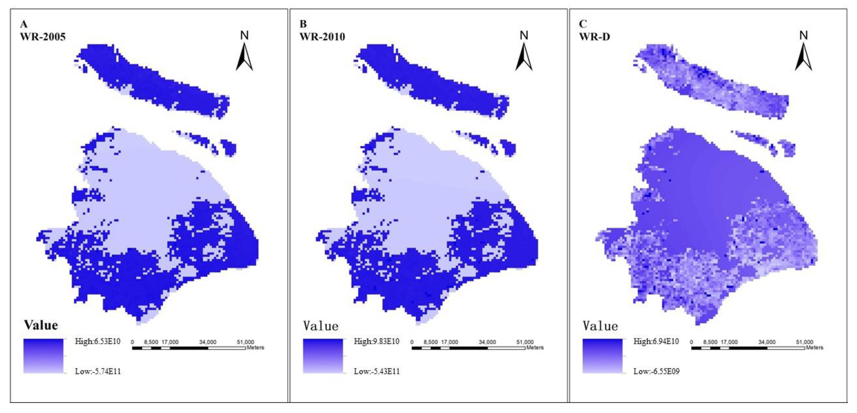
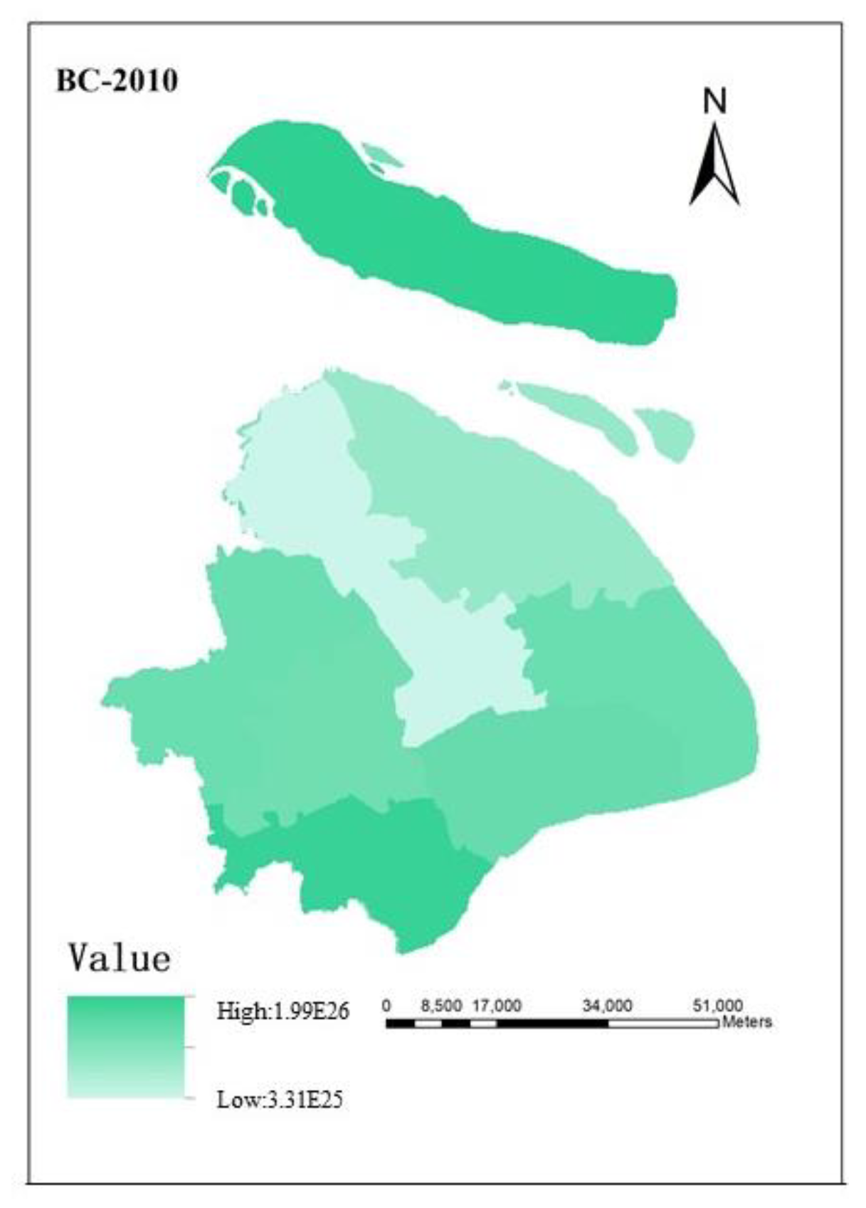
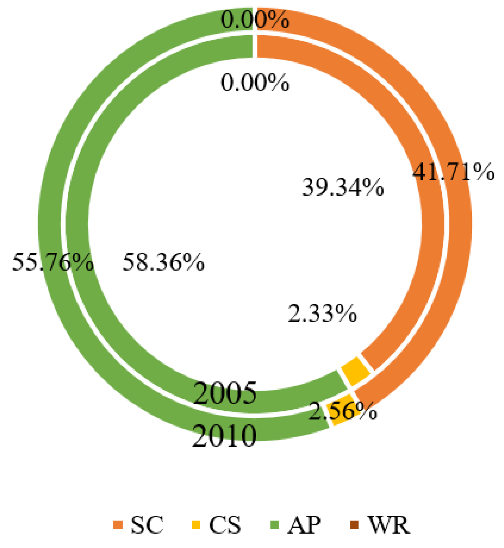
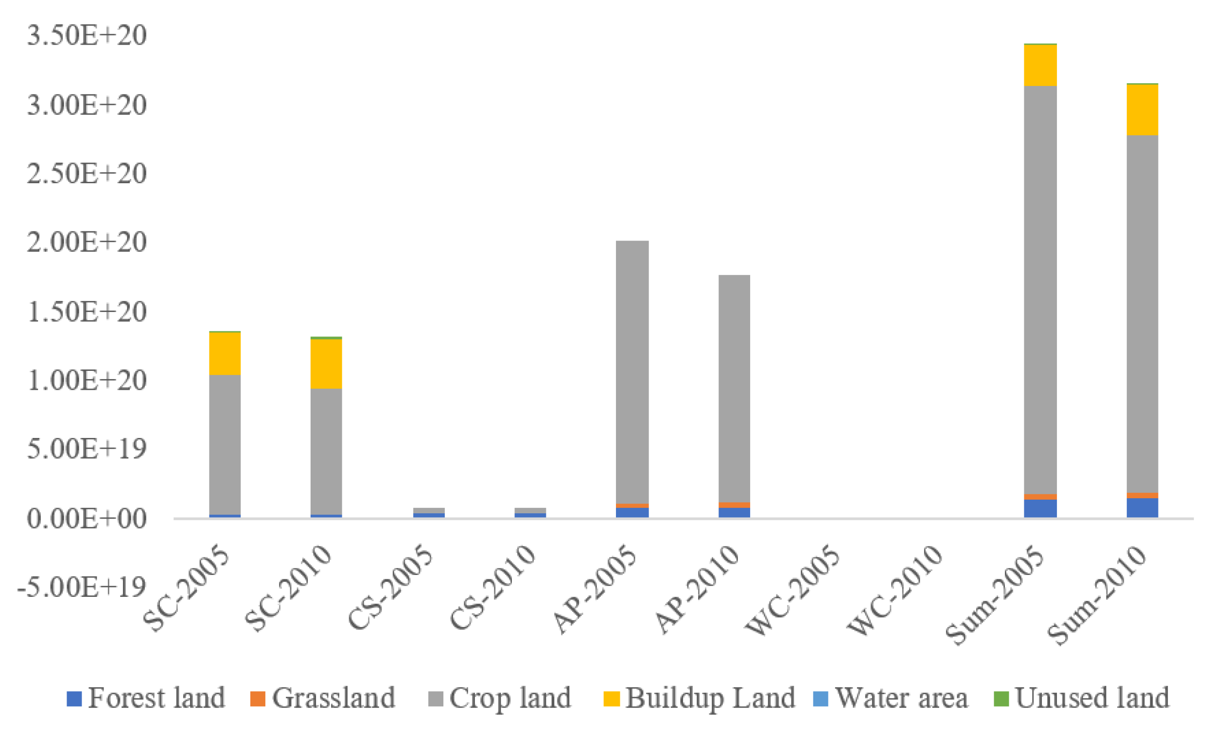
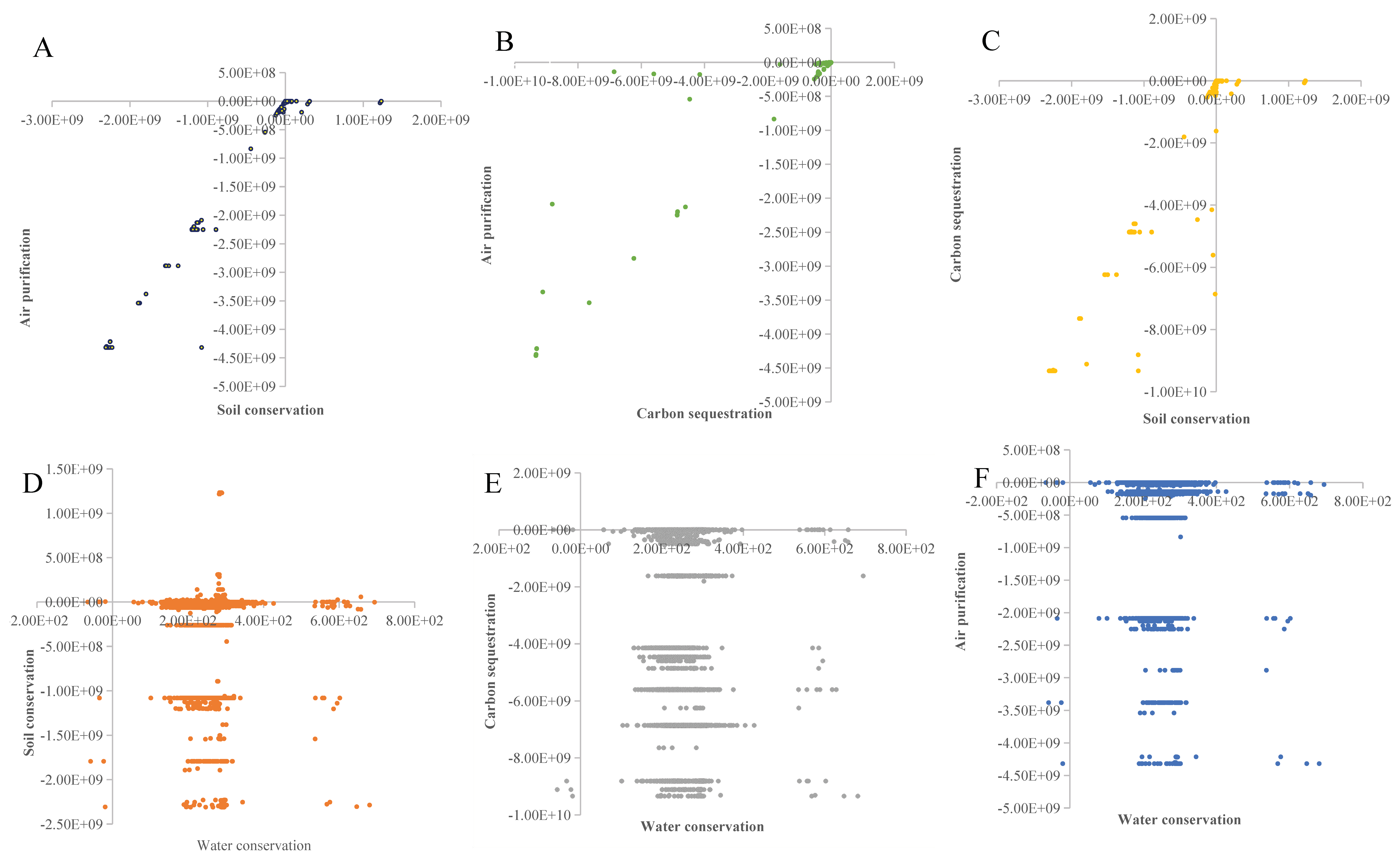
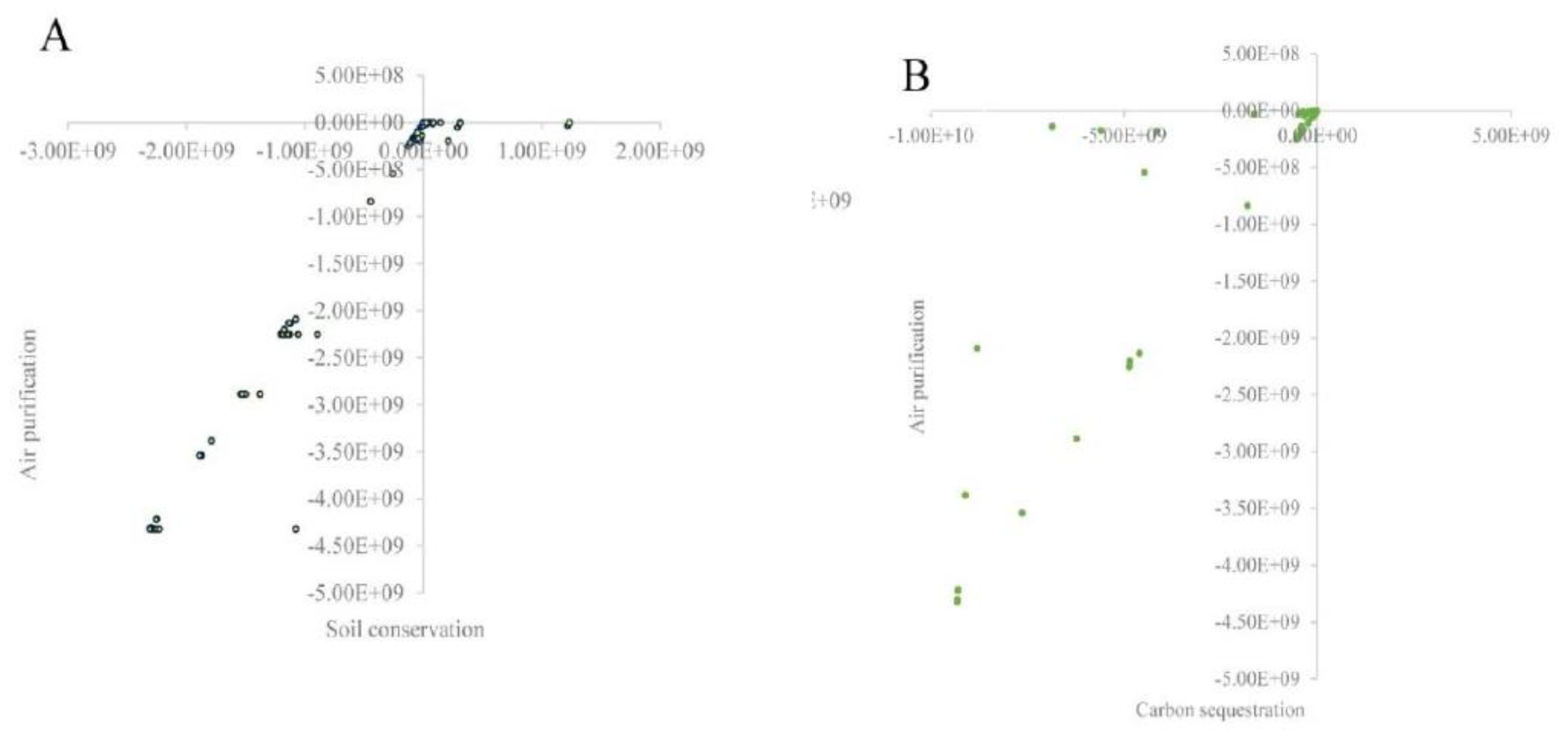
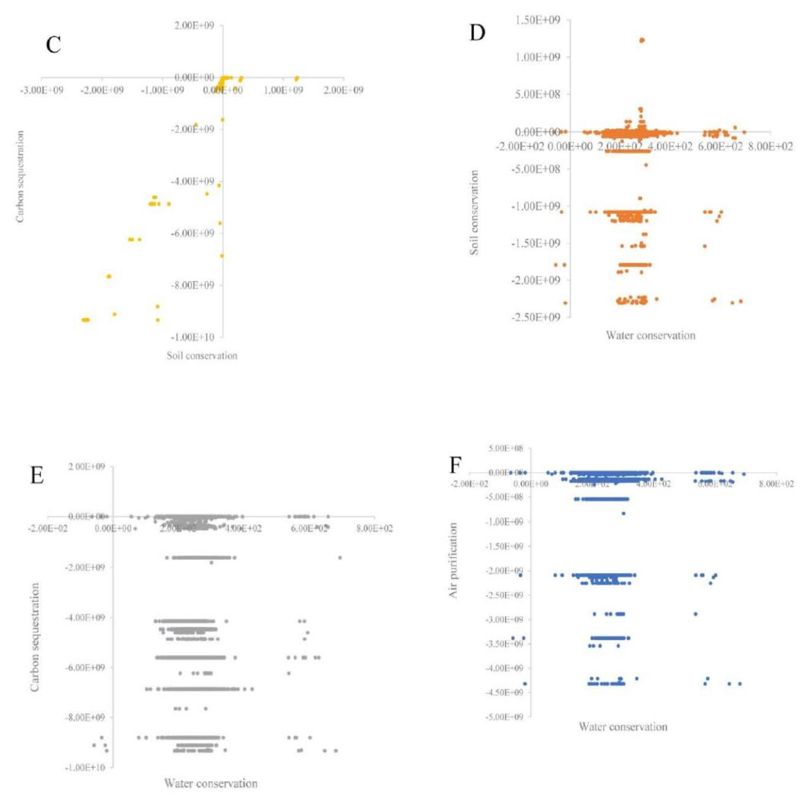
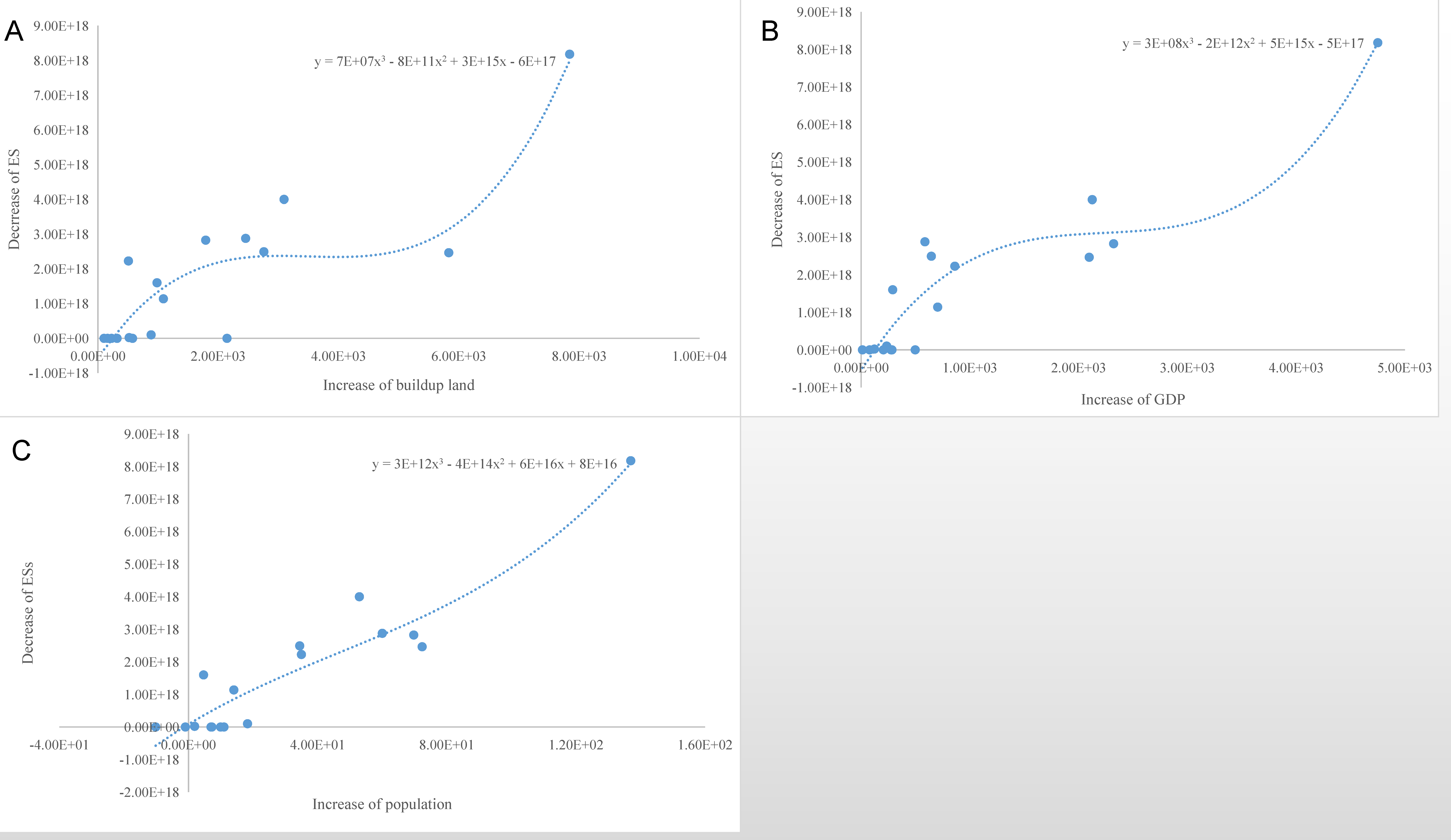
The results reflect that the area of crop land decreased by 10.26% during the study period, while the area of forest land, unused land, and built-up land increased by 4.31%, 36.88%, and 21.72%, respectively. Shanghai’s total ecosystem service value declined by 8.24% from 3.45 × 10²⁰ sej in 2005 to 3.16 × 10²⁰ sej in 2010, mainly contributed by the AP decrease from 2.01 × 10²⁰ sej in 2005 to 1.76 × 10²⁰ sej in 2010. ES of the crop land system contributed the most to the total ES. At the district level, Chongming had the highest value of ES, followed by Pudong and Fengxian. The irregular “U” shape relationships between the decreases of ESs and the increases of urbanization indicators in Shanghai were observed. Synergy relationships among AP, CS, and SC exist, while tradeoff between WR and others can be observed. Finally, most districts experienced the weak decoupling of ESs decrease from urbanization. Results from such a systematic framework can help provide insightful policy implications to move toward sustainable urbanization. To improve the relationships between various ESs and urbanization, we propose the following policy recommendations to the city of Shanghai and other cities facing similar challenges.

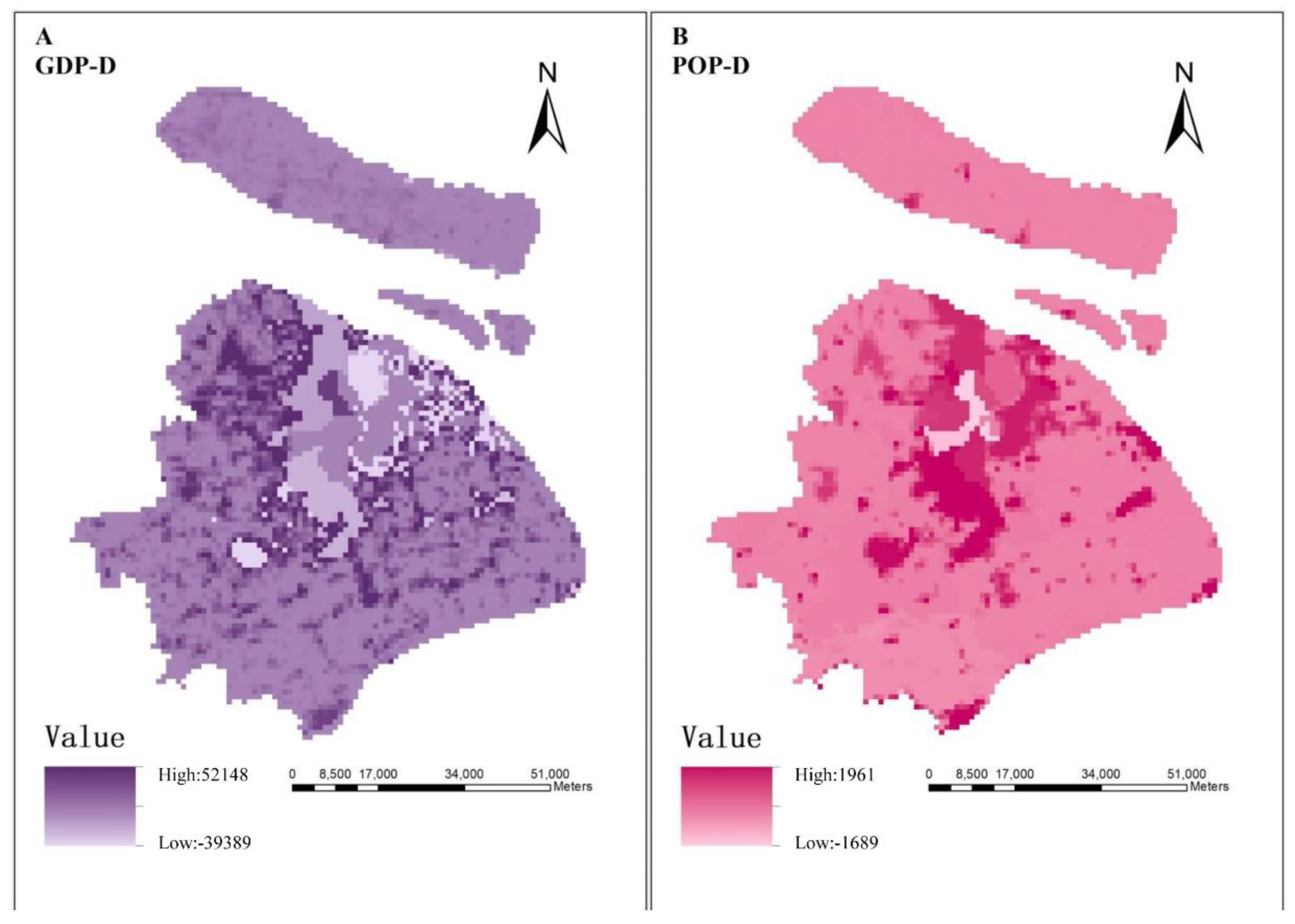
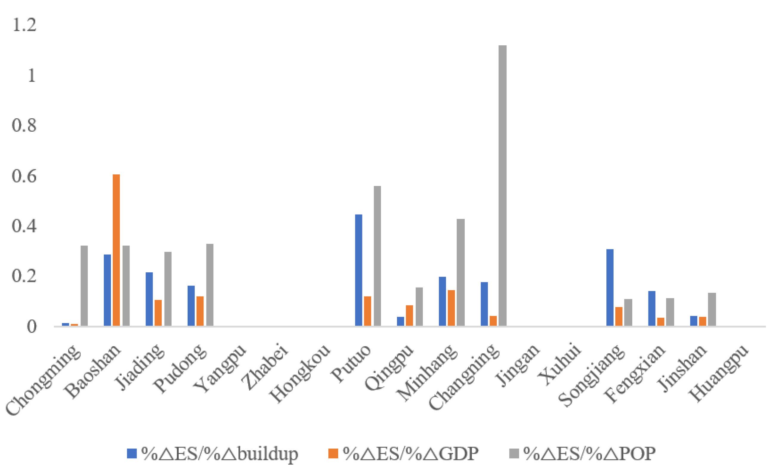
Firstly, urban planners should fully consider all the relevant ES information into their urban plans so that sustainable urban policies can be made. Detailed data should include natural hydrologic and ecological processes, spatial patterns, and dynamic changes of ESs and the synergies and tradeoff relationships among various ESs. For example, our results reflect that the top priority should be given to Chongming and Pudong due to their dominating roles in producing ESs, while Minhang, Jiading, Baoshan, and Pudong also deserve considerable attention due to their decreased ESs during the study period. Spatial heterogeneity in different districts requires more region-specific mitigation policies.

Secondly, a nature-based solution [82] should be carefully employed. Detailed actions include planned ecological redline areas [32], tree-planting campaigns, expanding urban forest and urban parks [83], and the establishment of ecological corridors. Besides, compact use of the built-up land and optimized land planning is effective to overcome the sprawling expansion of the built-up land. Moreover, actions should be taken to compensate for the loss of ESs caused by the crop land decrease.

Finally, it is necessary to adopt this framework to build up an ESs evaluation database covering different regions and cities so that different stakeholders can share related knowledge and information. Such a database can also help decision-makers to dynamically monitor local ecosystems and prepare more appropriate urban policies so that cities can move toward sustainable urban development.

References

1. United Nations. The Sustainable Development Goals Report; United Nations Development Program (UNDP): New York, NY, USA, 2017. [Google Scholar]
2. Seto, K.C.; Guneralp, B.; Hutyra, L.R. Global forecasts of urban expansion to 2030 and direct impacts on biodiversity and carbon pools. Proc. Natl. Acad. Sci. USA 2012, 109, 16083–16088. [Google Scholar] [CrossRef] [PubMed] [Green Version]
3. Fang, C.; Li, G.; Wang, S. Changing and Differentiated Urban Landscape in China: Spatiotemporal Patterns and Driving Forces. Environ. Sci. Technol. 2016, 50, 2217–2227. [Google Scholar] [CrossRef] [PubMed]
4. National Bureau of Statistics of China. China Statistical Yearbook; National Bureau of Statistics of China: Beijing, China, 2018; p. 62791819. Available online: http://www.stats.gov.cn/tjsj/ndsj/2007/indexee.htm (accessed on 9 September 2019).
5. Bai, X.; Shi, P.; Liu, Y. Realizing China’s urban dream. Nature 2014, 509, 158–160. [Google Scholar] [CrossRef] [Green Version]
6. Chen, S.; Chen, B. Changing Urban Carbon Metabolism over Time: Historical Trajectory and Future Pathway. Environ. Sci. Technol. 2017, 51, 7560–7571. [Google Scholar] [CrossRef] [PubMed]
7. Dong, N.; You, L.; Cai, W.; Li, G.; Lin, H. Land use projections in China under global socioeconomic and emission scenarios: Utilizing a scenario-based land-use change assessment framework. Glob. Environ. Chang. 2018, 50, 164–177. [Google Scholar] [CrossRef]
8. MA (Millennium Ecosystem Assessment). Millennium Ecosystem Assessment Synthesis Report; Millennium Ecosystem Assessment: Washington, DC, USA, 2005. [Google Scholar]
9. Costanza, R.; D’Arge, R.; de Groot, R.; Farber, S.; Grasso, M.; Hannon, B.; Limburg, K.; Naeem, S.; O’Neill, R.V.; Paruelo, J.; et al. The value of the world’s ecosystem services and natural capital. Nature 1997, 387, 253–260. [Google Scholar] [CrossRef]
10. Daily, G.D. Nature’s Services: Societal Dependence on Natural Ecosystems; Island Press: Washington, DC, USA, 1997. [Google Scholar]
11. Ouyang, Z.; Zheng, H.; Xiao, Y.; Polasky, S.; Liu, J.; Xu, W.; Wang, Q.; Zhang, L.; Xiao, Y.; Rao, E.; et al. Improvements in ecosystem services from investments in natural capital. Science 2016, 352, 1455–1459. [Google Scholar] [CrossRef]
12. Bukvareva, E.; Zamolodchikov, D.; Grunewald, K. National assessment of ecosystem services in Russia: Methodology and main problems. Sci. Total Environ. 2019, 655, 1181–1196. [Google Scholar] [CrossRef]
13. Luederitz, C.; Brink, E.; Gralla, F.; Hermelingmeier, V.; Meyer, M.; Niven, L.; Panzer, L.; Partelow, S.; Rau, A.L.; Sasaki, R.; et al. A review of urban ecosystem services: Six key challenges for future research. Ecosyst. Serv. 2015, 14, 98–112. [Google Scholar] [CrossRef] [Green Version]
14. Maes, M.J.A.; Jones, K.E.; Toledano, M.B.; Milligan, B. Mapping synergies and trade-offs between urban ecosystems and the sustainable development goals. Environ. Sci. Policy 2019, 93, 181–188. [Google Scholar] [CrossRef]
15. Xi, J. A Report to the 19th National Congress of the Communist Party of China; People’s Publishing House: Beijing, China, 2018. [Google Scholar]
16. Wan, L.; Ye, X.; Lee, J.; Lu, X.; Zheng, L.; Wu, K. Effects of urbanization on ecosystem service values in a mineral resource-based city. Habitat Int. 2015, 46, 54–63. [Google Scholar] [CrossRef]
17. Su, S.; Li, D.; Hu, Y.; Xiao, R.; Zhang, Y. Spatially non-stationary response of ecosystem service value changes to urbanization in Shanghai, China. Ecol. Indic. 2014, 45, 332–339. [Google Scholar] [CrossRef]
18. Zhou, D.; Tian, Y.; Jiang, G. Spatio-temporal investigation of the interactive relationship between urbanization and ecosystem services: Case study of the Jingjinji urban agglomeration, China. Ecol. Indic. 2018, 95, 152–164. [Google Scholar] [CrossRef]
19. Wang, J.; Zhou, W.; Pickett, S.T.A.; Yu, W.; Li, W. A multiscale analysis of urbanization effects on ecosystem services supply in an urban megaregion. Sci. Total Environ. 2019, 662, 824–833. [Google Scholar] [CrossRef]
20. Lyu, R.; Zhang, J.; Xu, M.; Li, J. Impacts of urbanization on ecosystem services and their temporal relations: A case study in Northern Ningxia, China. Land Use Policy 2018, 77, 163–173. [Google Scholar] [CrossRef]
21. Li, B.; Chen, D.; Wu, S.; Zhou, S.; Wang, T.; Chen, H. Spatio-temporal assessment of urbanization impacts on ecosystem services: Case study of Nanjing City, China. Ecol. Indic. 2016, 71, 416–427. [Google Scholar] [CrossRef]
22. Zhan, J.; Zhang, F.; Chu, X.; Liu, W.; Zhang, Y. Ecosystem services assessment based on emergy accounting in Chongming Island, Eastern China. Ecol. Indic. 2018. [Google Scholar] [CrossRef]
23. Tian, L.; Zhao, M.; Peng, J.; Hu, Y.; Wu, J.; Liu, Y. Ecosystem services response to urbanization in metropolitan areas: Thresholds identification. Sci. Total Environ. 2017, 607–608, 706–714. [Google Scholar] [CrossRef]
24. Radford, K.G.; James, P. Changes in the value of ecosystem services along a rural-urban gradient: A case study of Greater Manchester, UK. Landsc. Urban Plan. 2013, 109, 117–127. [Google Scholar] [CrossRef]
25. Song, W.; Deng, X. Effects of urbanization-induced cultivated land loss on ecosystem services in the north China plain. Energies 2015, 8, 5678–5693. [Google Scholar] [CrossRef]
26. Delphin, S.; Escobedo, F.J.; Abd-Elrahman, A.; Cropper, W.P. Urbanization as a land use change driver of forest ecosystem services. Land Use Policy 2016. [CrossRef] [Green Version]
27. Sirakaya, A.; Cliquet, A.; Harris, J. Ecosystem services in cities: Towards the international legal protection of ecosystem services in urban environments. Ecosyst. Serv. 2018, 29, 205–212. [Google Scholar] [CrossRef] [Green Version]
28. Ferreira, L.M.R.; Esteves, L.S.; de Souza, E.P.; dos Santos, C.A.C. Impact of the Urbanisation Process in the Availability of Ecosystem Services in a Tropical Ecotone Area. Ecosystems 2019, 22, 266–282. [Google Scholar]
29. Eigenbrod, F.; Bell, V.A.; Davies, H.N.; Heinemeyer, A.; Armsworth, P.R.; Gaston, K.J. The impact of projected increases in urbanization on ecosystem services. Proc. R. Soc. B Biol. Sci. 2011, 278, 3201–3208. [Google Scholar] [CrossRef] [Green Version]
30. Costanza, R.; de Groot, R.; Sutton, P.; van der Ploeg, S.; Anderson, S.J.; Kubiszewski, I.; Farber, S.; Turner, R.K. Changes in the global value of ecosystem services. Glob. Environ. Chang. 2014, 26, 152–158. [Google Scholar] [CrossRef]
31. Costanza, R.; De Groot, R.; Braat, L.; Kubiszewski, I.; Fioramonti, L.; Sutton, P.; Farber, S.; Grasso, M. Twenty years of ecosystem services: How far have we come and how far do we still need to go? Ecosyst. Serv. 2017, 28, 1–16. [Google Scholar] [CrossRef]
32. Bai, Y.; Wong, C.P.; Jiang, B.; Hughes, A.C.; Wang, M.; Wang, Q. Developing China’s Ecological Redline Policy using ecosystem services assessments for land use planning. Nat. Commun. 2018, 9, 1–13. [Google Scholar] [CrossRef] [Green Version]
33. Zheng, H.; Robinson, B.E.; Liang, Y.-C.; Polasky, S.; Ma, D.-C.; Wang, F.-C.; Ruckelshaus, M.; Ouyang, Z.-Y.; Daily, G.C. Benefits, costs, and livelihood implications of a regional payment for ecosystem service program. Proc. Natl. Acad. Sci. USA 2013, 110, 16681–16686. [Google Scholar] [CrossRef] [Green Version]
34. Sharp, R.; Tallis, H.T.; Ricketts, T.; Guerry, A.D.; Wood, S.A.; Chaplin-Kramer, R.; Nelson, E.; Ennaanay, D.; Wolny, S.; Olwero, N.; et al. InVEST 3.2.0 User’s Guide; The Natural Capital Project, Stanford University, University of Minnesota, The Nature Conservancy, and World Wildlife Fund: Stanford, CA, USA, 2016. [Google Scholar] [CrossRef]
35. Xu, W.; Xiao, Y.; Zhang, J.; Yang, W.; Zhang, L.; Hull, V.; Wang, Z.; Zheng, H.; Liu, J.; Polasky, S.; et al. Strengthening protected areas for biodiversity and ecosystem services in China. Proc. Natl. Acad. Sci. USA 2017, 114, 201620503. [Google Scholar] [CrossRef] [Green Version]
36. Mancini, M.S.; Galli, A.; Coscieme, L.; Niccolucci, V.; Lin, D.; Pulselli, F.M.; Bastianoni, S.; Marchettini, N. Exploring ecosystem services assessment through Ecological Footprint accounting. Ecosyst. Serv. 2018, 30, 228–235. [Google Scholar] [CrossRef]
37. Sun, C.; Wang, Y.; Zou, W. The marine ecosystem services values for China based on the emergy analysis method. Ocean Coast. Manag. 2018, 161, 66–73. [Google Scholar] [CrossRef]
38. Watanabe, M.D.B.; Ortega, E. Dynamic emergy accounting of water and carbon ecosystem services: A model to simulate the impacts of land-use change. Ecol. Model. 2014, 271, 113–131. [Google Scholar] [CrossRef]
39. Odum, H.T. Environmental Accounting: Emergy and Environmental Decision-Making; John Wiley Sons, Inc.: Hoboken, NJ, USA, 1996; Volume 370. [Google Scholar]
40. Pulselli, F.M.; Coscieme, L.; Bastianoni, S. Ecosystem services as a counterpart of emergy flows to ecosystems. Ecol. Model. 2011, 222, 2924–2928. [Google Scholar] [CrossRef]
41. Coscieme, L.; Pulselli, F.M.; Marchettini, N.; Sutton, P.C.; Anderson, S.; Sweeney, S. Emergy and ecosystem services: A national biogeographical assessment. Ecosyst. Serv. 2014, 7, 152–159. [Google Scholar] [CrossRef]
42. Grönlund, E.; Fröling, M.; Carlman, I. Donor values in emergy assessment of ecosystem services. Ecol. Model. 2015, 306, 101–105. [Google Scholar] [CrossRef]
43. Campbell, D.E.; Lu, H.; Walker, H.A. Relationships among the Energy, Emergy, and Money Flows of the United States from 1900 to 2011. Front. Energy Res. 2014, 2. [Google Scholar] [CrossRef] [Green Version]
44. Campbell, E.T.; Tilley, D.R. Valuing ecosystem services from Maryland forests using environmental accounting. Ecosyst. Serv. 2014, 7, 141–151. [Google Scholar] [CrossRef]
45. Lu, H.; Campbell, E.T.; Campbell, D.E.; Wang, C.; Ren, H. Dynamics of ecosystem services provided by subtropical forests in Southeast China during succession as measured by donor and receiver value. Ecosyst. Serv. 2017, 23, 248–258. [Google Scholar] [CrossRef]
46. Yang, Q.; Liu, G.; Casazza, M.; Campbell, E.T.; Giannetti, B.F.; Brown, M.T. Development of a new framework for non-monetary accounting on ecosystem services valuation. Ecosyst. Serv. 2018, 34, 37–54. [Google Scholar] [CrossRef]
47. Zhong, S.; Geng, Y.; Qian, Y.; Chen, W.; Pan, H. Analyzing ecosystem services of freshwater lakes and their driving forces: The case of Erhai Lake, China. Environ. Sci. Pollut. Res. 2019, 26, 10219–10229. [Google Scholar] [CrossRef]
48. Yang, Q.; Liu, G.; Casazza, M.; Hao, Y.; Giannetti, B.F. Emergy-based accounting method for aquatic ecosystem services valuation: A case of China. J. Clean. Prod. 2019. [Google Scholar] [CrossRef]
49. Pan, H.; Geng, Y.; Tian, X.; Wilson, J.; Chen, W.; Zhong, S.; Song, X. Emergy-based environmental accounting of one mining system. Environ. Sci. Pollut. Res. 2019. [Google Scholar] [CrossRef]
50. Mellino, S.; Ripa, M.; Zucaro, A.; Ulgiati, S. An emergy-GIS approach to the evaluation of renewable resource flows: A case study of Campania Region, Italy. Ecol. Model. 2014, 271, 103–112. [Google Scholar] [CrossRef]
51. Pulselli, R.M. Integrating emergy evaluation and geographic information systems for monitoring resource use in the Abruzzo region (Italy). J. Environ. Manag. 2010, 91, 2349–2357. [Google Scholar] [CrossRef]
52. Huang, S.L.; Chen, Y.H.; Kuo, F.Y.; Wang, S.H. Emergy-based evaluation of peri-urban ecosystem services. Ecol. Complex. 2011, 8, 38–50. [Google Scholar] [CrossRef]
53. OECD. Indicators to Measure Decoupling of Environmental Pressure from Economic Growth; OECD Environment Program: Paris, France, 2002. [Google Scholar]
54. Tapio, P. Towards a theory of decoupling: Degrees of decoupling in the EU and the case of road traffic in Finland between 1970 and 2001. Transp. Policy 2005, 12, 137–151. [Google Scholar] [CrossRef] [Green Version]
55. Zhao, X.; Zhang, X.; Li, N.; Shao, S.; Geng, Y. Decoupling economic growth from carbon dioxide emissions in China: A sectoral factor decomposition analysis. J. Clean. Prod. 2017. [Google Scholar] [CrossRef]
56. Lin, B.; Wang, M. Possibilities of decoupling for China’s energy consumption from economic growth: A temporal-spatial analysis. Energy 2019. [Google Scholar] [CrossRef]
57. Chen, J.; Wang, P.; Cui, L.; Huang, S.; Song, M. Decomposition and decoupling analysis of CO2 emissions in OECD. Appl. Energy 2018. [Google Scholar] [CrossRef]
58. Li, Y.N.; Cai, M.; Wu, K.; Wei, J. Decoupling analysis of carbon emission from construction land in Shanghai. J. Clean. Prod. 2019. [Google Scholar] [CrossRef]
59. Lu, Y.; Geng, Y.; Qian, Y.; Han, W.; McDowall, W.; Bleischwitz, R. Changes of human time and land use pattern in one mega city’s urban metabolism: A multi-scale integrated analysis of Shanghai. J. Clean. Prod. 2016, 133, 391–401. [Google Scholar] [CrossRef] [Green Version]
60. Pan, H.; Zhuang, M.; Geng, Y.; Wu, F.; Dong, H. Emergy-based ecological footprint analysis for a mega-city: The dynamic changes of Shanghai. J. Clean. Prod. 2019, 210, 552–562. [Google Scholar] [CrossRef]
61. Yue, W.; Fan, P.; Wei, Y.D.; Qi, J. Economic development, urban expansion, and sustainable development in Shanghai. Stoch. Environ. Res. Risk Assess. 2014, 28, 783–799. [Google Scholar] [CrossRef]
62. Shanghai Statistical Yearbook; China Statistics Press: Beijing, China, 2011. Available online: http://www.stats.gov.cn/tjsj/ndsj/2007/indexee.htm (accessed on 8 September 2019).
63. Liu, G.; Yang, Z. Emergy Theory and Practice: Ecological Environmental Accounting and Urban Green Management; Science Press: Beijing, China, 2018. (in chinese) [Google Scholar]
64. Zhang, W.; Sun, N.; Han, Y. Assessment of atmospheric purification function of urban forest ecosystem in Shanghai. J. Chin. Urban For. 2018, 16, 482–494. [Google Scholar]
65. Teng, H. Assimilating Multi-source Data Model and Map Potential Soil Loss in China. Ph.D. Thesis, Zhejiang University, Hangzhou, China, 2017. [Google Scholar]
66. Brown, M.T.; Ulgiati, S. Emergy assessment of global renewable sources. Ecol. Model. 2016, 339, 148–156. [Google Scholar] [CrossRef] [Green Version]
67. Geng, Y.; Sarkis, J.; Ulgiati, S.; Zhang, P. Measuring China’s circular economy. Science 2013, 340, 1526–1527. [Google Scholar] [CrossRef]
68. Wu, R.; Dai, H.; Geng, Y.; Xie, Y.; Masui, T.; Liu, Z.; Qian, Y. Economic Impacts from PM 2.5 Pollution-Related Health Effects: A Case Study in Shanghai. Environ. Sci. Technol. 2017, 51, 5035–5042. [Google Scholar] [CrossRef]
69. Jia, X.; Fu, B.; Feng, X.; Hou, G.; Liu, Y.; Wang, X. The tradeoff and synergy between ecosystem services in the Grain-for-Green areas in Northern Shaanxi, China. Ecol. Indic. 2014, 43, 103–113. [Google Scholar] [CrossRef]
70. Pan, H.; Zhang, X.; Wu, J.; Zhang, Y.; Lin, L.; Yang, G.; Deng, S.; Li, L.; Yu, X.; Qi, H.; et al. Sustainability evaluation of a steel production system in China based on emergy. J. Clean. Prod. 2016, 112, 1498–1509. [Google Scholar] [CrossRef]
71. Zhang, X.; Jiang, W.; Deng, S.; Peng, K. Emergy evaluation of the sustainability of Chinese steel production during 1998–2004. J. Clean. Prod. 2009, 17, 1030–1038. [Google Scholar] [CrossRef]
72. World Health Organization (WHO). Metrics: Disability Adjusted Life Year (DALY). 2013. Available online: http://www.who.int/healthinfo/global_burden_disease/metrics_daly/en/ (accessed on 6 September 2019).
73. Goedkoop, M.; Spriensma, R. The Eco-indicator 99: A Damage Oriented Method for Life Cycle Impact Assessment: Methodology Report; PRé Sustainability: Amersfoort, The Netherlands, 2000. [Google Scholar]
74. State Forestry Administration of the People’s Republic of China. Specifications for Assessment of Wetland Ecosystem Services; (LY/T2899-2017); State Forestry Administration of the People’s Republic of China: Beijing, China, 2017.
75. Rejani, R.; Rao, K.V.; Osman, M.; Srinivasa Rao, C.; Reddy, K.S.; Chary, G.R.; Pushpanjali, S.J. Spatial and temporal estimation of soil loss for the sustainable management of a wet semi-arid watershed cluster. Environ. Monit. Assess 2016. [Google Scholar] [CrossRef]
76. Kremen, C.; Merenlender, A.M. Landscapes that work for biodiversity and people. Science 2018, 362. [Google Scholar] [CrossRef] [Green Version]
77. Hector, A.; Inchausti, P.; Lavorel, S.; Lawton, J.H.; Lodge, D.M.; Loreau, M.; Naeem, S.; Schmid, B.; Setälä, H.; Symstad, A.J.; et al. Effects of Biodiversity on Ecosystem Functioning: A Consensus of Current Knowledge. Ecol. Monogr. 2005, 75, 3–35. [Google Scholar]
78. Campbell, E.T.; Tilley, D.R. Relationships between renewable emergy storage or flow and biodiversity: A modeling investigation. Ecol. Model. 2016, 340, 134–148. [Google Scholar] [CrossRef]
79. Zheng, H.; Wang, L.; Wu, T. Coordinating ecosystem service trade-offs to achieve win–win outcomes: A review of the approaches. J. Environ. Sci. 2019, 82. [Google Scholar] [CrossRef]
80. Qiu, J.; Turner, M.G. Spatial interactions among ecosystem services in an urbanizing agricultural watershed. Proc. Natl. Acad. Sci. USA 2013, 110, 12149–12154. [Google Scholar] [CrossRef] [Green Version]
81. Zhang, G.; Chen, Y.; Liu, Y.; Zhang, Y.; Liu, Y.; Zhang, Y. On the spatial relationship between ecosystem services and urbanization: A case study in Wuhan, China. Sci. Total Environ. 2018, 637–638, 780–790. [Google Scholar] [CrossRef]
82. Keeler, B.L.; Hamel, P.; McPhearson, T.; Hamann, M.H.; Donahue, M.L.; Meza Prado, K.A.; Arkema, K.K.; Bratman, G.N.; Brauman, K.A.; Finlay, J.C.; et al. Social-ecological and technological factors moderate the value of urban nature. Nat. Sustain. 2019, 2, 29–38. [Google Scholar] [CrossRef]
83. Endreny, T.A. Strategically growing the urban forest will improve our world. Nat. Commun. 2018. [Google Scholar] [CrossRef] [Green Version]
84. Wang, K.C.; Dickinson, R.E.; Wild, M.; Liang, S. Atmospheric impacts on climatic variability of surface incident solar radiation. Atmos. Chem. Phys. 2012, 12, 9581–9592. [Google Scholar] [CrossRef] [Green Version]
85. Sun, P. Land Use Change Analysis and Modeling Prediction in Shanghai Coastal Zone in Recent 30 Years; University of Chinese Academy of Sciences: Beijing, China, 2017. [Google Scholar]
Figure 1. Location of Shanghai and the districts in China [61]. Note that Nanhui district was officially assigned to Pudong New Area on 9 August 2009. Huangpu district and Luwan district were abolished to establish the new Huangpu district in 2011. The State Council approved the withdrawal of Jing’an district and Zhabei district to build a new Jing’an district in November 2015.
Energies 13 06139 g001
Figure 2. Emergy diagram of urban ecosystem services in this study.
Energies 13 06139 g002
Figure 3. The degrees of coupling and decoupling of ESs from urbanization (modified from [54]).
Energies 13 06139 g003
Figure 4. Land use and Land cover (LULC) at district-level. (A): LULC in 2005, (B): LULC in 2010.
Energies 13 06139 g004
Figure 5. Contributions from main districts to land-use change.
Energies 13 06139 g005
Figure 6. Spatial and temporal change of air purification service in Shanghai (sej/yr). (A) spatial distribution of AP in 2005; (B) spatial distribution of AP in 2010; (C) spatial change of AP.
Energies 13 06139 g006
Figure 7. Spatial and temporal change of carbon sequestration service in Shanghai (sej/yr). (A) spatial distribution of CS in 2005; (B) spatial distribution of CS in 2010; (C) spatial change of CS.
Energies 13 06139 g007
Figure 8. Spatial and temporal change of soil conservation service in Shanghai (sej/yr). (A) spatial distribution of SC in 2005; (B) spatial distribution of SC in 2010; (C) spatial change of SC.
Energies 13 06139 g008
Figure 9. Spatial and temporal change of water retention service in Shanghai (sej/yr). (A) spatial distribution of WR in 2005; (B) spatial distribution of WR in 2010; (C) spatial change of WR.
Energies 13 06139 g009
Figure 10. Spatial pattern of biodiversity conservation service of Shanghai in 2010 (sej/yr).
Energies 13 06139 g010
Figure 11. ESs values at the district level in Shanghai (sej/yr). (A): ESs value in 2005 at the district level; (B): ESs value in 2010 at the district level.
Energies 13 06139 g011
Figure 12. Changing trend of total ESs composition in Shanghai.
Energies 13 06139 g012
Figure 13. Changing trend of ecosystem services in Shanghai (sej/yr).
Energies 13 06139 g013
Figure 14. Trade-offs and synergies among the considered ESs at grid scaled level: (A) air purification vs. soil conservation, (B) air purification vs. carbon sequestration, (C) carbon sequestration vs. soil conservation, (D) water retention vs. soil conservation, (E) water retention vs. carbon sequestration, (F) water retention vs. air purification.
Energies 13 06139 g014
Figure 15. Spatial changes in GDP and population from 2010 to 2005 in Shanghai. (A): change of GDP, (B): change of population.
Energies 13 06139 g015
Figure 16. Relationships between the decrease of total ESs and urbanization indicators. (A): built-up land vs. ESs, (B): GDP vs. ESs, (C): population vs. ESs.
Energies 13 06139 g016
Figure 17. Values of urbanization elasticity of ESs at the district-level.
Energies 13 06139 g017