Study on Heat Transfer Performance of Antifreeze-R134a Heat Exchanger (ARHEx)

Abstract

In this paper, the liquid cooling and vapor compression refrigeration system based on an Antifreeze-R134a Heat Exchanger (ARHEx) was applied to the thermal management system for high-power avionics in helicopters. The heat transfer performance of the ARHEx was studied. An experimental prototype of ARHEx was designed and established. A series of experiments was carried out with a ground experimental condition. A heat transfer formula for the antifreeze side in the ARHEx was obtained by means of the coefficient of Nusselt number with experimental analysis. The performance of heat transfer and pressure drop for the refrigerant side of the ARHEx was deduced for the given condition.

1. Introduction

The demand for avionics cooling is increasing with its onboard integration development. In the traditional air-cooling system, the outside ram air compressed by an aircraft engine flows through a series of components, and finally it transfers the waste heat to the outside environment and becomes bleed air [1]. The avionics are cooled by the bleed air, and the heat is brought out. An environment control system (ECS) with air cycle is often used to cool the avionics, but the air bled from the engine decreases the engine performance, and fuel consumption increases [2,3].

Some military helicopters have a large number of high-power airborne electronic equipment that generates a great amount of heat. Both an air cooling system (ACS) and liquid cooling system (LCS) can be used for the cooling of electronic equipment in helicopters. For avionics with low heat flux, the ACS can be used. However, for avionics with high heat flux, there may be many problems when the ACS is adopted. First, the ACS will inevitably bleed an amount of air from the engine, which in turn will result in excessive fuel penalty. Second, excessive air flow cannot be provided by some engines. In addition, it is difficult to arrange the air-cooling pipeline in the electronic equipment cabin due to limited space. Therefore, a new type of helicopter thermal management system should be used to cool the avionics instead of ECS [4].

Based on the above reasons, the vapor compression refrigeration (VCR) system, the LCS, and effective heat transfer have been researched in past years [5,6]. Out of all these cooling systems, the VCR system has a huge advantage because of its high-performance heat transfer and because it is less affected by the external environment. The thermal management system combining the antifreeze liquid cooling (ALC) loop and the VCR loop has been increasingly favored. The ALC loop is composed of an antifreeze tank, pump, Antifreeze-R134a Heat Exchanger (ARHEx), and a high-power electric equipment cold plate, and the VCR loop is composed of a compressor, condenser, electronic expansion valve (EEV), and ARHEx. The compressor and pump provide power for the loop, and the heat can be transferred. When the high-pressure refrigerant liquid condensed by the condenser passes through the EEV, the pressure drops because of the obstruction, which leads to vaporization of the refrigerant liquid. Then, the latent heat of vaporization is absorbed at the same time, so that its temperature is correspondingly reduced, becoming low-temperature and low-pressure vapor. The required cooling capacity can be satisfied by adjusting the speed of the compressor and the opening of the EEV. The antifreeze absorbs a large amount of waste heat discharged from the electronic avionics. Then, its pump forces the antifreeze to pass through its ARHEx, and the waste heat is transferred into the VCR loop. The VCR loop finally discharges the waste heat to the environment. In addition, this system also has high cooling efficiency and stable working characteristics [7,8]. Therefore, many types of aircraft, such as military aircraft F-22 and military helicopter AH-64, NH-90, etc., have adopted this type of thermal management system to remove the waste heat of electronic equipment [9,10].

Although the ARHEx has been used in some types of helicopter, its application is limited. In order to improve its performance in aviation application, a study based on a certain helicopter design should be carried out. In this paper, a series of experiments were carried out to assess the heat transfer performances of an ARHEx. The experimental results under certain experimental conditions were obtained. Based on the experimental analysis, the heat transfer performances were deduced.

2. Helicopter Thermal Management of Avionics Based on ARHEx

2.1. Helicopter Thermal Management System

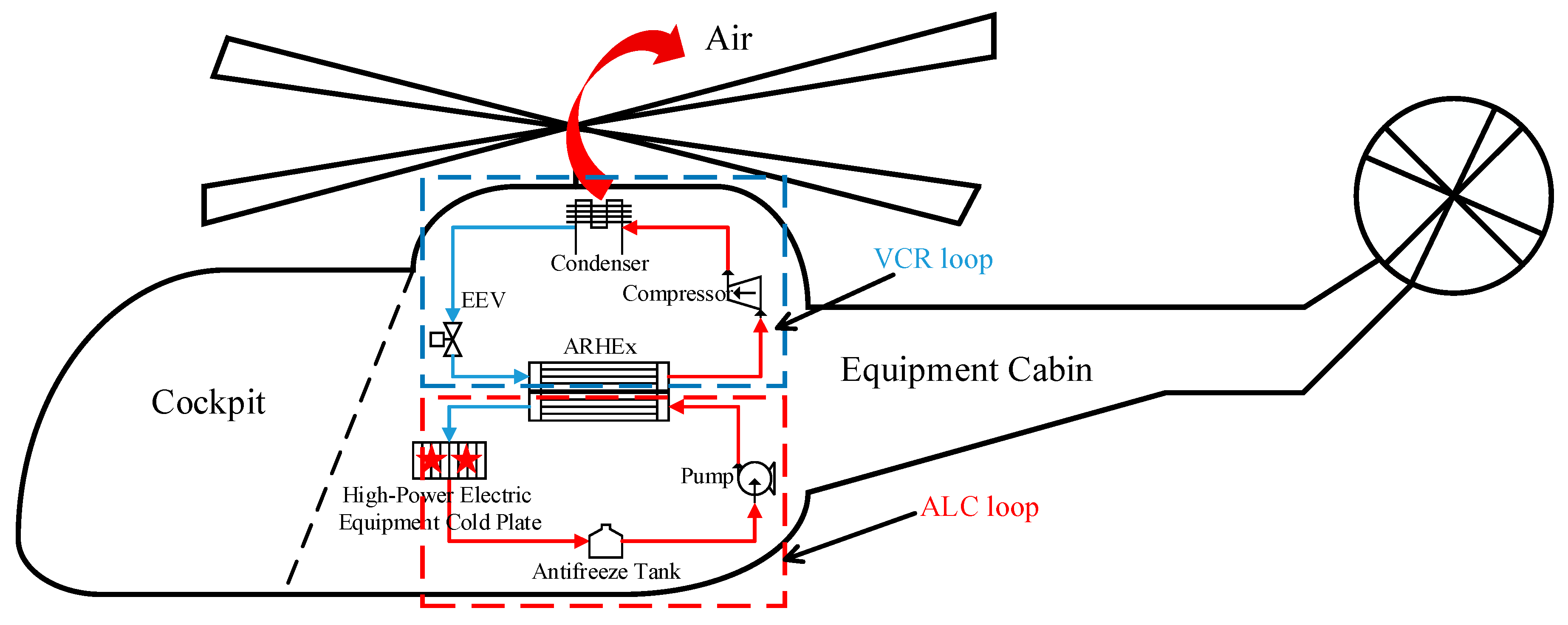
With the increase in heating power of electronic avionics, high-efficiency heat transfer technology has received more attention in recent years. Figure 1 shows the helicopter thermal management system (TMS) for avionics based on a VCR loop and an ALC loop, equipped on the equipment cabin in the helicopter. In the helicopter TMS, its ARHEx is a key component. Its cold side fluid is R134a refrigerant in the VCR loop, and its hot side fluid, or the antifreeze, is 65% glycol aqueous solution. The antifreeze absorbs a large amount of waste heat discharged from the electronic avionics. Then, its pump forces the antifreeze to pass through its ARHEx. In the ARHEx, the antifreeze exchanges heat with the low-temperature refrigerant and transfers the waste heat to the VCR loop. The heated refrigerant finally transfers the waste heat to the outside ram air. In this way, the waste heat in the ALC loop is transferred, and the temperature of the electronic equipment is maintained in a good working range.

Figure 1. Helicopter thermal management system (TMS).

The advantages of this helicopter TMS are as follows: (1) it is less affected by the external flight environment; (2) the varied cooling demands will be met by adjusting the speed of the compressor and the opening of the EEV; (3) the cooling capacity per unit area and heat transfer coefficient of the ARHEx are higher than the evaporator cooled by air.

2.2. Structural Parameters of ARHEx

The heat transfer performance of ARHEx is important for the performance of the helicopter TMS. The ARHEx should be well-designed, otherwise the reliability of electronic avionics cannot be ensured. Hence, it is necessary to test its heat transfer performance.

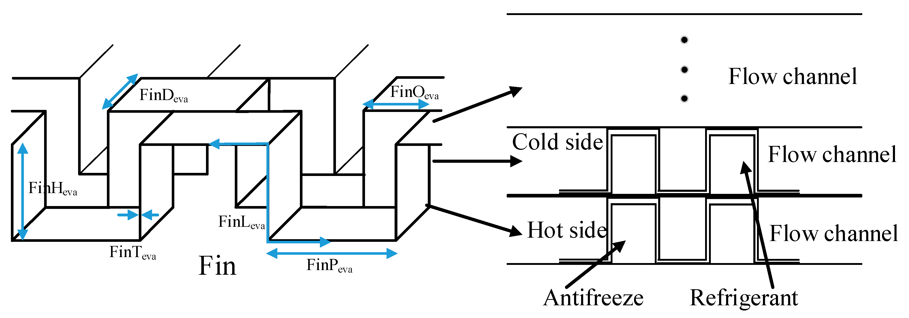
The structure of the studied compact plate fin ARHEx is shown in Figure 2. It is composed of fins and flow channels. The flow channels of antifreeze and refrigerant are arranged alternately. FinP_eva, FinL_eva, FinT_eva, FinH_eva, and FinO_eva represent the fin parameters. In the present study, FinP_eva = 1 mm, FinL_eva = 1 mm, FinT_eva = 0.1 mm, FinH_eva = 1.5 mm, and FinO_eva = 0.5 mm. The height of the flow channel is 1.5 mm. The length, height, and width of the condenser are 270 mm, 160 mm, and 80 mm, respectively. The heat transfer coefficient of ARHEx is increased by arranging the channels to be multi-channel countercurrent. The number of antifreeze and refrigerant channels is 21 and 20, respectively.

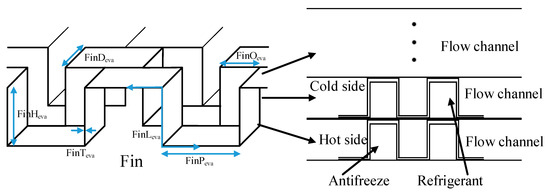
Figure 2. Structure of Antifreeze-R134a Heat Exchanger (ARHEx).

Figure 3 shows the principle of ARHEx. The antifreeze flows into the cylindrical cavity, then flows into the 21 channels, and finally flows out of the ARHEx, while the refrigerant flows into the other 20 channels. The antifreeze and refrigerant exchange heat in the form of cross-flow.

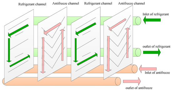
Figure 3. Principle of ARHEx.

3. Experimental Prototype and Experimental Conditions

3.1. Experimental Prototype

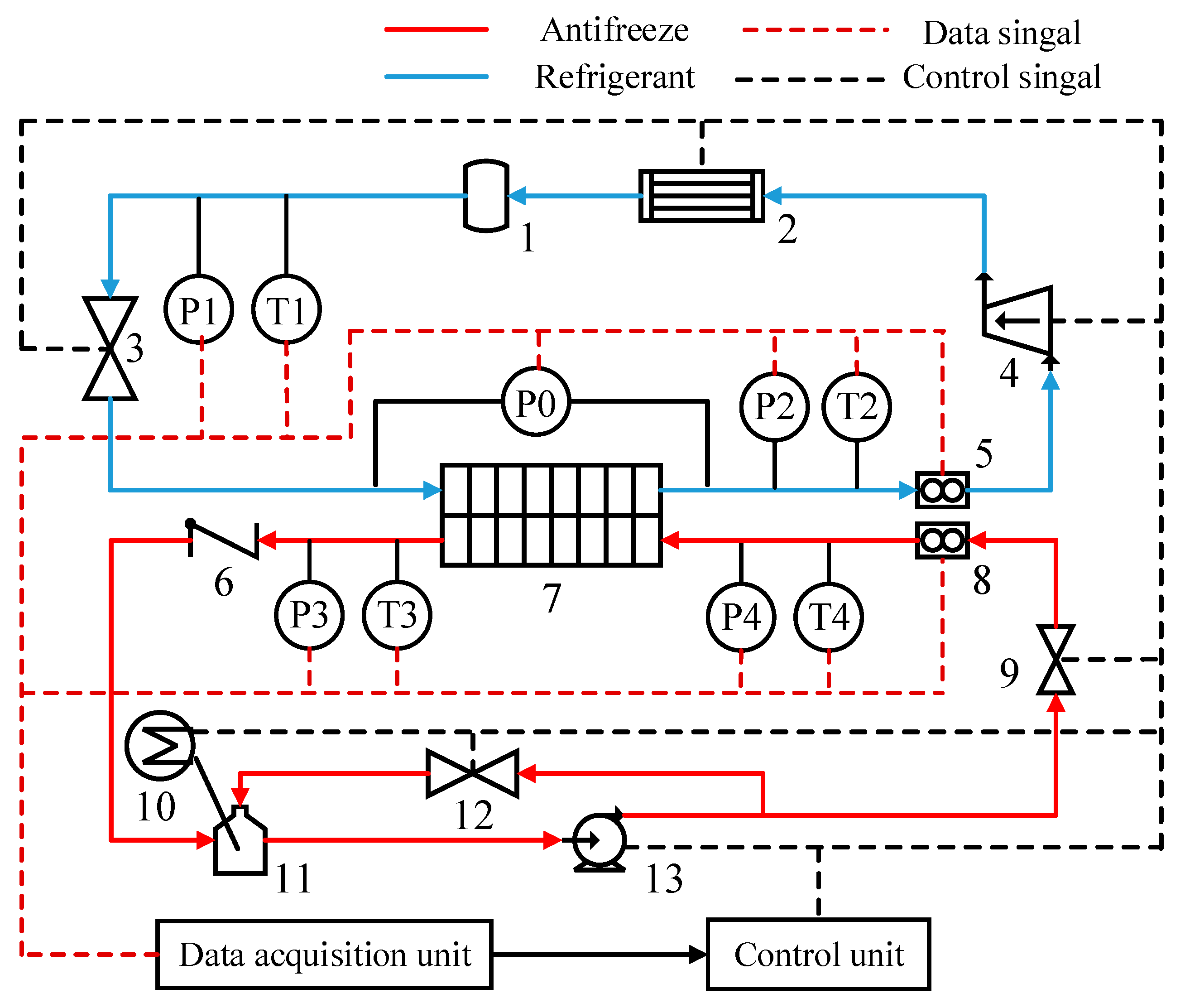
In this study, a high-efficiency heat transfer scheme, which refers to Reference [8], was studied. Figure 4 and Figure 5 present the experimental principle and the experimental device, respectively. It can be seen that the experiment was composed of a VCR loop, an ALC loop, a data acquisition unit, and a control unit.

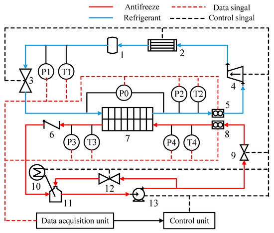
Figure 4. Schematic of the experimental facility [8], (1: condenser dryer; 2: water-cooled plate fin condenser; 3: electronic expansion valve (EEV); 4: compressor; 5: mass flow meter; 6: non-return valve; 7: ARHEx; 8: volume flow meter; 9: control valve; 10: electronic heating device; 11: antifreeze tank; 12: bypass valve; 13: antifreeze pump).

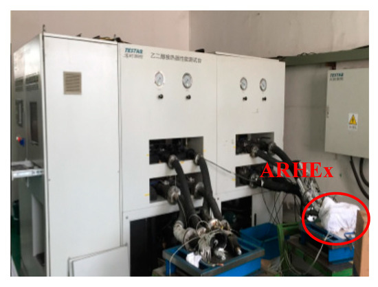
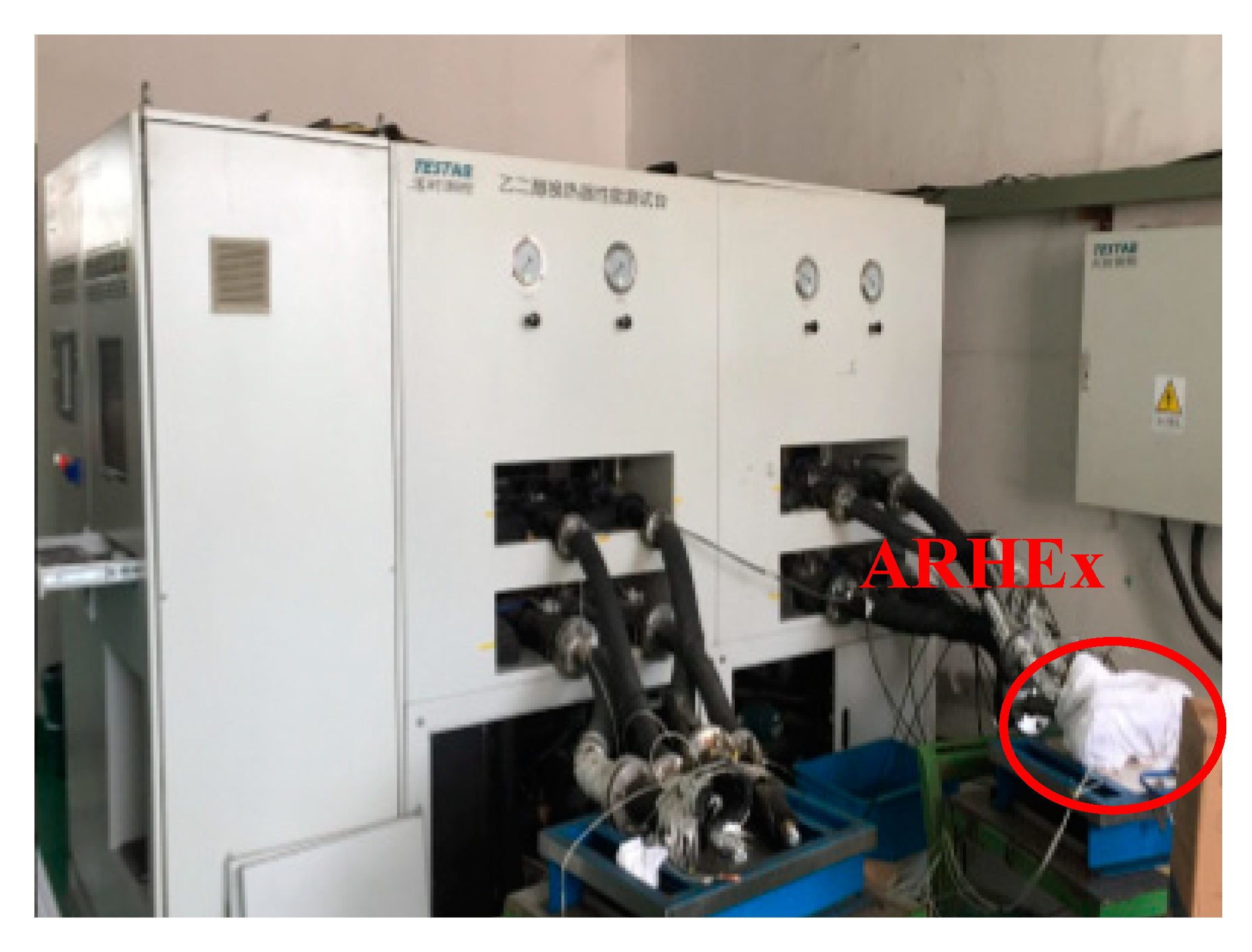
Figure 5. Experimental device.

As shown in Figure 4, the fluid in the VCR loop was R134a, while the fluid in the ALC loop was 65% glycol aqueous solution. In the VCR loop, R134a flowed successively through the ARHEx, mass flow meter, compressor, water-cooled plate fin condenser, condenser dryer, and the EEV. When the vapor compressed by the compressor flowed through the condenser, the heat was dissipated into the ram air, and then the vapor flowed through the EEV with a two-phase state. Finally, the two-phase refrigerant absorbed the heat in the ARHEx, flowed back to the compressor, and achieved a cycle. In the ALC loop, antifreeze flowed successively through the antifreeze tank, antifreeze pump, control valve, ARHEx, and non-return valve. An electric heater was used in our experiment to simulate the heating of electronic avionics.

The mass flow meter was used to measure the value of the refrigerant mass flow rate, and the temperature sensors T1, T2, T3, T4 and the pressure sensors P0, P1, P2, P3, P4 were installed in the appropriate location, as shown in Figure 4; therefore, the temperature or pressure value of the corresponding position was measured. Based on the measured temperature and pressure of the fluid, the enthalpy change value or pressure difference of the corresponding liquid could be calculated.

It should be noted that the uncertainty of the volume flow meter was ±5%, and there were some errors in the use of experimental measurement equipment, so the measurement results needed to be corrected with a data processing method.

The designations related to the position of experimental devices in Figure 4 are listed as follows:

• $\dot{m}$, kg/s, marked with 5, mass flow rate of refrigerant;
• $t_{EEV}^{in}$, °C, marked with T1, inlet temperature of EEV;
• $p_{EEV}^{in}$, kPa, marked with P1, inlet pressure of EEV;
• $t_c^{out}$, °C, marked with T2, refrigerant outlet temperature of ARHEx;
• $p_c^{out}$, kPa, marked with P2, refrigerant outlet pressure of ARHEx;
• ΔP, kPa, marked with P0, refrigerant pressure drop of AREHx;
• ${\dot{V}}_h$, L/min, marked with 8, volume flow rate of antifreeze;
• $t_h^{in}$, °C, marked with T4, antifreeze inlet temperature of ARHEx;
• $p_h^{in}$, kPa, marked with P4, antifreeze inlet pressure of ARHEx;
• $t_h^{out}$, °C, marked with T3, antifreeze outlet temperature of ARHEx;
• $p_h^{out}$, kPa, marked with P3, antifreeze outlet pressure of ARHEx.

To minimize the leaking heat, the ARHEx and the connected pipes had to be wrapped with polyurethane foam and aluminum foil, as shown in Figure 5.

The experiment was designed to study the heat transfer performance of the ARHEx. The experimental data were not recorded until the system worked steadily. The flow rates, pressure, and temperature of the fluids were monitored and then used in the subsequent calculation and analysis. It is noted that the measurement data were not recorded until the system stabilized for 25 min.

3.2. Experimental Conditions

In the ground experimental tests, the low-temperature refrigerant flowed into the cold side of ARHEx, and the high-temperature antifreeze flowed into the hot side of ARHEx. According to the design requirements of the experiments, the superheat, SH, was required as the calculated parameter. SH of the refrigerant at the ARHEx outlet is expressed as

$$SH=t_c^{out}-t_{eva}$$

(1)

where $t_c^{out}$ is the refrigerant outlet temperature of the ARHEx obtained by resistance thermometers marked with T2, °C; t_eva is the evaporation temperature, °C, and is uniquely determined by $p_c^{out}$.

The unknown properties were calculated using the REFPROP software in this study. Assuming the flow process in the EEV is an adiabatic expansion process, the refrigerant enthalpy at the ARHEx inlet, $H_c^{in}$, is defined as

$$H_c^{in} \approx H_{EEV}^{in}$$

(2)

where $H_{EEV}^{in}$ indicates the inlet refrigerant enthalpy of EEV, kJ/kg, and can be calculated with $t_{EEV}^{in}$ and $p_{EEV}^{in}$.

Meanwhile, the refrigerant enthalpy at the ARHEx outlet, $H_c^{out}$, can be calculated by $t_c^{out}$ and $p_c^{out}$.

The pressure of the refrigerant at the ARHEx inlet is expressed as

$$p_c^{in}=\mathsf{\Delta }P+p_c^{out}$$

(3)

where $p_c^{in}$ is the inlet pressure of the ARHEx, kPa; ΔP is the refrigerant pressure drop of the ARHEx, kPa;$p_c^{out}$ is the outlet pressure of the ARHEx, kPa.

Based on $H_c^{in}$ and $p_c^{in}$, the thermodynamic state of refrigerant at the ARHEx inlet could be obtained.

The heating powers of the electronic equipment were 5, 8, 10, 12, and 15 kW, respectively. In this study, $p_c^{out}$, ${\dot{V}}_h$, and $t_h^{in}$ could be regulated. However, they were not adjusted together. The experimental conditions are shown in Table 1.

Table 1. Experimental conditions.

No.	Symbol	Parameter	Value	Unit
1	$t_{EEV}^{in}$	Inlet temperature of EEV	50	°C
2	$p_{EEV}^{in}$	Inlet pressure of EEV	1492	kPa
3	$p_c^{out}$	Outlet pressure on refrigerant side	338, 362, 388, 415	kPa
4	SH	Outlet superheat on refrigerant side	5	°C
5	${\dot{V}}_h$	Antifreeze volume flow	20, 35, 50, 60	L/min
6	$t_h^{in}$	Inlet temperature on antifreeze side	20, 25, 30, 35, 40	°C
7	$p_h^{out}$	Outlet pressure on antifreeze side	100	kPa

3.3. Experimental Stability

Based on the basic heat transfer calculations, for a group of setting experimental data, heat transfer quantity for antifreeze and refrigerant are defined, respectively.

The heat transfer quantity for the antifreeze can be calculated by Equation (4) [11]:

$$Q_A=Cp\cdot {\stackrel{·}{V}}_h\cdot \rho \cdot \left(t_h^{in}-t_h^{out}\right).$$

(4)

where Q_A is the heat transfer quantity for the antifreeze, kW; Cp is the antifreeze specific heat capacity, J/(kg·°C); ρ is the antifreeze density, kg/m³; ${\dot{V}}_h$ is the volume flow rate of antifreeze, L/min;$t_h^{in}$ is the antifreeze inlet temperature of ARHEx, °C;$t_h^{out}$ is the antifreeze outlet temperature of ARHEx, °C.

The heat transfer quantity for the refrigerant is as follows:

$$Q_R^{\prime }=\stackrel{·}{m}\cdot \left(H_c^{out} - H_c^{in}\right)$$

(5)

where $Q_R^{\prime }$ is the heat transfer quantity for the refrigerant, kW; $\dot{m}$ is the mass flow rate of refrigerant, kg/s; $H_c^{in}$ is the inlet refrigerant enthalpy of ARHEx, kJ/kg; $H_c^{out}$ is the outlet refrigerant enthalpy of ARHEx, kJ/kg.

For each experimental condition, the unsteadiness can be calculated using Equation (6) [12]:

$${\mathsf{\Delta }}_Q=\frac{\sqrt{{\left(Q_A-Q_m\right)}^2+{\left(Q_R-Q_m\right)}^2}}{Q_m}$$

(6)

and

$$Q_m=\frac{Q_A+Q_R}{2}$$

(7)

where ∆_Q is the unsteadiness; Q_m is mean value of heat transfer quantity, kW.

Hence, the heat transfer quantity of ARHEx is expressed as $Q_m\cdot \left(1\pm {\mathsf{\Delta }}_Q\right)$. In engineering practice, it is acceptable that the heat balance dispersion or unsteadiness is in the range of 3–7% [11,12,13,14,15]. We have adopted Δ_Q < 6% as a criterion in our analysis.

In this study, the measurement data were modified with the least-squares method; the accuracy of measurement sensors was corrected. Suppose that the data measured by the standard sensors is y, and the data measured by the experimental sensors is x. Then the data can be corrected by the following linear fitting formula:

$$y=\widehat{a}x+\widehat{b}$$

(8)

By measuring a series of different values, $\widehat{a}$ and $\widehat{b}$ can be calculated by the following formula:

$$\{\begin{array}{c}\widehat{a}=\left({\displaystyle \sum _{i=1}^{n}xy-n\overline{x}\overline{y}}\right)/\left({\displaystyle \sum _{i=1}^n{x}^2-n{\left(\overline{x}\right)}^2}\right)\\ \widehat{b}=\overline{y}-\widehat{a}\overline{x}\hfill \end{array}$$

(9)

4. Experimental Result Analysis

4.1. Heat Transfer Quantity

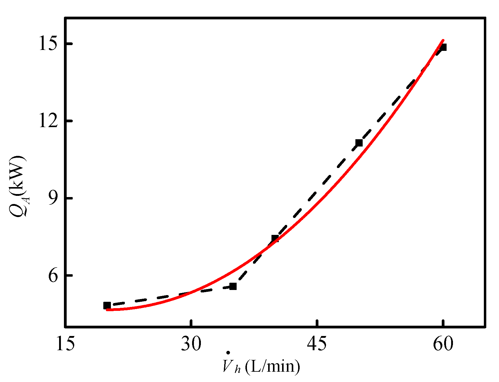
In the heat exchanger experiments, the antifreeze volume flow rate, ${\dot{V}}_h$, could be regulated, and the remaining two variables remained constant, namely, $t_h^{in}$= 30 °C and $p_c^{out}$ = 338 kPa.

Figure 6 shows the relationship of Q_A and ${\dot{V}}_h$ for the given conditions, where Q_A is calculated with Equation (4). In Figure 6, the dotted line is the experimental data, and the solid line is the fitting curve. With the increase in volume flow rate, the heat transfer quantity obviously increases. When the volume flow reaches 60 L/min, the heat transfer quantity is 15 kW.

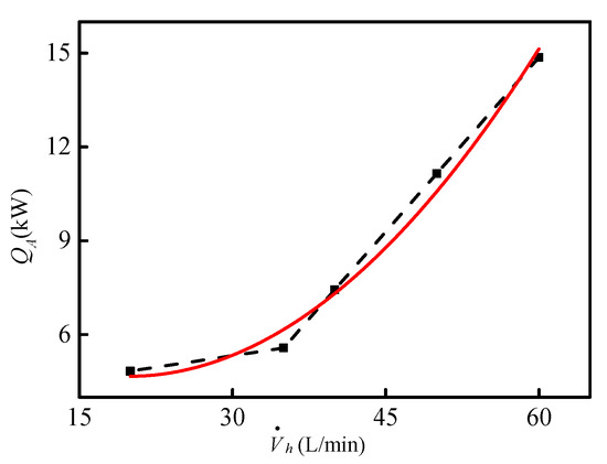
Figure 6. Relationship of Q_A and ${\dot{V}}_h$.

4.2. Efficiency of Heat Transfer

The efficiency of heat transfer is calculated by Equation (8) [2,10]:

$${\eta }_0=\frac{t_h^{in}-t_h^{out}}{t_h^{in}-t_c^{out}}$$

(10)

where ${\eta }_0$ is the efficiency of heat transfer, %; $t_h^{in}$ is the inlet temperature of the hot side antifreeze, °C; $t_h^{out}$ is the outlet temperature of the hot side antifreeze, °C; $t_c^{out}$ is the outlet temperature of the cold side refrigerant, °C.

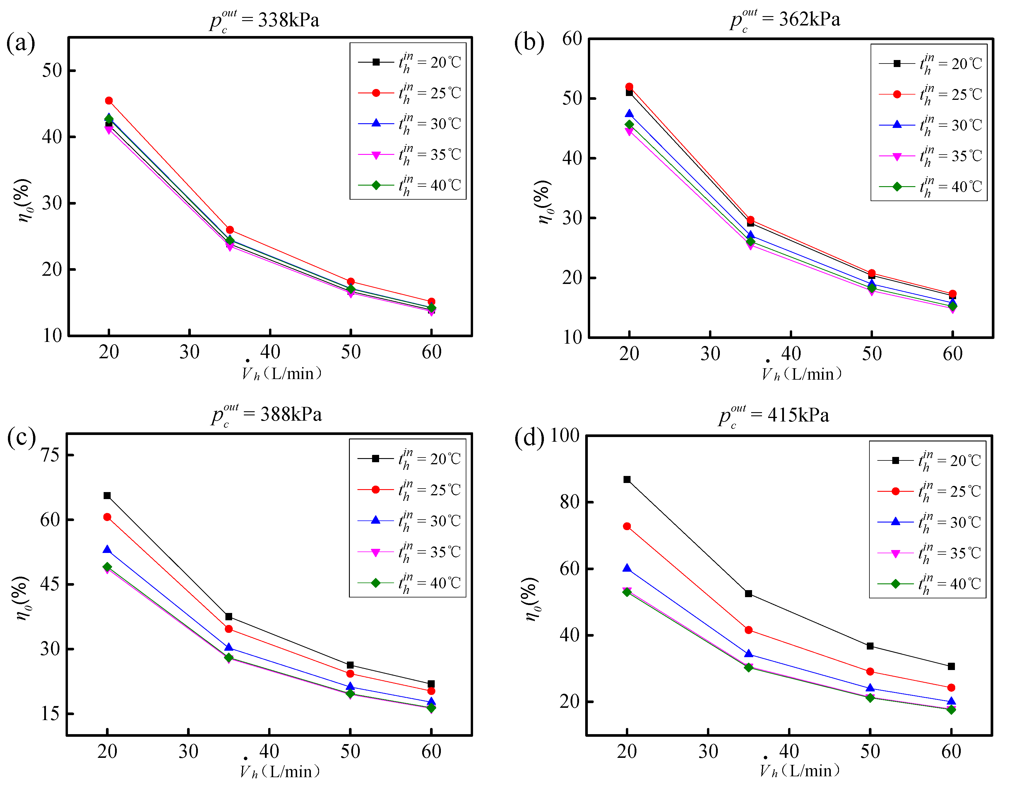
In the experiment, a constant inlet enthalpy, $H_c^{in}$, and a constant outlet superheat, SH, were kept for the cold side refrigerant. The inlet volume flow, ${\dot{V}}_h$, and the temperature of the hot side antifreeze, $t_h^{in}$, were changed. The calculation relationship of η₀ = f ($p_c^{out},t_h^{in},t_c^{in}$) could be obtained. More than 80 experiments were carried out to obtain this relationship. In these ground experiments, $H_c^{in}$ ≈ 271.52 kJ/kg, SH ≈ 5 °C, and ${\dot{V}}_h$ was controlled at 20, 35, 50, and 60 L/min, respectively. $t_h^{in}$ and $p_c^{out}$ were varied, respectively. Figure 7a–d shows the relationship of η₀ and $p_c^{out}$ for the given values of $t_h^{in}$ and ${\dot{V}}_h$.

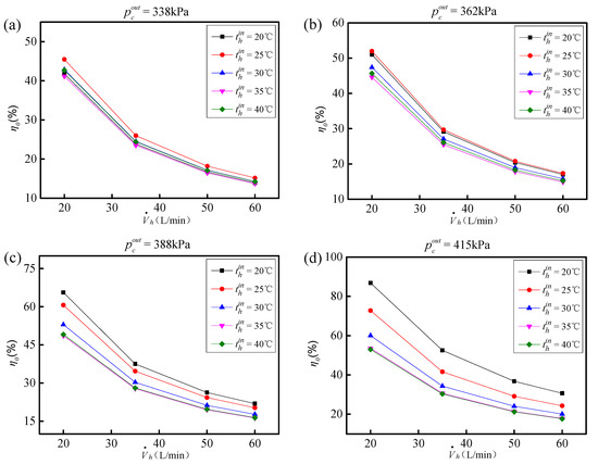
Figure 7. Relationship of η₀ and $p_c^{out}$ for given $t_h^{in}$ and $t_c^{in}$.

From Figure 7, some conclusions can be observed when $p_c^{out}$ varies from 338 kPa to 415 kPa:

(1)

With the increase of ${\dot{V}}_h$, η₀ decreases gradually. For $p_c^{out}$ = 338 kPa and $p_c^{out}$ = 362 kPa under the same volume flow rate, η₀ does not necessarily decrease with the increase of $t_h^{in}$. However, for $p_c^{out}$ = 388 kPa and $p_c^{out}$ = 415 kPa under the same volume flow rate, η₀ decreases with the increase of $t_h^{in}$.

(2)

η₀ increases gradually with the increase of $p_c^{out}$. For all experimental results, when $p_c^{out}$ = 415 kPa, $t_h^{in}$ = 20 °C and ${\dot{V}}_h$ = 20 L/min, η₀ reaches its maximum value and is 86%. When $p_c^{out}$ = 338 kPa, $t_h^{in}$ = 40 °C and ${\dot{V}}_h$ = 60 L/min, η₀ reaches its minimum value and is 16%.

Figure 8 shows the relationship of η₀ = f ($p_c^{out},t_h^{in},t_c^{in}$). In Figure 8, letters A, B, C, and D indicate that $p_c^{out}$ is equal to 415, 388, 362, and 338 kPa, respectively. The relationship between η₀ and $p_c^{out},t_h^{in}$ and $t_c^{in}$ is clear.

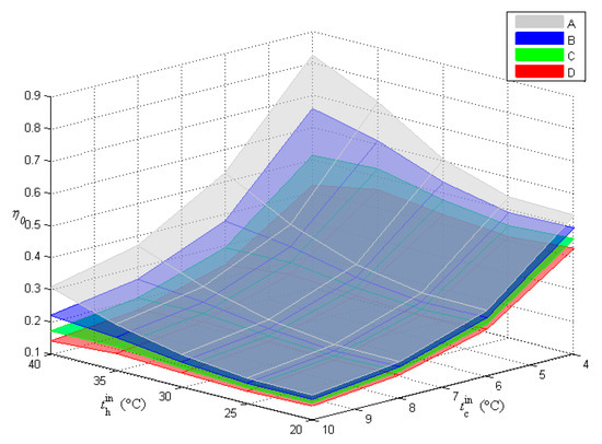
Figure 8. Relationship of η₀ = f ($p_c^{out},t_h^{in},t_c^{in}$).

4.3. Heat Transfer Formula for Antifreeze

On the basis of the experiments, the heat transfer formula of the antifreeze in the ARHEx can be deduced, and then the convective heat transfer coefficients can be calculated.

The heat transfer between the antifreeze and the wall of the ARHEx can be calculated as follows (9) [11,12,13]:

$$Q_A=h_{eva,A}\cdot A_{\mathrm{eva},A}\cdot \left(T_{eva,A}-T_{eva,wall}\right)$$

(11)

where h_eva,A is the heat transfer coefficient, W/(m²·°C); A_eva,A is the heat transfer area, m². T_eva,A is the mean value of antifreeze temperature, T_eva,A = ($t_h^{in}$ +$t_h^{out}$)/2, °C; T_eva,wall is the wall temperature, °C.

The heat transfer coefficient is as follows:

$$h_{eva,A}=\frac{{\mathrm{Nu}}_A\cdot {\lambda }_A}{D_A}$$

(12)

The Nusselt number of antifreeze side is calculated by the following formula [14,15,16,17,18,19]:

$${\mathrm{Nu}}_A=a\cdot {\mathrm{Re}}^b\cdot {\mathrm{Pr}}^c$$

(13)

and

$$\mathrm{Re}=\frac{\rho \cdot v\cdot D_A}{\mu },\dots \mathrm{Pr} = \frac{\mu \cdot Cp}{{\lambda }_A}$$

(14)

where Nu_A is the Nusselt number; Re is the Reynolds number; Pr is the Prandtl number; a is correction coefficient considering various factors; b is experience index; c is a constant value, 0.4; ρ is antifreeze density, kg/m³; v is the antifreeze velocity, m/s; D_A is the antifreeze hydraulic diameter, m; Cp is the antifreeze specific heat capacity, J/(kg·°C); μ is the antifreeze dynamic viscosity, Pa·s; λ_A is the thermal conductivity of antifreeze, W/(m·°C).

The calculated values of Nu_A are plotted against various Re and are shown in Figure 9. With 80 experimental results, regression analysis has been used to fit, and the regression resulted in the following:

$${\mathrm{Nu}}_A=0.5\cdot {\mathrm{Re}}^{1.396}\cdot {\mathrm{Pr}}^{0.4}$$

(15)

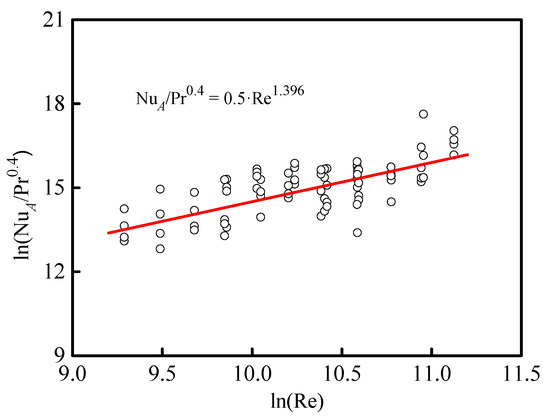
Figure 9. Plot of ln(Nu_A/Pr^0.4) as a function of ln(Re) for the experimental data.

4.4. Heat Transfer and Pressure Drop Formula for Refrigerant

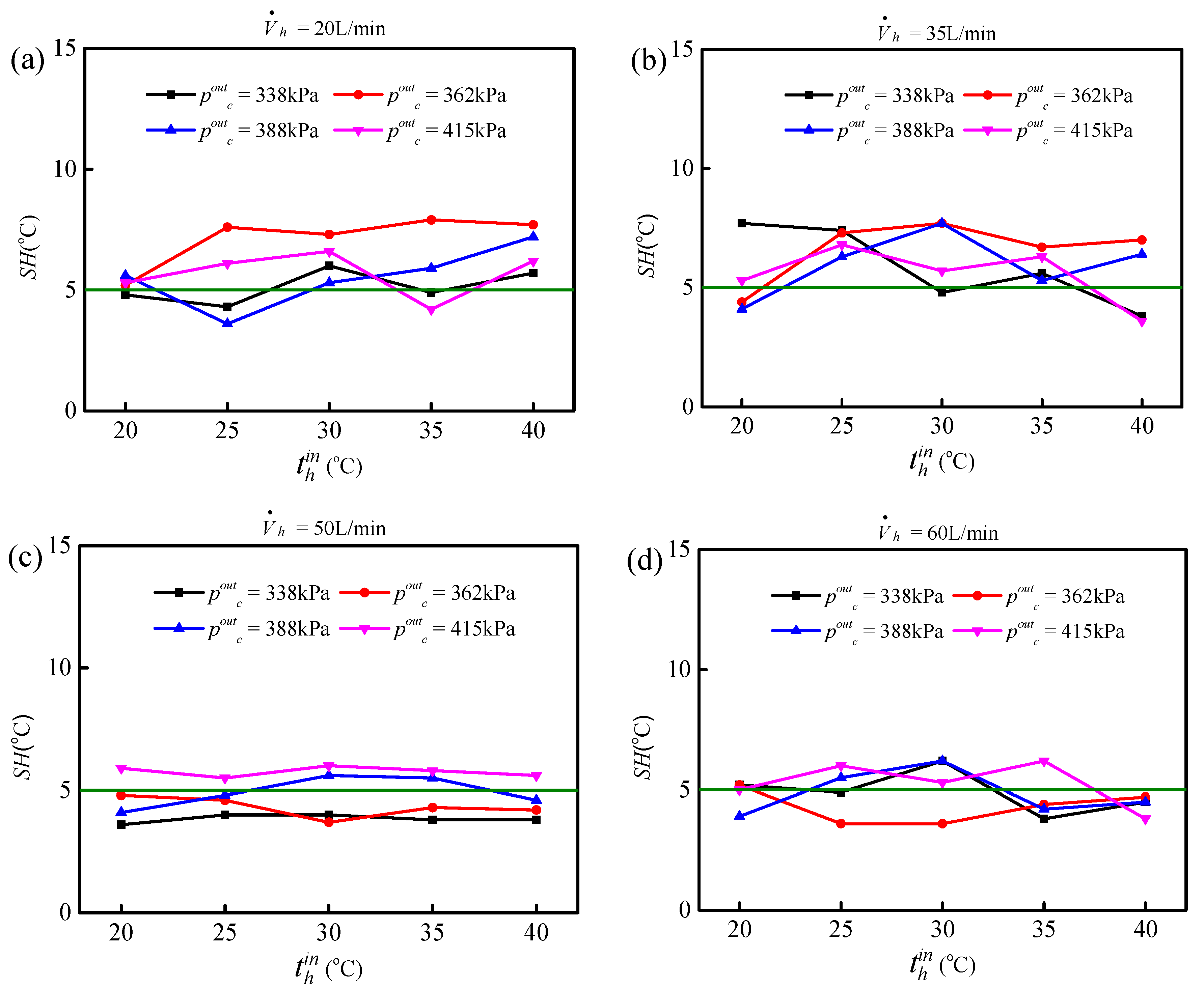
In our 80 experiments, refrigeration was subcooled by a circulation of cold water in the condenser. It became two-phase fluid with 0.3–0.35 dryness by the EEV. Then it became slightly superheated vapor after it flowed through the ARHEx.

In this experiment, the SH was about 5 °C. However, there was always the deviation of $t_c^{out}$ in the actual experiment, which made the SH distribute around 5 °C. Figure 10a–d shows the SH during the actual experimental process.

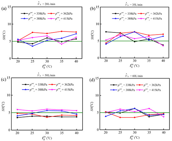
Figure 10. Relationship of SH for given $t_h^{in}$ and $p_c^{out}$.

In the refrigerant side, the heat transfer between the refrigerant and the wall of heat exchanger can be calculated by Equation (14) [20,21].

$$Q_R=h_{eva,R}\cdot A_{\mathrm{eva},\mathrm{R}}\cdot \left(t_{eva}-T_{eva,wall}\right)$$

(16)

where Q_R is the heat transfer quantity, W; h_eva,R is the convective heat transfer coefficient between the refrigerant and the wall, W/(m²·°C); A_eva,R is the heat transfer area, m²; t_eva is the refrigerant evaporation temperature, °C; T_eva,wall is the wall temperature, °C.

Gnielinski correlation is used to calculate the convective heat transfer coefficient as follows [22,23,24]:

$$h_{eva,R}=\sqrt[3]{h_{cv}^3+h_{NcB}^3},$$

(17)

$$h_{cv}=h_{LO}·F_{TP},$$

(18)

$$h_{LO}=\frac{\left(\xi /8\right)·(\mathrm{Re}-1000)\cdot \mathrm{Pr}}{1+12.7\cdot (\xi /8{)}^{0.5}\cdot ({\mathrm{Pr}}^{2/3-1.0})}·\frac{{\lambda }_R}{D_R}.$$

(19)

where h_NcB is the nucleate boiling contribution, W/(m²·°C); F_TP is the correlation coefficient; ξ is the friction factor coefficient; D_R is the hydraulic diameter in cold side, m; λ_R is the thermal conductivity of refrigerant, W/(m·°C); Re is the Reynolds number; Pr is the Prandtl number.

The pressure drop on the refrigeration side consists of three parts [25]: the friction pressure drop, the acceleration pressure drop due to a change in the fluid density along the flow axis, and the pressure drop due to gravity. Compared with the other two pressure drop components, the friction pressure drop has a large proportion. Hence, the other two pressure drops are ignored, and the pressure drop of cold side refrigerant is calculated by the following formulas [26,27,28]:

$$\mathsf{\Delta }P \approx {\left(\frac{dP}{dz}\right)}_F=k_{dp}\frac{\xi ·G^2·\overline{v}}{2D_R},G=A_R\cdot \stackrel{·}{m}$$

(20)

$$\xi =8{\left[{\left(\frac{8}{\mathrm{Re}}\right)}^{12}+{\left({\left[2.457\ln \left({\left(\frac{7}{\mathrm{Re}}\right)}^{0.9}+0.27\left({\frac{\epsilon }{D}}_R\right)\right)\right]}^{16}+{\left[\frac{37530}{\mathrm{Re}}\right]}^{16}\right)}^{-3/2}\right]}^{1/12}$$

(21)

where k_dp is the pressure drop gain coefficient; A_R is the cross-area of refrigerant side, m²;$\dot{m}$ is the refrigerant mass flow rate, kg/s; $\overline{v}$ is refrigerant flow velocity, m/s; ε is the absolute roughness; D_R is the hydraulic diameter of refrigerant side, m.

In the Equation (16), h_eva,R is the heat exchange coefficient computed from the heat exchange correlations without any modifications, so the heat transfer quantity Q_R computed with the experimental temperature data also needed to be modified. The equation can be established as follows:

$$Q_A=k_{eva,R}·Q_R=Cp·{\dot{V}}_h·\rho ·\left(t_h^{in}-t_h^{out}\right)$$

(22)

where k_eva,R is the heat transfer gain coefficient. k_eva,R and k_dp in the heat transfer and pressure drop formulas of the refrigerant side can be deduced using the experimental data. Figure 11 shows the fitting result of heat transfer gain coefficient, and k_eva,R = 8. In the same way, k_dp = 1.

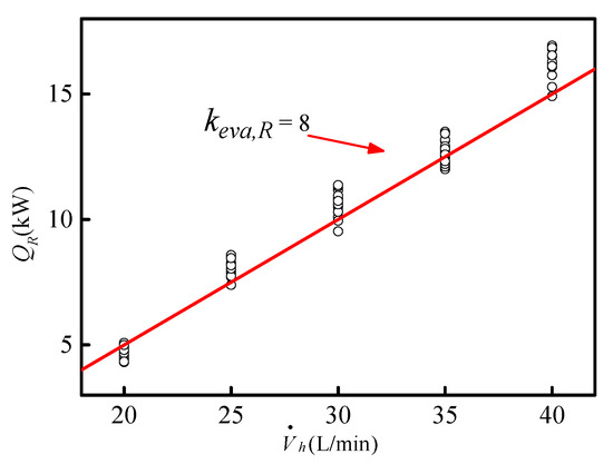
Figure 11. Heat transfer gain coefficient.

5. Conclusions

The aim of this paper was to study the helicopter electronic equipment cooling technology based on a compact plate fin ARHEx. Its experimental prototype was designed and made. More than 80 experiments were conducted to assess its heat transfer performance in certain conditions. The experimental results show the following:

(1)

The heat transfer quantity, Q_A, in the ground experiment can reach 15 kW;

(2)

The heat transfer efficiency, η₀, in the ground experiment can reach 40–80%;

(3)

The heat transfer formula of the antifreeze side can be deduced as Nu = 0.5·Re^1.396·Pr^0.4;

(4)

The heat transfer gain factor of the refrigerant side, k_eva,R, is 8, and the pressure drop gain factor of refrigerant side, k_dp, is 1.

References

- Sprouse, J. F22 Environmental Control/Thermal Management Fluid Transport Optimization. SAE Tech. Paper 2000, 109, 359–364. [Google Scholar]
- Pang, L.P.; Dang, X.M. Study on Heat Transfer Performance of Skin Heat Exchanger. Exp. Heat Transf. 2015, 28, 317–327. [Google Scholar]
- Pang, L.P.; Xu, J.; Fang, L.; Gong, M.G.; Zhang, H.; Zhang, Y. Evaluation of an Improved Air Distribution System For Aircraft Cabin. Build. Environ. 2013, 59, 145–152. [Google Scholar]
- Gao, F.; Yuan, X.G. Fuel Thermal Management System of High Performance Fighter Aircraft. J. Beijing Univ. Aeronaut. Astronaut. 2009, 35, 1353–1357. [Google Scholar]
- McAdams, W.H.; Woods, W.K.; Bryan, R.L. Vaporization inside horizontal tubes-II-Benzene-oil mixtures. Trans. ASME 1942, 64, 193. [Google Scholar]
- Emo, S.; Ervin, J.; Michalak, T.E.; Tsao, V. Cycle-based vapor cycle system control and active charge management for dynamic airborne applications. SAE Tech. Paper 2014. [Google Scholar] [CrossRef]
- Tunc, I.; Mehmet, A. Light weight high performance thermal management with advanced heat sinks and extended surfaces. IEEE Trans. Compon. Packag. Technol. 2010, 33, 161–166. [Google Scholar]
- Zhao, M.; Pang, L.; Liu, M.; Yu, S. Control strategy for helicopter thermal management system based on liquid cooling and vapor compression refrigeration. Energies 2020, 13, 2177. [Google Scholar]
- Selvaraju, A.; Mani, A. Experimental investigation on R134a vapor injector refrigeration system. Int. J. Refrig. 2006, 29, 1160–1166. [Google Scholar]
- Juan, C.; Fernando, L.; Tiejun, Z. Vapor compression refrigeration cycle for electronics cooling. Int. J. Heat Mass Transf. 2013, 66, 922–929. [Google Scholar]
- Yang, S.M.; Tao, W.Q. Heat Transfer; Higher Education Press: Beijing, China, 2006. (In Chinese) [Google Scholar]
- Genić, S.B.; Jaćimović, B.M.; Janjić, B. Experimental research of highly viscous fluid cooling in cross-flow to a tube bundle. Int. J. Heat Mass Transf. 2007, 50, 1288–1294. [Google Scholar]
- Genic, S.; Jaćimović, B.M.; Janjić, B. A computational analysis of a methanol steam reformer using phase change heat transfer. Energies 2020, 13, 4324. [Google Scholar]
- Genić, S.B.; Jaćimović, B.M.; Vladić, L.A. Heat transfer rate of direct-contact condensation on baffle trays. Int. J. Heat Mass Transf. 2008, 51, 5772–5776. [Google Scholar]
- Genić, S.; Jaćimović, B.; Jarić, M.; Budimir, N.; Dobrnjac, M. Research on the shell–side thermal performances of heat exchangers with helical tube coils. Int. J. Heat Mass Transf. 2012, 55, 4295–4300. [Google Scholar]
- Genic, S.; Jaćimović, B.M.; Vladić, L.A. Air side heat transfer coefficient in plate finned tube heat exchangers. Exp. Heat Transf. 2020, 33, 388–399. [Google Scholar]
- Genic, S.; Jaćimović, B.M.; Milovančević, U.M.; Ivošević, M.M.; Otović, M.M.; Antić, M.I. Thermal performances of a black box” heat exchanger in district heating system. Heat Mass Transf. 2018, 54, 867–873. [Google Scholar]
- Maithani, R.; Kumar, A. Correlations development for Nusselt number and friction factor in a dimpled surface heat exchanger tube. Exp. Heat Transf. 2020, 33, 101–122. [Google Scholar]
- Zhang, C.; Wang, D.; Han, Y.; Zhu, Y.; Peng, X. Experimental and numerical investigation on the exergy and entransy performance of a novel plate heat exchanger. Exp. Heat Transf. 2017, 30, 162–177. [Google Scholar]
- Gorgy, E.; Eckels, S. Convective boiling of R-134a on enhanced-tube bundles. Int. J. Refrig. 2016, 68, 145–160. [Google Scholar]
- Dossat, R.J.; Horan, T.J. Principles of Refrigeration; Prentice Hall: Upper New Jersey River, NJ, USA, 2002. [Google Scholar]
- Gnielinski, V. New equations for heat and mass transfer in turbulent pipe and channel flow. Int. Chem. Eng. 1976, 16, 359–368. [Google Scholar]
- Churchill, S.W. Friction-factor equation spans all fluid flow regimes. Chem. Eng. 1977, 84, 91–92. [Google Scholar]
- Dukler, A.E.; Wicks, M.; Cleveland, R.G. Pressure drop and hold-up in two-phase flow Part A: A comparison of existing correlations Part B: An approach through similarity analysis. AIChE J. 1964, 10, 38–51. [Google Scholar]
- Jung, K.M.; Krishnan, R.A.; Kumar, G.U.; Lee, H.J. Experimental study on two-phase pressure drop and flow boiling heat transfer in a micro pin fin channel heat sink under constant heat flux. Exp. Heat Transf. 2020, 1–24. [Google Scholar] [CrossRef]
- Junqi, D.; Yi, Z.; Gengtian, L.; Weiwu, X. Experimental Study of Wavy Fin Aluminum Plate Fin Heat Exchanger. Exp. Heat Transf. 2013, 26, 384–396. [Google Scholar]
- Shibahara, M.; Liu, Q.S.; Hata, K.; Fukuda, K. Boiling heat transfer and CHF for subcooled water flowing in a narrow channel due to power transients. Exp. Heat Transf. 2020, 33, 64–80. [Google Scholar]
- Minhhung, D.; Thanhtrung, D.; Xuanvien, N. The effects of gravity on the pressure drop and heat transfer characteristics of steam in microchannels: An Experimental Study. Energies 2020, 13, 3575. [Google Scholar]
Publisher’s Note: MDPI stays neutral with regard to jurisdictional claims in published maps and institutional affiliations. |
© 2020 by the authors. Licensee MDPI, Basel, Switzerland. This article is an open access article distributed under the terms and conditions of the Creative Commons Attribution (CC BY) license (http://creativecommons.org/licenses/by/4.0/).