Abstract
The size of wind turbine rotors is still rapidly increasing, though many technical challenges emerge. Novel rotor designs emerge to satisfy this up-scale trend, such as downwind load-aligned concepts, which orients the loads along the blade spanwise to greatly decrease the bending moments at the root. As the studies on the aerodynamics of these rotor concepts using 3D body-fitted mesh are very limited, this paper establishes different cone configurations based on the DTU 10 MW reference rotor and conducts a series of simulations. It is found that the cone angle and the distance from the blade section to the tip vortex are two deterministic factors on conning. Upwind rotors have larger power output, less thrust, smaller wake deficit, and smaller influencing area than downwind rotors of the same size, which provides superior aerodynamic priority and benefits wind farm design. The largest upwind cone angle of 14.03°, among the cases studied, leads to the highest torque to thrust ratio which is 3.63% higher than the baseline rotor. The downwind load-aligned rotor, designed to reduce the blade root bending moments at large wind speed, performs worse at the present simulation conditions than an upwind rotor of the same size.
1. Introduction
Wind energy is an important renewable energy source. On one side, the number of wind turbines has significantly increased year by year since the 1970s [1]. On the other hand, the size of wind turbines has remarkably augmented although Loth et al. [2] over-predicted the increase in 2012 and (European Wind Energy Association) EWEA under-predicted the increase in 2009. With the trends towards offshore and the requirement of a further reduction in the cost of energy (COE), single wind turbines are expected to reach a power level of 20 MW with rotor diameters in the order of 170–240 m [2]. However, the blade mass increases cubically or sub-cubically with its blade length [3]. It is estimated that the mass per blade could surpass 75,000 kg for a 20 MW three-bladed turbine [2]. As a result, the other components of a 20 MW wind turbine need to be stronger, such as the tower, transmission system, and foundation. There will be many challenges in the design and construction of such a large system. So, the cubically increasing rule of blade mass should be suppressed. Normally, the blade mass can be reduced by utilizing stronger materials, optimizing the structure of the blade, and adopting advanced controls. However, the use of stronger materials and advanced control technologies is confined by its cost [2]. Optimizing the blade structure [4,5,6] reduces the blade mass as a conventional strategy, which cannot substantially influence the cubically increasing rule.
From an optimization study of a 5 MW wind turbine rotor [6], it was found that the maximum tip displacement or rigidity of blade constrains the further reduction of blade mass, which implies the significance of larger tip-tower clearance. Measures or designs, such as coned, tilted, and pre-bending rotor concepts, lead to a larger tip-tower clearance and have been widely utilized in the wind industry. The idea of coned or tilted rotors is not new, and a brief introduction about coned rotors was given by Crawford [7]. He mentioned that a coned rotor can alleviate the static and dynamic loads, which will greatly reduce the blade weight and cost. Pre-bending blades are manufactured with its stacking line flexed toward the wind. Compared with coned and tilted rotors, pre-bending blades can be mounted on the nacelle without adjusting the nacelle design. A novel concept, ultra-light, and load-aligned rotor was proposed by Loth et al. [2,8,9,10] and showed in Figure 1. The blade geometry of this concept orients the loads along the blade span so that the structure is mainly under tension. In contrast, a conventional blade is under cantilever forces in the downstream direction. What is more, this design has no constraint of tower clearance. It was found that a net mass saving of about 50% and an overall system cost saving of about 25% can be achieved. From the aerodynamic perspective, this concept can be classified as a downwind coned rotor, which may bring a bright future for the next generation of large-scale wind turbines.
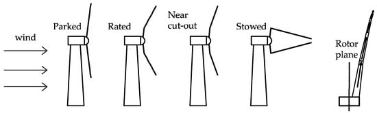
Figure 1.
Ultra-light load-aligned concept. Reproduced with permission from [9], AIAA, 2013.
Understanding the aerodynamics of these rotor concepts is the foundation of all these promising designs and concepts. However, previous research on the aerodynamics of coned, tilt, and pre-bending rotors are not abundant. Firstly, computational fluid dynamics (CFD) methods were adopted in studies. Madsen and Rasmussen [11] studied the aerodynamics of four downwind rotors with different stacking lines using an axis-symmetric actuator disc (AD) method. It has been found that the out of plane bending greatly changes the spanwise distribution of axial induction and power coefficient. A similar influence of coning on induced velocities was also observed by Mikkelsen et al. [12] using an AD CFD method. They also found that the power coefficient of upwind coning is 2–3% higher than that of downwind coning. Steele et al. [8] conducted CFD simulations for an ultra-light load-aligned (demonstrated in Figure 1) 10 MW rotor and a conventional 10 MW rotor. It is found that the spanwise distributions of the torque and thrust vary for the two rotors. Nevertheless, only one coned configuration is not enough to clearly understand the influence of coning. Winglets [13] can be treated as special conning, which cone near the blade tip. Farhan et al. [14] studied the effect of winglets through CFD simulations, which can be seen as a partially coned blade. It is observed that a winglet pointing to the downwind direction may influence the pressure distribution at 98% and 95% radial positions. Besides, the influence of the winglet may even extend to the 30% radial section at high wind speeds. In other words, the aerodynamic performance of the un-coning or un-curved part of the blade was influenced by the deformed part. This conclusion can also be obtained from the study in [11]. Bazilevs et al. [15] proposed a method to design the pre-bending shape of the blade using one-way fluid-structure interaction. However, no aerodynamic analysis was provided about the pre-bending blade.
In most design work, less time-consuming methods, such as the Blade Element Momentum (BEM) method and Vortex Method (VM), were utilized. In addition to AD CFD, Mikkelsen et al. [12] also adopted the BEM method to analyze a coned rotor with a proper decomposition of the inflow velocity. It was revealed that distinct errors may appear when the traditional BEM method is applied to rotors with large coning or blade deflections, which was also concluded by Madsen et al. [11]. Besides the proper decomposition of the inflow velocity in the rotor plan, Crawford [7,16] also corrected the velocity component in the BEM method using a vortex method. It is also shown that the radial variations of forces and velocity inductions are similar to the results from AD CFD simulations. Chattot [17] studied the effects of different wind turbine blade tip configurations, such as sweep, bending, and winglets, using the lifting line method. It is shown that partial bending influences the whole blade and an upwind bending blade can produce a larger power than that of a downwind bending blade, which is consistent with references [11,12,14]. Chattot also mentioned that further studies are needed to understand the nonlinear behaviors related to the blade bending. Shen et al. [18] optimized wind turbine blades, which have a 3D-curved stacking line with both swept in the rotor plane and bending out of the rotor plane, utilizing the lifting surface method as the aerodynamic tool. They found that the bending of the blade tip out of the plane can influence the aerodynamic of the whole blade, which is similar to the findings mentioned above.
As has been discussed above, coning or bending configurations may play an important role in the design of the next-generation super-large wind turbines. Nevertheless, the studies and references available are not enough to understand the effects of coning and bending on aerodynamics. Additionally, CFD simulations with a three-dimensional (3D) body-fitted mesh on these rotors are rare. Lastly, the winglet can be seen as a partially coned configuration and bending as a “complex” coning design. Therefore, figuring out the influence of coning is the basis of understanding winglets and bending. A rated power of 10 MW is an entry-level for the next-generation super-large wind turbines, which are expected to reach the 20 MW level and may show different aerodynamic characteristics as compared to existing commercial turbines. In conclusion, the rest of this paper will present the latest findings on the influences of coning on a 10 MW rotor and will be organized in the following three sections: descriptions of different conning configurations and CFD validations; comparisons of force distributions and other aerodynamic performances; conclusions of the present paper.
2. Modeling
2.1. Description of the Coning on the DTU 10 MW Rotor
The DTU 10 MW Reference Wind Turbine [19,20] (DTU 10MW RWT) rotor without coning and prebending is selected as the baseline in this study. The FFA-W3 airfoil series are used along with the whole blades of the DTU 10MW RWT rotor whose radius is 89.16 m. The nacelle and hub were not considered to focus on the effects of purely coning or bending. Coning will make the stacking line of the blade translate out of the rotor plane. In this paper, the displacement Zcone at a radial position r is defined by the following equation
where R is the rotor radius, Ttrans is the relative radial position where the blade starts to cone, Ccone is the cone factor controlling the slope of the stacking line. Ttrans = 5/R, 1/3, and 2/3 are utilized in this study to make the rotors start to cone at three different radial positions. It should be pointed out that Ttrans is a dimensionless number. For simplification, 5 m/89.16 m is abbreviated as 5/R. If Ccone equals ±4, ±8, ±16, and Ttrans = 5/R, six coned rotor configurations will be obtained and shown in Figure 2a. They begin to cone at the same turning point, however, with different slopes. For Ttrans = 1/3 and 2/3, the corresponding stacking lines are depicted in Figure 2b,c respectively. All of the above-coned configurations are combined in Figure 2d, where no legend is provided due to the limited space. They have the same projected areas if projected to the original straight-blade rotor plane, which is convenient for comparing the aerodynamic performances of different designs. When , the gradient of the stacking line is 1/Ccone which is independent of Ttrans. For example, the coned stacking line of Ccone = 4 and Ttrans = 5/R is parallel to that of Ccone = 4 and Ttrans = 1/3. When Ccone = ±4, ±8, ±16, the blades have cone angles of ±14.0362°, ±7.1250°, and ±3.5763°. The larger |Ccone| means the smaller cone angle, and a positive Zcone implies a coning to the downwind. Lastly, the rotors have the same distribution of airfoils, chord, and twist.
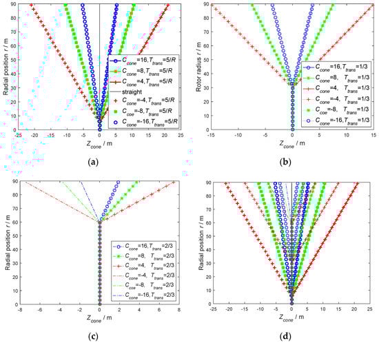
Figure 2.
Different coning configurations with ±4, ±8, ±16: (a) Ttrans = 5/R, (b) Ttrans = 1/3, (c) Ttrans = 2/3, (d) all of the configurations.
In summary, one standard rotor with in-plane straight blades and different coned configurations will be studied. Some typical rotor configurations are depicted in Figure 3. and the wind direction is from the negative Z to the positive Z.
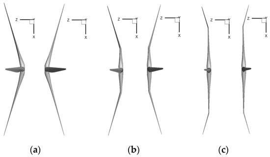
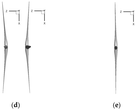
Figure 3.
Shapes of coning configurations: (a) Ccone = ±4 and Ttrans = 5/R, (b) Ccone = ±4 and Ttrans = 1/3; (c) Ccone = ±4 and Ttrans = 2/3; (d) Ccone = ±16 and Ttrans = 1/3; (e) straight.
2.2. Description of the Coning on the DTU 10 MW Rotor
The standard DTU 10MW RWT rotor with in-plane straight blades is the baseline in this study and was also simulated in other references [19,20,21]. This standard rotor is used for validating the CFD tools and other methods utilized in this paper. Three levels of grids were investigated for a grid independency study, which are named Fine gird, Middle gird, and Coarse gird. The three levels use the same standard O-O mesh configuration, whose flow field is a globe with a radius of approximately 17R as is shown in Figure 4. The first cell heights away from the blade surface are m to satisfy Y+ > 2. They all have 432 blocks, but with a different number of grid cells varying from 0.22 to 14.16 million. For Fine grid, the surface mesh on one blade contains 256 cells in the chordwise direction and 128 cells in the spanwise direction. The surface mesh expands to the far-field boundary with 128 cells along the normal direction. For Middle grid and Coarse grid, the detailed grid parameters are listed in Table 1.
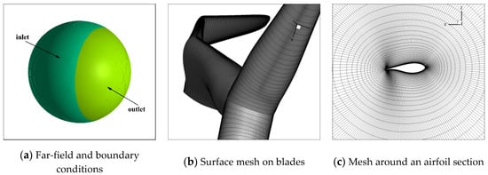
Figure 4.
Mesh and far-field boundary.

Table 1.
Grid parameters and performances of grid independency study.
For the grid independency validations, the operating condition of the DTU 10 MW RWT rotor at a wind speed of 9 m/s is selected, at which the flow is attached on most of the rotor blades and unsteady effects are negligible. The operational parameters of this standard rotor are listed in Table 2, which is also used for the cone simulations in Section 3. The CFD solver is EllipSys3D which is developed at the Technical University of Denmark [22]. The flow is treated as incompressible and fully-developed and is simulated by the steady Reynolds-Averaged Navier–Stokes (RANS) equations with the model by Menter et al. [23]. The pressure and velocity are solved with the SIMPLE algorithm. At the upstream part of the far-field boundary, shown in Figure 4a, the inlet conditions are specified with three velocity components, turbulent kinetic energy, and specific dissipation rate. The outlet conditions are specified with a fully developed flow assumption or zero normal pressure gradient [22]. The rotor surface is treated as no-slip wall conditions. The orthogonal mesh around a typical airfoil section is shown in Figure 4c. The simulation is carried out on a high-performance computer (HPC) with 144 processors utilized. For the Fine mesh configuration, the simulation cost is around 12 h. The thrust and torque of the three levels of grids are listed in Table 1. The tangential and thrust forces per unit length are compared in Figure 5. The Coarse grid cannot correctly predict the tangential force with a torque deviation of up to 74.82%. The Middle grid decreases the relative error of torque to 1.99% with 1.77 million cells, which is eight times the number of the Coarse grid. The Fine mesh uses 14.16 million cells which further reduces the relative error, with 0.91% on thrust and 0.31% on torque. Only a minor improvement can be obtained even if more cells were used and Fine grid reaches the grid convergence condition.
Table 2.
Operational parameters of the DTU 10MW RWT rotor.
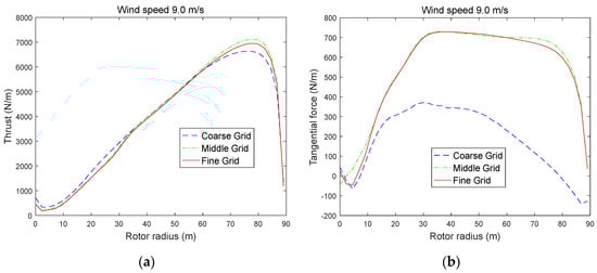
Figure 5.
Performances of grid independency study: (a) thrust force; (b) tangential force.
3. Results and Discussions
3.1. Coning the Rotors from the Same Position with Different Cone Angles
(1) Six coning with Ttrans = 5/R.
For the rotor starting to cone at r = 5 m, the spanwise distributions of rotor force and torque (sum of the values from three blades) at a wind speed of 9 m/s are depicted in Figure 6. The tangential force drives the rotor to rotate along the tangential direction and the normal force is parallel to the rotor axis. The tangential force per unit span length Ft varies along the radial position and between the different rotors. It is interesting to note that the lines of Ft intersect at the approximate position of r = 2R/3, as shown in Figure 6a. When r < 2R/3, the downwind rotor configurations, with a positive Ccone, have larger Ft than the corresponding upwind rotor configurations. The situation reverses in the outer part of the blades where larger forces appear on the upwind configurations and lower forces on the downwind cases. What is more, the downwind coning with Ccone = 4 and the upwind counterpart with Ccone = −4 have almost the reverse Ft distribution relative to the standard rotor (with in-plane straight blades). Other corresponding groups (Ccone = ±8, ±16) show the same phenomenon as well. The distribution of torque per unit span length Tt, which equals Ft multiplied by r, is shown in Figure 6b. The differences of Tt between the coned and the standard rotor are exaggerated (especially in the outer part of the blade) by a radial position r, compared to the deviations of Ft in Figure 6a. The increment of Ft near the blade tip is more beneficial to power production than that near the blade root.
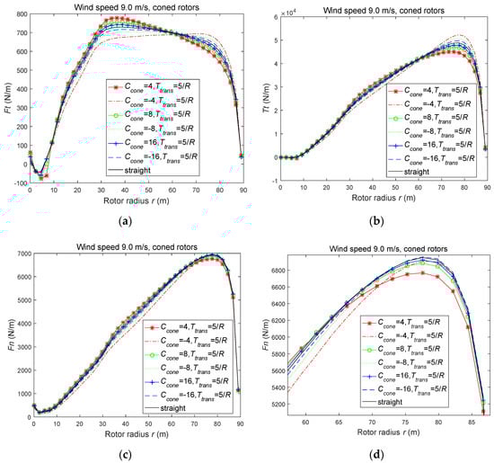
Figure 6.
Spanwise force distributions of one standard rotor and six coned configurations (Ttrans = 5/R) at 9m/s: (a) tangential force; (b) torque; (c) normal force; (d) magnified view of normal force.
The distribution of normal force per unit length Fn is shown in Figure 6c,d. The downwind rotors have larger Fn than the straight rotor when r < 2R/3, and gradually give lower Fn lines when r is further towards the blade tip. However, the Fn lines of upwind rotors gradually get close to that of the straight rotor when r > 2R/3, which is different from the enlargement phenomenon of Ft lines. Although the largest downwind cone angle (Ccone = 4) leads to the lowest Fn near the blade tip, the largest upwind cone angle (Ccone = −4) gives the overall lowest Fn. Furthermore, Ccone = −4 brings the largest Ft and Tt values near the blade tip, which is beneficial for wind turbine design.
The integrated thrust T and torque Q of these rotors are listed in Table 3. As a higher torque and a lower thrust are favorable, it comes very naturally that we use the torque to thrust ratio (torque Q divided by thrust T) to judge the overall influence of conning. This parameter is defined as QT and listed in Table 3. The relative variations of these parameters are denoted as δT, δQ, and δQT, respectively, which are also listed in Table 3. The parameter δT is defined as Equation (2), and δQ, δQT follow similar definitions.
Table 3.
Thrust and torque of one standard rotor and six coned configurations (Ttrans = 5/R) at wind speed 9 m/s.
The integrated thrust of Ccone = −4 is the lowest among these seven cases, which is 4.53% less than that of the straight rotor. Though this largest upwind conning design leads to a 1.07% reduction of torque, it still has the highest torque to thrust ratio QT due to the spectacular dwindling of thrust. In short, Ccone = −4 gives the best result. The downwind counterpart with Ccone = 4 produces the largest thrust, lowest torque, and lowest QT, which makes it the most undesirable design. The upwind configuration surpassing their downwind counterpart was also revealed in the pairs of Ccone = ±8 and ±16. The pair Ccone = ±16 (with the smallest conning slope) gives the slightest variations of T, Q, and QT. The pair Ccone = ±8 shows median variations, which is in line with our intuition.
(2) Coning at Ttrans = 1/3 and 2/3.
For the rotors with Ttrans = 1/3 and 2/3, the spanwise force distributions at a wind speed of 9 m/s are shown in Figure 7. It is interesting to see that Tt also intersects at the approximate position of r = 2R/3, which is similar to the phenomenon shown in Figure 6. It also holds true that at r < 2R/3, the downwind and upwind rotors have a larger and a smaller Tt force than the straight rotor, respectively. And at r > 2R/3, the opposite distribution appears. For Fn lines, the situation is also similar to those in Figure 6. The downwind rotors have a larger Fn at r < 2R/3, and gradually give lower Fn lines when r > 2R/3. The upwind rotors get close to the straight rotor when r > 2R/3.
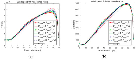
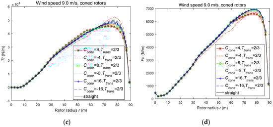
Figure 7.
Comparison of spanwise force distributions at wind speed 9m/s: (a) Ttrans = 1/3, torque force; (b) Ttrans = 1/3, normal force; (c) Ttrans = 2/3, torque force; (d) Ttrans = 2/3, normal force.
The upwind coning configurations have a lower T and a larger Q as compared with their downwind counterparts, as listed in Table 4 and Table 5, which implies the priority of the upwind design. From the view of QT, the configuration Ccone = −4 (upwind rotor with the largest cone angle) also gives the best results. It gives the largest thrust reduction with a minor loss of torque. The downwind counterpart Ccone = 4 has the worst performance with the largest thrust and the lowest torque.
Table 4.
Thrust and torque of one standard rotor and six coning configurations (Ttrans = 1/3) at wind speed 9 m/s.
Table 5.
Thrust and torque of one standard rotor and six coning configurations (Ttrans = 2/3) at wind speed 9 m/s.
The axial velocity contour in plane x = 0 m (of the coordinate system shown in Figure 3) of three rotors are shown in Figure 8. Two rotors with Ccone = ±4 and Ttrans = 1/3 are compared along with the straight rotor. It is found that the downwind rotor has the strongest wake deficit. According to the momentum theory, this will lead to the largest thrust force, which is consistent with the results shown in Table 4. The upwind rotor has the weakest deficit and the minimum thrust force. What is more, the upwind rotor has the lowest spanwise wake expansion. More wind turbines can be installed on a wind farm if upwind rotors are utilized instead of the downwind and straight rotors. So, the priority of upwind rotors lies not only in the force performance but also in the wind farm construction.
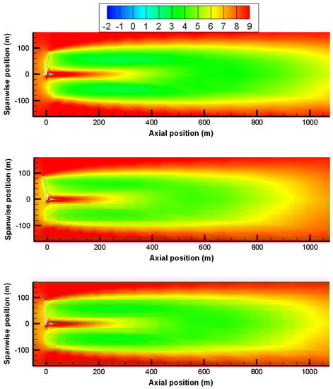
Figure 8.
Axial velocity contours on plane x = 0 m: (up) Ttrans = 1/3 and Ccone = 4; (middle) Ttrans = 1/3 and Ccone = −4; (down) straight rotor.
3.2. Coning the Rotors from Different Positions with the Same Cone Angle
From Section 3.1, it is found that the rotors with Ccone = −4 have better performanceinspite of different conning locations (Ttrans = 5/R, 1/3, 2/3). And the rotors with Ccone = 4 have worse performance. So, in this section, the rotors with the same cone angle are compared together.
(1) Rotors with Ttrans = 5/R, 1/3.
Firstly, four upwind rotors configurations with Ttrans = 5/R, 1/3 are compared, whose conning configurations are shown in Figure 9a. In the range of R/3 < r < R, the two upwind rotors have the same conning angle. In addition, as has been described in Section 2.1, the two rotors have the same chord, twist, and airfoil at the same radial location. In other words, the running condition on rotor Ccone = −4 and Ttrans = 5/R are the same as that on rotor Ccone = −4 and Ttrans = 1/3, as long as r > R/3. Based on the above knowledge, we can guess intuitively that the two upwind rotors will perform similarly in the range R/3 < r < R. And the simulation results, as shown in Figure 9b–d, have revealed our initial guess. In the range of R/3 < r < R, the respective Ft and Fn distributions of the two upwind rotors are very close.
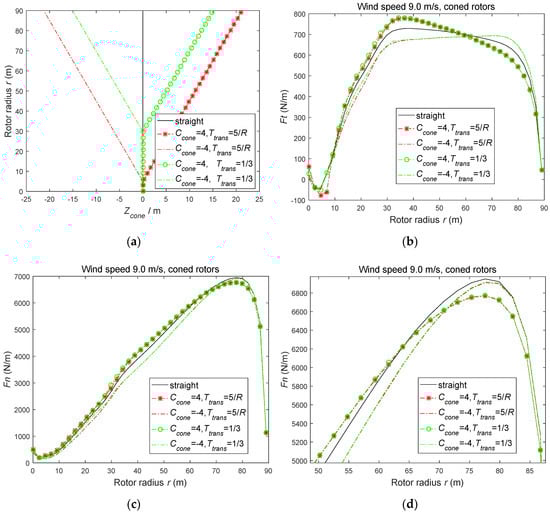
Figure 9.
Comparisons of rotors with Ttrans = 5/R, 1/3: (a) conning configurations; (b) tangential force; (c) normal force; (d) magnified view of normal force.
In the range of 5 m < r < R/3, the discrepancy between lines in Figure 9b,c are obvious. This discrepancy is caused by the different conning configurations where Ttrans = 5/R has a cone angle and Ttrans = 1/3 is without cone. This phenomenon indicates that the conning slope is a fundamental parameter when considering the effects of the cone. The two downwind rotors also show a similar phenomenon. Although rotor with Ttrans = 1/3 has zero Zcone in this range, it does not produce the same force distributions as the straight one. This implies that different cone configurations at r > R/3 influence the blade sections at 5 m < r < R/3, even if they all have zero cone angle there.
(2) Rotors with Ttrans = 1/3, 2/3.
Secondly, the up/downwind counterparts of Ttrans = 1/3 are compared with counterparts of Ttrans = 2/3. The conning configurations are shown in Figure 10a. In the range of 2R/3 < r < R, the two upwind rotors have the same cone angle. The two downwind rotors cone with the same slope as well. As is shown in Figure 10b–d, the Ft and Fn lines of the two upwind rotors almost coincide and as well as the downwind rotors. This phenomenon agrees well with Section 3.2(1).
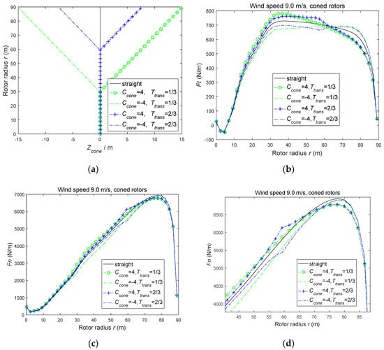
Figure 10.
Comparisons of rotors with Ttrans = 1/3, 2/3: (a) conning configurations; (b) tangential force; (c) normal force; (d) magnified view of normal force.
In the range of R/3 < r < 2R/3, the two upwind rotors have different cone configuration so that the Ft and Fn lines do no coincide. The same holds true for the downwind rotors. Although Ttrans = 2/3 coincides with the straight configuration as is shown in Figure 10a, they produce different force distributions. In the range of r < R/3, all the rotors are not conning. However, their force distributions deviate from each other. Similar to Section 3.2(1), conning on the blade tip will influence the spanwise region extending to the blade root. However, the different cone designs on the spanwise region away from the blade tip (such as R/3 < r < 2R/3) do not influence the blade tip region (r > 2R/3). Cone on regions with larger r has priority over smaller r, which shows the importance of blade tip design.
3.3. Coning the Rotors from Different Positions with the Same Blade Tip Position
It has been found in Section 3.2 that the different cone designs on the middle span region (such as R/3 < r < 2R/3) do not influence the blade tip region (r > 2R/3). However, the cone on the blade tip region could influence the rest of the blade. This implies the importance of the blade tip. In this section, rotors with the same tip locations are selected for comparison.
As is shown in Figure 11, the rotor of Ccone = 8, Ttrans = 1/3 and the rotor of Ccone = 4, Ttrans = 2/3 have the same tip displacement Zcone = R/12. For Ccone = −8, −4, the tip displacement is Zcone = −R/12. In the range of r < R/3, all the rotors have zero Zcone. It is interesting that the Ft and Fn lines of the two upwind rotors almost coincide at r < R/3, which never appears in figures of Section 3.1 and Section 3.2. The downwind rotors also show the same rule. It is validated that, when considering the effects of conning on the non-cone part, the blade tip position is a critical parameter. If the partially coned configurations have the same tip position, the part without cone will perform the same.
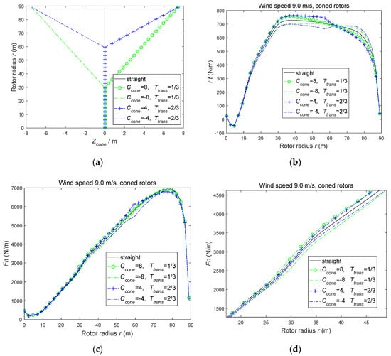
Figure 11.
Comparisons of rotors with the same tip location: (a) conning configurations; (b) tangential force; (c) normal force; (d) magnified view of the normal force.
The pressure coefficient Cp at different blade sections is depicted in Figure 12, whose horizontal axis is normalized by the local chord length. At r = 15.97 m and 50.20 m, upwind coned configurations have smaller integration areas closed by the Cp curves. At r = 79.87 m, downwind rotors have a notably smaller integration area. These are consistent with the smaller Fn of upwind rotors in Figure 11. At r = 61.61 m, the two rotors with Ttrans = 1/3 have similar Cp curves as the straight rotor. Among the two rotors with Ttrans = 2/3, the upwind one has a smaller Cp integration area, and the downwind has a larger area. They are all compatible with the Fn lines. However, from Figure 12c, it is hard to find why the Ft lines of the two rotors with Ttrans = 2/3 intersect in Figure 11b.
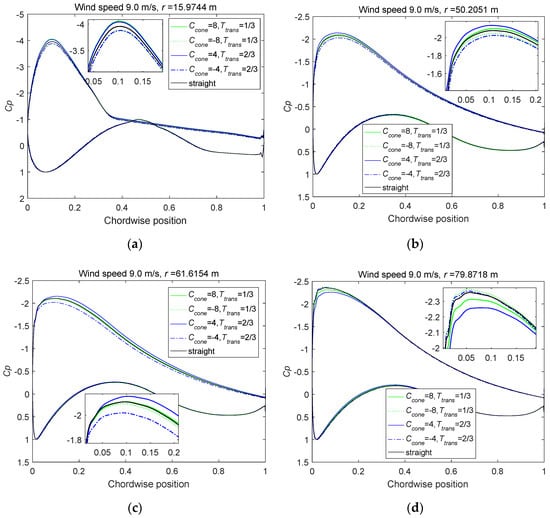
Figure 12.
The pressure coefficient distributions at four radial positions (horizontal axis is normalized by the local chord length): (a) r = 15.9744 m, (b) r = 50.2051 m, (c) r = 61.6154 m, (d) r = 79.8718 m.
To find the relationship with Ft, the Cp curves are not drawn along the chordwise direction. Instead, as shown in Figure 13, they are depicted along the rotor axial direction so that the integration area closed by Cp curves can reflect the Ft changes. The horizontal axis is normalized by the maximum thickness of the respected airfoil section. In Figure 13c, the special Cp distributions in the axial position range (0.5, 1), which represent the suction side, leads to an equalized Ft of the two rotors with Ttrans = 1/3. If the Cp lines in this range are observed in the clockwise direction (an axial position from 0.5 to 1, then from 1 to 0.5), the observed positions are moving from the leading edge (LE) to the maximum thickness point (MTP) and then to the trailing edge (TE). From LE to the MTP, the upwind rotor with Ttrans = 1/3 has a lower Cp than the straight rotor. From MTP to TE, the upwind one also has lower Cp. The integration areas closed by the Cp curves of the two rotors with Ttrans = 1/3 are nearly equal. In Figure 13a,b,d, the integration areas closed by Cp curves are different which leads to different Ft. Downwind coned configurations have larger integration area at r = 15.97, 50.20 m and smaller integration area at r = 79.87 m, which is consistent with the Ft lines in Figure 11b.
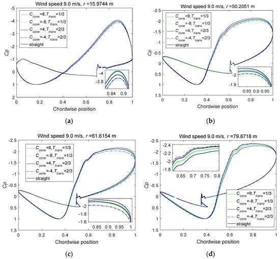
Figure 13.
The pressure coefficient distributions at four radial positions (horizontal axis is normalized by the maximum thickness): (a) r = 15.9744 m, (b) r = 50.2051 m, (c) r = 61.6154 m, (d) r = 79.8718 m.
As discussed above, the secrets of equal Ft lies in the Cp distributions on the suction side. The lines from MTP to TE in Figure 13c are different from those in Figure 13a,b,d. Back to the normally used Cp curve style in Figure 12, the suction side lines of Figure 12c are obviously different from Figure 12a,b,d. In Figure 12c, the Cp difference between up/downwind counterparts appears on the whole suction side. In Figure 12a,b,d, the Cp difference mainly show near the leading-edge suction peaks. In short, the Fn and Ft force distributions can be explained by the corresponding Cp distributions.
As is shown in Figure 12d, the Cp suction peaks of the two upwind rotors are only slightly higher than that of the straight rotor which explains the nearly coincide Fn forces near the tip. In Section 3.1 and Section 3.2, all the Fn lines of upwind rotors gradually coincide with that of a straight rotor near the tip. The reason why the Fn lines of upwind rotors do not obviously surpass that of the straight rotor at r > 2R/3 needs to be further studied. Coincidently, Prandtl’s tip loss factor F starts to be none zero at about 2R/3 which is shown in Figure 14. It is preliminarily supposed that the Fn force near the blade tip is strongly controlled by the tip loss effects, which is caused by the radial flow across the blade tip from the pressure to the suction side. Fn is directly connected with pressure on both sides. Thrust decreases dramatically near the blade tip because of tip loss effects. Therefore, it is rather hard to produce higher thrust near the blade tip regardless of upwind or downwind configurations. Furthermore, the upwind cone will decrease the spanwise tip loss velocity because of the projection of axial velocity and then decrease the tip loss effects. This is consistent with the slightly higher suction peak of upwind rotors in Figure 12d. Downwind cone will increase the spanwise velocity and the tip loss, which agrees with the lower suction peaks in Figure 12d and lower thrust in Figure 11c.
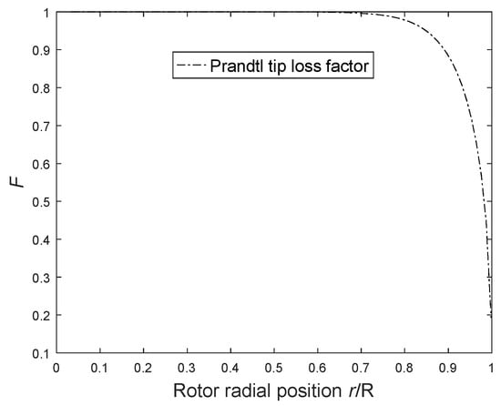
Figure 14.
The distribution of Prandtl tip loss factor F.
The vorticity contour on plane x = 0 m of different rotors are compared in Figure 15. At approximately r > 2R/3, the blade sections are surrounded by tip vortex so that the tip loss effect is of vital importance. Consistent with the analysis above, downwind rotors have stronger tip vorticity than the upwind counterparts. Therefore, downwind rotors have larger power loss and lower Fn force in this range. At approximately r < 2R/3, the tip loss effect is weak. However, the shed vortex still influences the blade force through induction. According to the Biot–Savart law, the wind speed induction decrease with the square of distance away from the vortex center. So, the distance from the blade section to the tip vortex is of vital importance. And the distances vary with the cone configurations. The downwind rotors push the tip vortex further downstream, which leads to less tip vortex induction and higher axial inflow velocity. As a result, the Fn force of downwind rotors are larger than the upwind counterparts and the straight rotor in this range, which is consistent with the thrust distributions in Section 3. In short, the different cone configuration leads to different cone angle, different tip vortex strength and different position of tip vortex, which then determines the final force distributions along the rotor span.
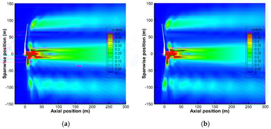
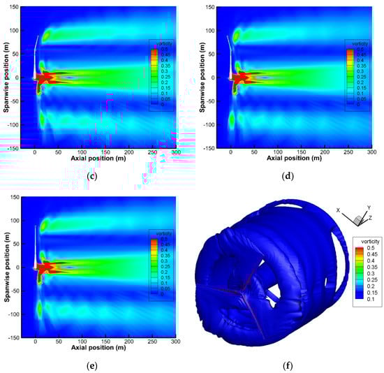
Figure 15.
The vorticity contour on plane x = 0 m: (a) rotor of Ttrans = 1/3 and Ccone = 8; (b) rotor of Ttrans = 1/3 and Ccone = −8; (c) rotor of Ttrans = 2/3 and Ccone = 4; (d) rotor of Ttrans = 2/3 and Ccone = −4; (e) straight rotor; (f) vorticity isosurface of straight rotor.
4. Conclusions
Special coning, bending, or winglet configurations may play an important role in the design of the next-generation super-large wind turbines. Figuring out the influence of coning is the basis of understanding winglets and bending. However, CFD simulations on all kinds of coned rotors with 3D body-fitted mesh are rare. Therefore, this paper presents the latest findings on the influences of coning with a 10 MW reference rotor. Although only the force, pressure coefficient distributions and some flow field contours are compared, the available results may be useful for designing coned rotors and shed light on bending and winglet designs.
Firstly, the upwind conning blade can produce larger power than that of the downwind counterpart, which is consistent with references in Section 1. At least among cases with Ccone = ±4, ±8, ±16 (cone angles of ±14.0362°, ±7.1250°, ±3.5763°), the largest upwind cone Ccone = −4 leads to the lowest thrust force with few reductions of torque. If torque to thrust ratio is used to judge the performance of conning, Ccone = −4 leads to 2–3% higher performance according to the exact cone starting position.
Secondly, the cone angle and blade tip position are two important factors to determine the influences of the cone. If coned configurations have the same cone angle, the coned sections will suffer the same force distribution. If coned configurations have the same blade tip position, the un-coned sections will have the same performance. The radial position r = 2R/3 is an interesting turning point across which the up/downwind counterparts have nearly reverse tangential force distribution relative to the straight rotor. The thrust show less symmetric distributions near the blade tip due to the strong tip loss effects.
The priority of upwind conning rotors lies not only in aerodynamics but also in wind farm layout. Upwind conned rotors have a weaker deficit, smaller wake influencing area, therefore more wind turbines can be placed in a given wind farm area. From aerodynamics and wind farm aspects, the downwind ultra-light load aligned rotor mentioned in Section 1 was not superior to upwind coned configurations. However, the ultra-light load aligned rotor has great advantages under extreme large wind condition over traditional rotors, which has been thoroughly discussed and compared in Section 1. So, it is hard to say which type is of obvious priority. More studies are needed to analyze these rotors in more realistic conditions, for example, from the aeroelastic aspects under unsteady inflow. The basic analysis in the present paper can provide references for relevant rotors designs and studies.
Author Contributions
Conceptualization, Z.S. and W.J.Z.; methodology, Z.S. and W.J.Z; software, W.Z.S. and W.J.Z.; validation, Z.S., W.J.Z., and W.Z.S.; formal analysis, Z.S., W.J.Z., W.Z.S., and W.Z.; investigation, Z.S.; resources, W.J.Z. and W.Z.S.; data curation, Z.S., J.C., Q.T., and W.Z.; writing—original draft preparation, Z.S., W.J.Z., and W.Z.S.; writing—review and editing, Z.S., W.J.Z., and W.Z.S.; visualization, Z.S.; supervision, W.J.Z. and W.Z.S.; project administration, W.J.Z.; funding acquisition, Z.S. and W.J.Z. All authors have read and agreed to the published version of the manuscript.
Funding
This research was funded by the National key research and development program of China under grant number 2019YFE0192600; the National Nature Science Foundation of China under grant number 51905469 and 11672261; an open funding from Shanxi Key Laboratory of Industrial Automation under grant number SLGPT2019KF01-13.
Conflicts of Interest
The authors declare no conflict of interest.
References
- Höyland, J. Challenges for Large Wind Turbine Blades. Ph.D. Thesis, Norwegian University of Science and Technology, Trondheim, Norway, 2010. [Google Scholar]
- Loth, E.; Steele, A.; Ichter, B.; Selig, M.; Moriarty, P. Segmented ultralight pre-aligned rotor for extreme-scale wind turbines. In Proceedings of the 50th AIAA Aerospace Sciences Meeting Including the New Horizons Forum and Aerospace Exposition, Nashville, TN, USA, 9–12 January 2012. [Google Scholar]
- Fingersh, L.J.; Hand, M.M.; Laxson, A.S. Wind Turbine Design Cost and Scaling Model; National Renewable Energy Lab. (NREL): Golden, CO, USA, 2006. [Google Scholar]
- Barnes, R.H.; Morozov, E.V. Structural optimisation of composite wind turbine blade structures with variations of internal geometry configuration. Compos. Struct. 2016, 152, 158–167. [Google Scholar] [CrossRef]
- Chen, J.; Wang, Q.; Shen, W.Z.; Pang, X.; Li, S.; Guo, X. Structural optimization study of composite wind turbine blade. Mater. Des. 2013, 46, 247–255. [Google Scholar] [CrossRef]
- Sun, Z.; Sessarego, M.; Chen, J.; Shen, W.Z. Design of the OffWindChina 5-MW Wind Turbine Rotor. Energies 2017, 10, 777. [Google Scholar] [CrossRef]
- Crawford, C.; Platts, J. Updating and optimization of a coning rotor concept. In Proceedings of the 44th AIAA Aerospace Sciences Meeting and Exhibit, Reno, NV, USA, 9–12 January 2006. [Google Scholar]
- Steele, A.; Ichter, B.; Qin, C.; Loth, E.; Selig, M.; Moriarty, P. Aerodynamics of an Ultra light Load-Aligned Rotor for Extreme-Scale Wind Turbines. In Proceedings of the 51st AIAA Aerospace Sciences Meeting Including the New Horizons Forum and Aerospace Exposition, Grapevine, TX, USA, 7–10 January 2013. [Google Scholar]
- Noyes, C.; Qin, C.; Loth, E. Analytic analysis of load alignment for coning extreme-scale rotors. Wind Energy 2020, 23, 357–369. [Google Scholar] [CrossRef]
- Noyes, C.; Qin, C.; Loth, E.; Martin, D.; Johnson, K.; Ananda, G.; Selig, M. Extreme-scale load-aligning rotor: To hinge or not to hinge? Appl. Energy 2020, 257, 1–11. [Google Scholar] [CrossRef]
- Madsen, H.A.; Rasmussen, F. The influence on energy conversion and induction from large blade deflections. In Proceedings of the 1999 European Wind Energy Conference and Exhibition, Nice, France, 1–5 March 1999. [Google Scholar]
- Mikkelsen, R.; Sørensen, J.N.; Shen, W.Z. Modelling and analysis of the flow field around a coned rotor. Wind Energy 2001, 4, 121–135. [Google Scholar] [CrossRef]
- Sy, M.S.; Abuan, B.E.; Danao, L.A.M. Aerodynamic Investigation of a Horizontal Axis Wind Turbine with Split Winglet Using Computational Fluid Dynamics. Energies 2020, 13, 4983. [Google Scholar] [CrossRef]
- Farhan, A.; Hassanpour, A.; Burns, A.; Motlagh, Y.G. Numerical study of effect of winglet planform and airfoil on a horizontal axis wind turbine performance. Renew. Energy 2018, 131, 1255–1273. [Google Scholar] [CrossRef]
- Bazilevs, Y.; Hsu, M.C.; Kiendl, J.; Benson, D. A computational procedure for prebending of wind turbine blades. Int. J. Numer. Methods Eng. 2012, 89, 323–336. [Google Scholar] [CrossRef]
- Crawford, C. Re-examining the precepts of the blade element momentum theory for coning rotors. Wind Energy 2006, 9, 457–478. [Google Scholar] [CrossRef]
- Chattot, J.J. Effects of blade tip modifications on wind turbine performance using vortex model. Comput. Fluids 2009, 38, 1405–1410. [Google Scholar] [CrossRef]
- Shen, X.; Chen, J.G.; Zhu, X.C.; Liu, P.Y.; Du, Z.H. Multi-objective optimization of wind turbine blades using lifting surface method. Energy 2015, 90, 1111–1121. [Google Scholar] [CrossRef]
- Zahle, F.; Bak, C.; Sørensen, N.N.; Guntur, S.; Troldborg, N. Comprehensive Aerodynamic Analysis of a 10 MW Wind Turbine Rotor Using 3D CFD. In Proceedings of the 32nd ASME Wind Energy Symposium, National Harbor, ML, USA, 13–17 January 2014. [Google Scholar]
- The DTU 10MW Reference Wind Turbine Project Site. Available online: https://rwt.windenergy.dtu.dk/dtu10mw/dtu-10mw-rwt (accessed on 6 November 2018).
- Jost, E.; Lutz, T.; Krämer, E. Steady and unsteady CFD power curve simulations of generic 10 MW turbines. In Proceedings of the 11th EAWE PhD Seminar on Wind Energy in Europe, Stuttgart, Germany, 23–25 September 2015. [Google Scholar]
- Sørensen, N.N. General Purpose Flow Solver Applied to Flow over Hills. Ph.D. Thesis, Technical University of Denmark, Lyngby, Denmark, 1995. [Google Scholar]
- Menter, F.R. Two-equation eddy-viscosity turbulence models for engineering applications. AIAA J. 2012, 32, 1598–1605. [Google Scholar] [CrossRef]


Publisher’s Note: MDPI stays neutral with regard to jurisdictional claims in published maps and institutional affiliations. |
© 2020 by the authors. Licensee MDPI, Basel, Switzerland. This article is an open access article distributed under the terms and conditions of the Creative Commons Attribution (CC BY) license (http://creativecommons.org/licenses/by/4.0/).