Abstract
The main objective of this research was to test the effect of oil prices, renewable and non-renewable energy consumption, and economic growth on Turkey’s carbon emissions by using three co-integration tests, namely, the newly-developed bootstrap autoregressive distributed lag (ARDL) testing technique as proposed by (McNown et al., 2018); the new approach involving the Bayer–Hanck (2013) combined co-integration test; and the H-J (2008) co-integration technique, which induces two dates of structural breaks. The autoregressive distributed lag model (ARDL), dynamic ordinary least squares (DOLS), canonical cointegrating regression (CCR), and fully modified ordinary least square (FMOLS) approaches were utilized to test the long-run interaction between the examined variables. The Granger causality (GC) analysis was utilized to investigate the direction of causality among the variables. The long-run coefficients of ARDL, DOLS, CCR, and FMOLS showed that the oil prices had a negative influence on CO2 emissions in Turkey in the long run. Furthermore, the findings demonstrate that non-renewable energy, which includes oil, natural gas, and coal, increased CO2 emissions. In contrast, renewable energy can decrease the environmental pollution. These empirical findings can be attributed to the fact that Turkey is heavily dependent on imported oil; more than 50% of the energy requirement has been supplied by imports. Hence, oil price fluctuations have severe effects on the economic performance in Turkey, which in turn affects energy consumption and the level of carbon emissions. The study suggests that the rate of imported oil in Turkey must be decreased by finding more renewable energy sources for the energy supply formula to avoid any undesirable effects of oil price fluctuations on the CO2 emissions, and also to achieve sustainable development.
1. Introduction
In recent decades, Turkey’s integration into the world markets has increased as a result of the globalization of the world economy [1]. The Turkish markets are easily affected by global external shocks such as oil prices. In this regard, the main objective of this research was to provide new empirical evidence by testing the effect of oil prices on carbon emissions in Turkey using the newly-developed bootstrap autoregressive distributed lag (ARDL) technique as proposed by [2]. Furthermore, Granger causality (GC) analysis was utilized to investigate the direction of causality among the variables.
Turkey has faced several challenges in energy security, the first of which is the energy supply problem. Turkey’s main energy suppliers are Russia and Iran. It is likely that any economic or political disagreements with these countries will put energy security in Turkey at risk [3]. In this regard, Turkey should attempt to diversify its oil sources in order to reduce the dependency on the main suppliers. The second main challenge is the high dependency on imported oil. Domestic oil production in Turkey is not sufficient to meet the country’s energy needs. Despite the limitations of oil production, the demand for oil is rapidly increasing. Consequently, Turkey should evaluate alternative renewable energy sources such as solar, wind, and geothermal. These resources can be simply produced and renewed. Additionally, they emit fewer pollutants into the environment, and can never be depleted. Renewable energy resources in Turkey include hydroelectric, wind, solar, geothermal, biomass, and waves [4]. Turkey is ranked third in the world in terms of the production of geothermal energy with 1.28 million tons of oil equivalent (MTOE), and the Aegean territory, in particular, has huge geothermal energy potential. Despite the advantages of using renewable energy resources including the reduced pollutants and the fact that they cannot be depleted, the consumption of non-renewables in Turkey has consistently been elevated in line with the increase in its population. In this regard, the gas consumption in Turkey has increased from 1000 million cubic feet in 1980 to 1,720,759 million cubic feet in 2014. The coal consumption in Turkey has increased from 20,530,547 tons in 1980 to 106,463,304 tons in 2014. Furthermore, Figure 1 shows that the oil consumption in Turkey has increased from 313,200 barrels per day (B/d) in 1980 to 762,532 barrels per day (B/d) in 2014. On the other hand, the figure also shows that oil production in Turkey increased from 41,000 barrels per day in 2014 to 57,367 barrels per day in 2014. This figure confirms that domestic oil production in Turkey is not enough to meet the country’s energy needs.
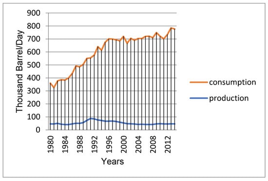
Figure 1.
Oil consumption and production over the period 1980–2014 in Turkey. Source: Author’s own calculations.
Although the 2023 vision aims to increase the use of renewable-energy sources to 30%, Turkey plans to construct 85 new “coal-fired power” stations over the period from 2020 to 2030, which could increase carbon emissions by 50% over this period [5]. In this regard, it is highly important for Turkey to adopt policies to reduce emissions, and to also invest in energy transmission and distribution channels to improve the country’s energy efficiency [6].
However, the economy of this country is one of the leading producers among the emerging countries in terms of textiles, ships, motor vehicles, consumer electronics, home appliances, construction materials, and other transportation equipment, which has led to increasing non-renewable energy consumption, particularly oil consumption. According to the literature, variations in oil prices have a powerful influence on various economic variables. In this regard, [7,8,9] have indicated that the effect of oil prices on economic indexes in developed and developing economies can be different; these different findings can be attributed to various economic factors such as oil-importing countries vs. oil-exporting countries. In this regard, increases in oil prices can be economically bad for oil-importing countries, but are economically good news for oil-exporting countries. However, Turkey is a country that imports a large proportion of its oil needs from abroad. Hence, an increase in oil prices negatively affects Turkey’s current account balance and economic growth and other economic variables [10]. In this regard, if crude oil prices increase, then inflation in oil-importing countries like Turkey will also rise, which leads to an increase in interest rates. Thus, any increase in interest rate can affect the cost of finance, which in turn leads to a reduction in investments and energy consumption. In this sense, the main objective of this research is to provide new empirical evidence by testing the impact of oil prices on Turkey’s carbon emissions through energy consumption and economic growth factors.
2. Literature Review
According to the literature, variations in oil prices have a powerful influence on various economic variables [7,8,9,10,11]. Ref. [7], the authors showed that oil prices have a significant impact on GDP in 12 European countries. [8] tested the impact of oil prices on the economic activities in Thailand. The results indicated that oil prices had a significant influence on macroeconomic variables such as investment, over the period from 1993 to 2006. Ref. [9], they tested the influence of oil prices on Turkey’s GDP over the period from 1996–2017. The results showed that any change in oil prices has a powerful impact on Turkey’s GDP. Ref. [10], the study indicated that oil prices had a powerful effect on the exchange rates in Saudi Arabia.
Some empirical papers have tested the effect of oil prices on energy consumption and the level of carbon dioxide emissions. In this regard, [11] suggested that there was a causality interaction from oil price to energy consumption in Tunisia, while [12] found that the oil price had a significant influence on energy consumption in China. [13] tested the causal linkage between oil price and the level of carbon emissions using the ARDL model. The findings indicated that there is a positive interaction between oil prices and the level of carbon emissions in Venezuela. [14] used a panel data model and demonstrated that there was a positive and statistically significant link between oil price and carbon emissions per capita in 11 South American countries from 1980 to 2010. [15] used the ARDL model, and found that the oil price had a powerful impact on emissions in Saudi Arabia. Ref. [16] tested the interaction between the level of carbon emissions and oil prices in Brazil, Russia, India, China, and Turkey using the Vector Autoregression testing model. The findings demonstrated that there is a powerful influence of oil prices on carbon emissions in Brazil, Russia, India, China, and Turkey. Ref. [17], they suggested that that an increase in international oil prices could advance the outputs and investment in renewable energies, which in turn would lead to an increase in renewable energy consumption.
Ref. [18], they utilized the ARDL testing model to investigate the effects of oil price on the level of carbon emissions in Pakistan. The findings revealed that the oil price boosted the level of carbon emissions in the short run, while decreasing the level of carbon emissions in the long-run. Ref. [19], they used the ARDL approach, and scrutinized the effects of oil prices on carbon dioxide emissions in Turkey. The findings demonstrated that there was an inverse interaction between oil prices and the levels of carbon emissions. In contrast, [20] applied the ARDL testing model, and suggested that there were no significant interactions between the oil price and carbon emissions in China.
On the other hand, several studies have demonstrated significant relationships between the use of renewable energy sources, an increase in GDP, and the reduction of emissions. As a preliminary example in this vein, Tien [21] tested the causality linkage between energy use and carbon emissions in Russia for the period of 1990 to 2007 by using the Granger causality approach. The results indicated that there is bidirectional causality between energy use and emissions in Russia. Ref. [22], they tested the influence of renewable energy and GDP on emissions in Turkey by applying the ARDL test. The findings showed that the relationship between renewable energy and GDP was significant and negatively affected emissions. In another study that also addressed Turkey, [23] tested the linkage between GDP, carbon emissions, and energy consumption in Turkey and the Caucasus for the period from 1992 to 2013 by using the VAR technique. The results suggested that renewable energy consumption had a negative and statistically significant effect on carbon emissions in Turkey. Similarly, [24] tested the effect of non-renewable energy and GDP on emissions in Italy during the period of 1960 to 2011 by employing the ARDL test. The results indicated that renewable energy and GDP were significant and negatively affected carbon emissions.
In contrast, the results of another study indicated that non-renewable energy consumption was significant and positively affected the level of carbon emissions. Ref. [25], the authors analyzed the influence of renewable energy and real income on carbon emissions in 17 selected countries for the period from 1980 to 2011 by using Panel FMOLS and DOLS tests. The results showed that the hypothesis of EKC was valid in OECD countries, and non-renewable energy consumption had a positive influence on carbon emissions in in the OECD countries. Ref. [26] also researched the OECD countries employing an AMG estimator, and found an inverse association among renewable energy consumption and the level of carbon emissions as well as a positive relation between non-renewable energy and the level of carbon emissions in the OECD countries. In another study focused on OECD countries. Ref. [27] examined the impact of renewable energy on carbon emissions in 26 OECD countries and Brazil, Russia, India, and China by using Panel FMOLS and DOLS for the period from 1980 to 2011. The results supported the positive linkage between non-renewable energy and the carbon emissions, and also revealed a negative relationship between real income, renewable energy, and emissions. [28] tested the influence of energy consumption and real income on U.S. carbon emissions from 1960 to 2010 by employing the ARDL model. The results showed that non-renewable energy consumption and GDP were significant and positively affected emissions, while renewable energy consumption had a negative effect on emissions. Ref. [1] found that nonrenewable energy consumption positively affected Turkey’s carbon emissions in the period from 1980 to 2014. However, according to the literature, there are many environmental and economic benefits of using renewable energy. For instance, [29,30] showed that the use of renewable energy would reduce the dependence on imported fuels. Ref. [31,32], they showed that that the use of renewable energy would lead to the generation of energy that produced no CO2 emissions.
3. Model and Data
In the conventional EKC model, GDP and GDP² are the major determinants of the level of carbon emissions. The reason why the conventionally squared GDP is used is that countries might have inverted U-shaped EKCs. Non-renewable and renewable energy consumption are two other major determinants of emissions. Thus, the EKC model is formulated as:
where denotes the carbon emissions; GDP and GDP² represent the economic growth and the square of GDP, respectively; NREC is the non-renewable energy consumption; and REC is the renewable energy consumption. The assumption is that environmental degradation is proxied by () emissions (kt) and regressed on (OP), (REC) (NREC), (GDP), and (GDP²). Thus, the following equation can be checked:
where represents the logarithm of the carbon emissions in kilotons is the economic growth in constant 2010 US dollars, the quadratic economic growth in constant 2010 US dollars; is Brent crude oil prices, which is generally utilized in Turkey [3]; is the logarithm of (renewable energy consumption, which is a share of total final energy consumption; is a logarithm of (non-renewable energy consumption that includes oil, natural gas, and coal in British Thermal Unit (BTU). The data in this study were collected from the BUS Energy Information Administration and World Development Indicators. The data retrieved were yearly data and ranged from 1985 to 2015.
Unit Root Tests and Cointegration Tests
To identify the cointegration among the variables, the article examined whether the data were stationary or not. The article applied unit root tests including structural breaks dates (BD) such as the Zivot–Andrews (2002) [33] and Perron–Vogelsang (1993) [34] tests with one (BD). To verify the existence of the long-run interaction between oil price, REC, and NREC, GDP, the square of (GDP), and emissions, the study applied the ARDL bounds testing approach. According to McNown et al. (2018), the autoregressive distributed lag (ARDL) bounds test as proposed by Pesaran et al. (2001) may draw incorrect findings on the status of the cointegration test if the ARDL bounds test is not implemented correctly. The newly-developed ARDL test is preferred over the traditional Pesaran (2001) cointegration tests because of its competency in predicting while addressing the issues of power and size weakness and its respective characteristics, which traditional cointegration tests fail to address. Furthermore, the bootstrap-ARDL is more suitable because it has no sensitivity with respect to the features of the integration order, while addressing the concerns of inconclusiveness of the observations, which are usually encountered during the application of the traditional ARDL cointegration tests. Hence, this study aimed to provide fresh empirical evidence by testing the effect of the oil prices, renewable and non-renewable energy consumption, and economic growth on Turkey’s carbon emissions using the new bootstrap ARDL test.
This approach was recently upgraded by McNown et al. [2], and the recent version includes the additional t-test or F-test on the estimated coefficients of the lagged independent variables. The of test is: σ1 = 0. The of the test is: ≠ 0, while the of the test is = = = = = 0. The of the test is:: ≠ ≠ ≠ ≠ ≠ 0.
The critical values (CV) in the bootstrap ARDL approach are created based on the specific integration features of each time series data using the ARDL bootstrap procedures, which in turn leads to the elimination of the unstable findings of the ARDL bounds of co-integration approach [2]. However, McNown et al. (2018) upgraded the bootstrap ARDL test by employing a table of CV gained by bootstrap simulation. These steps of the bootstrap test will lead to the acquisition of better results than the traditional ARDL bounds test (Pata, 2019) [35]. In particular, the Pesaran et al. (2001) [36] CV allows for (1) variables to be endogenous, while the CV generated with a bootstrap technique allows for the endogeneity of all explanatory examined variables. Additionally, this approach is more suitable for data that include more than (1) explanatory variable.
Moreover, the ARDL aims to estimate the short-run and long-run parameters of the model. ARDL examines the null hypothesis of no cointegration against the alternative hypothesis that cointegration exists, based on F-statistics, by comparing the Pesaran et al. (2001) critical values. If the F-statistic exceeds the upper bound I(1), the will be rejected, thus the co-integration between the data series is valid. However, if the F-statistic values are less than the lower bound I(0), the (no cointegration) will be accepted. Moreover, if the F-statistic values are between I(0)–I(1), the inference would be inconclusive.
The testing of the ARDL model is as follows:, , , , is formulated in the next equation:
where ∆ means the first difference operator, and , , , and variables are the logarithms of the tested variables; K represents the optimal of lags; and denotes the error-disturbance of the model. The error correction model is presented by the next equation to determine the speed of adjustment:
where Δ represents a change in , ,, and variables. However, Error Correction Tern () is expected to be statistically significant with a negative sign; this sign implies the velocity of adjustment in the short- and long-run levels.
Furthermore, the Bayer and Hanck (2013) [37] technique was applied to confirm the results of the ARDL testing model. The main advantage of this test is that it can be utilized for time series with a different order of integration and combines four different cointegration approaches, namely, (1) Engle and Granger (1987) [38], (2) Johansen (1988) [39], (3) Boswijk (1994) [40]; and Banerjee et al. (1998) [41]. However, this test includes the Fisher F-statistics to provide powerful evidence to confirm the cointegration. Based on Fisher’s formula, this test is formulated as follows:
where are cointegrations tests. By comparing the combined cointegration to the critical values, of the long-run combined cointegration level will not be accepted if the computed values are lower than the BHT values.
To enhance and support the findings of the ARDL bounds testing result, the H-J (2008) [42] co-integration technique test proposed by [42] was applied. The H-J (2008) allows two SBDs and shows the new critical values tests of the co-integration, namely, ADFt, , and , and it is tested as follows:
where represent the dummy variables. In this test, the hypothesis of the absence of co-integration will not be accepted if the calculated values of the ADFt, tests are higher than the H-J (2008) critical values.
Additionally, to confirm the long-run coefficient from the ARDL model, the paper used the FMOLS (Phillips and Hansen, 1990) [43], and DOLS (Stock and Watson, 1993) [44], and CCR (Par, 1992) [45] testing models to enhance the outcomes of the ARDL model in the long run. To confirm if our model was normally distributed, there was no autocorrelation and it was stable, the Normality, Breusch-Pagan Godfrey, ARCH, LM, and Ramsey-Reset tests were adopted.
Furthermore, based on the VECM, the study used the Granger causality (GC) approach to demonstrate the direction of the causality among The GC approach included ECT to measure the short-run deviations of the time-series data from the long-run equilibrium path. However, the equation of ECM is tested as given below (Equations (8)–(13)):
To test the causality relation in the short run, the Wald-testing technique (Statistics) was used to capture the significance of the linked estimated coefficient using the stationary variables. To test the causality relation in the long run, the t-test of the lagged ECT was employed. Figure 2 shows the summary of the methodological structure of this research.
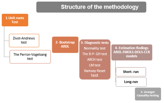
Figure 2.
Structure of the methodology.
4. Empirical Results and Discussion
The results of the Zivot–Andrews unit root test and Perron–Vogelsang unit root with one BD are reported in Table 1 and Table 2, respectively; these unit root tests suggest one and two BDs in the variables. It was revealed by these unit root tests that all the tested variables were non-stationary at level, but were stationary at the first difference. The results of the Zivot–Andrews and Perron–Vogelsang unit root tests show that the variables had one order of integration. Thus, it is more likely that Equation (1) can be used as an acceptable model of cointegration.

Table 1.
Zivot–Andrews test results.
Table 2.
The Perron–Vogelsang test results.
The findings of the bootstrap ARDL bounds test of cointegration are provided in Table 3. The findings indicate there was co-integration among ,lnGDP. Furthermore, the results of the BHT are presented in Table 4. The findings indicate that the values of the computed F-statistics exceeded the F-statistics in “EGT-JOT” and “EGT-JOT- BOT-BAT” at the 5% significance level. The results of the HJ (2008) cointegration test included two SBDs, as shown in Table 5. The results showed that the estimated statistics exceeded the 5% critical value. Therefore, the results provide evidence to reject the null hypothesis (no cointegration) at the 5% significance level.
Table 3.
The results of the bootstrap Autoregressive Distributed Lag model approach.
Table 4.
Results of the Bayer and Hanck test.
Table 5.
Results of the Hatmi-J (2008) cointegration test with two break dates.
These results provide evidence that there is a cointegration of all the variables, and confirm the results of the ARDL bound test.
The long-term coefficients were estimated through the ARDL, FMOLS, DOLS, and CCR models in Table 6. The coefficient of GDP was positive and GDP² was negative and both were significant. These findings are in line with the inverted U-shaped EKC hypothesis. Thus, these results show that the EKC is valid in Turkey, which suggests that as the level of production increases, after a certain threshold, it will lead to environmental degradation. These results are in line with [25].
Table 6.
Long-run coefficients, ARDL, DOLS, FMOLS, and CCR models.
Non-renewable energy coefficients were positively significant. Thus, it suggests that a further increase in non-renewable energy consumption will lead to further environmental pollution in Turkey. These findings are in agreement with [28] and [1]. The coefficient of renewable energy was negative and significant for Turkey, which is in line with [23]. The results suggest that an increase in alternative energy consumption will reduce climate change, thus lowering environmental pollution. Furthermore, the empirical findings show that oil price has an inverse influence on the level of carbon emissions in Turkey in both the short- and long-run. These findings are in line with [19].
The ECM model to estimate the short-run coefficients and the speed of adjustment is estimated in Equation (4). The ECM model results are presented in Table 7. They suggest that moves to its long-run equilibrium through the short-term channels by 31.1 percent speed of adjustment. The short-term coefficient of non-renewable energy was positive and significant for Turkey. However, the short-term coefficients of renewable energy were negative and significant.
Table 7.
Short-run coefficients estimates of ARDL.
The outcomes of the diagnostic tests are presented in Table 8. The normality test results showed that the p-value exceeded the 5% significance level, and it provides evidence that the model of this article is normally distributed. Furthermore, the results of the LM test indicate that there is no autocorrelation in the tested model, and this model is homoscedastic. Furthermore, the Ramsey–Reset test results suggest that the model is well specified. Figure 3 and Figure 4 show the CUSUM and CUSUM of squares (CUSUMSQ) charts. The CUSUM chart suggests that the model in this article is not mis-specified, and the CUSUM of squares shows that there was no structural change in the model over the investigated period.
Table 8.
Diagnostic test results for ARDL.
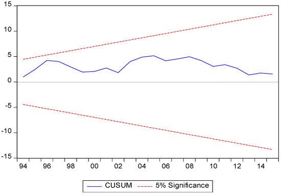
Figure 3.
Stability test using CUSUM.
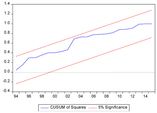
Figure 4.
Stability test using CUSUMQ.
The calculated t-statistics of the lagged value of the ECT indicates that there is a long-run causality from the oil price, renewable and non-renewable energy consumption, and economic growth on Turkey’s carbon emissions (OP, GDP, GD, REC, NREC→). The tabulated (F)statistics values (Table 9) indicate that there is a unidirectional causal relationship from oil price, economic growth, non-renewable, and renewable energy consumption to Turkey’s carbon emissions (OP, GDP, GD, REC, NREC→C). Furthermore, there is a unidirectional causal relation from the oil price to Turkey’s renewable (REC) and non-renewable energy consumption (oil, gas and coal consumption), and GDP (OP→GDP, REC, NREC). Thus, this result confirms that oil prices have a powerful influence on Turkey’s carbon emissions through GDP and non-renewable energy consumption factors. Despite the advantages of renewable energy resources in Turkey such as the lower emissions of pollutants into the atmosphere, and the fact that they cannot be depleted, non-renewable consumption of energy in Turkey has consistently increased in line with the growth in its population. In this regard, the gas consumption in Turkey has increased from 1000 million cubic feet in 1980 to 1,720,759 million cubic feet in 2014. The coal consumption in Turkey has increased from 20,530,547 tons in 1980 to 106,463,304 tons in 2014. The oil consumption in Turkey has increased from 313,200 barrels per day (B/d) in 1980 to 762,532 barrels per day (B/d) in 2014. However, the country is one of the leading global producers of textiles, ships, motor vehicles, consumer electronics, home appliances, construction materials, and other transportation equipment, which all contribute to the increasing consumption of energy from fossil fuels like oil, gas, and coal. On the other hand, Turkey is heavily dependent on imported oil, gas, and coal; more than 50% of the energy requirement has been supplied by imports. Hence, oil price fluctuations have severe effects on Turkey’s economic performance, which in turn has a negative effect on oil, coal, and gas energy consumption. Hence, our study suggests that any increase in the global oil price may cause markets or individual consumers in Turkey to postpone purchases of energy-intensive equipment that use oil, gas, and coal sources until there is greater certainty about energy costs, with a resulting reduction in the demand for equipment, capital goods, and consumer durables. Hence, an increase in oil prices may cause a shock to the supply side and accordingly reduce potential output. Furthermore, an increase in oil prices will affect consumer consumption options by shifting toward more renewable alternatives such as wind, solar, geothermal, biomass, and waves, which will in turn lead to an increase in renewable energy consumption and a decrease in oil, gas, and coal consumption, thus lowering CO2 emissions.
Table 9.
Results of the Granger causality test.
The findings of this study, namely, the positive impact of oil, gas, and coal consumption on CO2 emissions, the negative impact of renewable consumption on CO2 emissions, the negative impact of oil prices on emissions, a unidirectional causal relation from the oil price to Turkey’s non-renewable energy consumption (oil, gas, and coal consumption) are important for the policy makers in Turkey in terms of diversifying their energy mix by shifting toward more renewable alternatives, which can lead to a decrease in the carbon emissions in the country. The study suggests that the rate of imported oil in Turkey must be decreased by finding more renewable energy sources for the energy supply formula to avoid any undesirable effects of oil price fluctuations on the environmental population and also to achieve sustainable development.
5. Conclusions
This study aimed to test the effect of oil price, renewable and non-renewable energy consumption, and the GDP on carbon emissions for Turkey using the environmental Kuznets curve (EKC) model for the period between 1985 and 2015. To provide new empirical evidence, the research used the newly-developed bootstrap autoregressive distributed lag (ARDL) testing technique as proposed by (McNown et al. 2018); the newly-developed combined co-integration of Bayer and Hanck; combined co-integration as proposed Bayer and Hanck (2013); and the Hatemi-J (2012) co-integration test with two structural breaks to provide strong evidence that the co-integration was valid between the tested variables. The ARDL integration technique, DOLS, FMOLS, and CCR testing models were used to test the long-run interaction between the variables. The Granger causality (GC) analysis was applied to investigate the direction of the causal interaction among the tested variables.
The findings from ARDL, FMOL, CCR, and DOLS showed that the oil price coefficients had an inverse influence on carbon emissions in Turkey in both the short- and long-run. Furthermore, the Granger causality findings demonstrated that there was a unidirectional causal interaction from the oil price → renewable and non-renewable energy consumption, and GDP in Turkey (OP→GDP, REC, NREC). Thus, this result confirms that oil prices have a powerful influence on Turkey’s carbon emissions through GDP and nonrenewable energy consumption factors. These empirical findings can be attributed to the fact that Turkey is heavily dependent on imported oil; more than 50% of the energy requirement is satisfied by imports. Hence, the oil price fluctuations have severe effects on Turkey’s economic performance, which in turn affects the energy consumption and carbon emissions. The study suggests that the rate of imported oil in Turkey must be decreased by finding more renewable energy sources for the energy supply formula to avoid any undesirable effects of oil price fluctuations on the environmental population and also to achieve sustainable development.
Additionally, the results from ARDL, FMOL, CCR, and DOLS showed that the coefficients of the GDP were positive and the quadratic GDP was negative. These results suggest that the EKC hypothesis is valid in Turkey. The non-renewable energy coefficient was positively significant. Therefore, it could be suggested that a further increase in non-renewable energy consumption will lead to further environmental pollution in Turkey. However, the renewable energy coefficient was significant for Turkey, meaning that an increase in alternative energy consumption will reduce climate change, thus reducing environmental pollution. Turkey is one of the leading producers in the world of textiles, ships, motor vehicles, consumer electronics, home appliances, construction materials, and other transportation equipment, which all contribute to the increasing energy consumption, namely, oil, gas, and coal. On the other hand, Turkey is significantly dependent on imported oil, gas and coal; more than 50% of the energy requirement is supplied by imports. Hence, the oil price fluctuations have severe effects on economic performance in Turkey, which in turn negatively affects oil, coal, and gas energy consumption. Hence, any increase in the global oil price may cause markets or individual consumers in Turkey to postpone purchases of energy-intensive equipment that use oil, gas, and coal sources until there is greater certainty about energy costs, with a resulting reduction in demand for equipment, capital goods, and consumer durables. Thereby, an increase in oil prices may cause a shock to the supply side and accordingly reduce potential output, which in turn will lead to a reduction in oil, gas, and coal consumption, and CO2 emissions. This study provides highly important findings for policy makers in terms of diversifying the energy mix by shifting toward more renewable alternatives, which can lead to a decrease in the carbon emissions in Turkey. Hence, the study suggests that the rate of imported oil in Turkey must be decreased by finding more renewable energy sources for the energy supply formula to avoid any undesirable effects of oil price fluctuations on the environmental population, and also to achieve sustainable development. Therefore, considering the challenges of non-renewable sources (gas, oil, and coal) on the increased CO2 emissions and the environment, legislative and practical reforms could be undertaken to replace oil, gas, and coal energy sources with renewable ones. Furthermore, to increase and support the use of renewable energy sources and effectively implement the aforementioned measures, the government of Turkey should implement policies to decrease the costs of renewable resources, increase the role of green energy, and reduce its non-renewable energy consumption.
Finally, the findings of this research are important for oil-importing and exporting countries in terms of diversifying their energy mix by shifting toward more renewable alternatives. These findings are in agreement with the study of [10], which suggested that an increase in oil prices negatively affects current account balance and economic growth and other economic variables in oil-importing countries, which in turn negatively affects oil, coal, and gas energy consumption, and CO2 emissions. In contrast, an increase in oil prices positively affects current account balance and economic growth, and other economic variables in oil-exporting countries, which in turn leads to an increase in investments and non-renewable energy consumption. Therefore, the oil-importing and exporting countries need to promote the development and consumption of renewable energy so that the government can support the investments of renewable energy in the markets, which can lead to a decrease in carbon emissions. Further research for oil-importing and exporting countries is suggested for comparison purposes, not only via time series models, but panel data can also be adapted in further research to examine the nexus between oil price, energy consumption, and CO2 emissions.
Author Contributions
Project administration, supervision, M.A. (Mehmet Aga); methodology and writing-original draft preparation, investigation, data curation, formal analysis and validation review, and editing, M.A. (Mohammed Abumunshar), and A.S. All authors have read and agreed to the published version of the manuscript.
Funding
This research received no external funding
Conflicts of Interest
The authors declare no conflict of interest.
References
- Samour, A.; Isiksal, A.Z.; Resatoglu, N.G. Testing the impact of banking sector development on turkey’s (CO2) emissions. Appl. Ecol. Environ. Res. 2019, 17, 6497–6513. [Google Scholar] [CrossRef]
- McNown, R.; Sam, C.Y.; Goh, S.K. Bootstrapping the autoregressive distributed lag test for cointegration. Appl. Econ. 2018, 50, 1509–1521. [Google Scholar] [CrossRef]
- Cevik, N.K.; Cevik, E.I.; Dibooglu, S. Oil Prices, Stock Market Returns and Volatility Spillovers: Evidence from Turkey. J. Policy Model. 2020, 42, 597–614. [Google Scholar] [CrossRef]
- Etokakpan, M.U.; Adedoyin, F.; Vedat, Y.; Bekun, F.V. Does globalization in Turkey induce increased energy consumption: Insights into its environmental pros and cons. Environ. Sci. Pollut. Res. 2020, 27. [Google Scholar] [CrossRef]
- Turhan, Ş.; Garad, A.M.K.; Hançerlioğulları, A.; Kurnaz, A.; Gören, E.; Duran, C.; Aydın, A. Ecological assessment of heavy metals in soil around a coal-fired thermal power plant in Turkey. Environ. Earth Sci. 2020, 79, 1–5. [Google Scholar] [CrossRef]
- Available online: http://www.turkstat.gov.tr (accessed on 1 September 2020).
- Lardic, S.; Mignon, V. The impact of oil prices on GDP in European countries: An empirical investigation based on asymmetric cointegration. Energy Policy 2006, 34, 3910–3915. [Google Scholar] [CrossRef]
- Rafiq, S.; Salim, R.; Bloch, H. Impact of crude oil price volatility on economic activities: An empirical investigation in the Thai economy. Resour. Policy 2009, 34, 121–132. [Google Scholar] [CrossRef]
- Gorus, M.S.; Ozgur, O.; Develi, A. The relationship between oil prices, oil imports and income level in Turkey: Evidence from Fourier approximation. OPEC Energy Rev. 2019, 43, 327–341. [Google Scholar] [CrossRef]
- Rahman, S.; Serletis, A. Oil Prices and the Stock Markets: Evidence from High Frequency Data. Energy J. 2019, 40. [Google Scholar] [CrossRef]
- Mohammed Suliman, T.H.; Abid, M. The impacts of oil price on exchange rates: Evidence from Saudi Arabia. Energy Explor. Exploit. 2020, 38, 2037–2058. [Google Scholar] [CrossRef]
- Li, K.; Fang, L.; He, L. How population and energy price affect China’s environmental pollution? Energy Policy 2019, 129, 386–396. [Google Scholar] [CrossRef]
- Agbanike, T.F.; Nwani, C.; Uwazie, U.I.; Anochiwa, L.I.; Onoja, T.G.C.; Ogbonnaya, I.O. Oil price, energy consumption and carbon dioxide (CO2) emissions: Insight into sustainability challenges in Venezuela. Lat. Am. Econ. Rev. 2019, 28, 8. [Google Scholar] [CrossRef]
- Apergis, N.; Payne, J.E. Renewable energy, output, carbon dioxide emissions, and oil prices: Evidence from South America. Energy Sources Part B Econ. Plan. Policy 2015, 10, 281–287. [Google Scholar] [CrossRef]
- Alshehry, A.S.; Belloumi, M. Energy consumption, carbon dioxide emissions and economic growth: The case of Saudi Arabia. Renew. Sustain. Energy Rev. 2015, 41, 237–247. [Google Scholar] [CrossRef]
- Simsek, T.; Yigit, E. Causality Analysis of BRICT Countries on Renewable Energy Consumption, Oil Prices, CO2 Emissions, Urbanization and Economic Growth. Eskişehir Osman. Univ. J. Econ. Adm. Sci. 2017, 12, 117–136. [Google Scholar]
- Zhao, Y.; Zhang, Y.; Wei, W. Quantifying international oil price shocks on renewable energy development in China. Appl. Econ. 2020, 1–16. [Google Scholar] [CrossRef]
- Malik, M.Y.; Latif, K.; Khan, Z.; Butt, H.D.; Hussain, M.; Nadeem, M.A. Symmetric and asymmetric impact of oil price, FDI and economic growth on carbon emission in Pakistan: Evidence from ARDL and non-linear ARDL approach. Sci. Total. Environ. 2020, 726, 138421. [Google Scholar] [CrossRef]
- Katircioglu, S. Investigating the role of oil prices in the conventional EKC model: Evidence from Turkey. Asian Econ. Financ. Rev. 2017, 7, 498–508. [Google Scholar] [CrossRef]
- Zou, X. VECM Model Analysis of Carbon Emissions, GDP, and International Crude Oil Prices. Discret. Dyn. Nat. Soc. 2018, 2018, 1–11. [Google Scholar] [CrossRef]
- Pao, H.T.; Tsai, C.M. Modeling and forecasting the CO2 emissions, energy consumption, and economic growth in Brazil. Energy 2011, 36, 2450–2458. [Google Scholar] [CrossRef]
- Bölük, G.; Mert, M. The renewable energy, growth and environmental Kuznets curve in Turkey: An ARDL approach. Renew. Sustain. Energy Rev. 2015, 52, 587–595. [Google Scholar] [CrossRef]
- Magazzino, C. The relationship among real GDP, CO2 emissions, and energy use in South Caucasus and Turkey. Int. J. Energy Econ. Policy 2016, 6, 672–683. [Google Scholar]
- Bento, J.P.C.; Moutinho, V. CO2 emissions, non-renewable and renewable electricity production, economic growth, and international trade in Italy. Renew. Sustain. Energy Rev. 2016, 55, 142–155. [Google Scholar] [CrossRef]
- Bilgili, F.; Koçak, E.; Bulut, Ü. The dynamic impact of renewable energy consumption on CO2 emissions: A revisited Environmental Kuznets Curve approach. Renew. Sustain. Energy Rev. 2016, 54, 838–845. [Google Scholar] [CrossRef]
- Shafiei, S.; Salim, R.A. Non-renewable and renewable energy consumption and CO2 emissions in OECD countries: A comparative analysis. Energy Policy 2014, 66, 547–556. [Google Scholar] [CrossRef]
- Chen, W.; Geng, W. Fossil energy saving and CO2 emissions reduction performance, and dynamic change in performance considering renewable energy input. Energy 2017, 120, 283–292. [Google Scholar] [CrossRef]
- Dogan, E.; Ozturk, I. The influence of renewable and non-renewable energy consumption and real income on CO2 emissions in the USA: Evidence from structural break tests. Environ. Sci. Pollut. Res. 2017, 24, 10846–10854. [Google Scholar] [CrossRef]
- Park, J.Y. Canonical cointegrating regressions. Econom. Soc. 1992, 60, 119–143. [Google Scholar] [CrossRef]
- Corizzo, R.; Ceci, M.; Fanaee-T, H.; Gama, J. Multi-aspect renewable energy forecasting. Inf. Sci. 2020, 546, 701–722. [Google Scholar] [CrossRef]
- Bessa, R.J.; Möhrlen, C.; Fundel, V.; Siefert, M.; Browell, J.; Haglund El Gaidi, S.; Kariniotakis, G. Towards improved understanding of the applicability of uncertainty forecasts in the electric power industry. Energies 2017, 10, 1402. [Google Scholar] [CrossRef]
- Ceci, M.; Corizzo, R.; Malerba, D.; Rashkovska, A. Spatial autocorrelation and entropy for renewable energy forecasting. Data Min. Knowl. Discov. 2019, 33, 698–729. [Google Scholar] [CrossRef]
- Zivot, E.; Andrews, D.W.K. Further evidence on the great crash, the oil-price shock, and the unit-root hypothesis. J. Bus. Econ. Stat. 2002, 20, 25–44. [Google Scholar] [CrossRef]
- Perron, P.; Vogelsang, T.J. A note on the asymptotic distributions of unit root tests in the additive outlier model with breaks. Braz. Rev. Econ. 1993, 13, 8l–20l. [Google Scholar]
- Pata, U.K. Environmental Kuznets curve and trade openness in Turkey: Bootstrap ARDL approach with a structural break. Environ. Sci. Pollut. Res. 2019, 26, 20264–20276. [Google Scholar] [CrossRef] [PubMed]
- Pesaran, M.H.; Shin, Y.; Smith, R.J. Bounds testing approaches to the analysis of level relationships. J. Appl. Econ. 2001, 16, 289–326. [Google Scholar] [CrossRef]
- Bayer, C.; Hanck, C. Combining non-cointegration tests. J. Time Ser. Anal. 2013, 34, 83–95. [Google Scholar] [CrossRef]
- Engle, R.F.; Granger, C.W. Co-integration and error correction: Representation, estimation, and testing. Econom. J. Econ. Soc. 1987, 55, 251–276. [Google Scholar] [CrossRef]
- Johansen, S. Statistical analysis of cointegration vectors. J. Econ. Dyn. Control. 1988, 12, 231–254. [Google Scholar] [CrossRef]
- Boswijk, H.P. Testing for an unstable root in conditional and structural error correction models. J. Econ. 1994, 63, 37–60. [Google Scholar] [CrossRef]
- Banerjee, A.; Dolado, J.; Mestre, R. Error-correction mechanism tests for cointegration in a single-equation framework. J. Time Ser. Anal. 1998, 19, 267–283. [Google Scholar] [CrossRef]
- Hatemi-j, A. Tests for cointegration with two unknown regime shifts with an application to financial market integration. Empir. Econ. 2008, 35, 497–505. [Google Scholar] [CrossRef]
- Phillips, P.C.; Hansen, B.E. Statistical inference in instrumental variables regression with I (1) processes. Rev. Econ. Stud. 1990, 57, 99–125. [Google Scholar] [CrossRef]
- Stock, J.H.; Watson, M.W. A simple estimator of cointegrating vectors in higher order integrated systems. Econom. J. Econ. Soc. 1993, 61, 783–820. [Google Scholar] [CrossRef]
- Bessa, R.; Moreira, C.; Silva, B.; Matos, M. Handling renewable energy variability and uncertainty in power systems operation. Wiley Interdiscip. Rev. Energy Environ. 2014, 3, 156–178. [Google Scholar] [CrossRef]


Publisher’s Note: MDPI stays neutral with regard to jurisdictional claims in published maps and institutional affiliations. |
© 2020 by the authors. Licensee MDPI, Basel, Switzerland. This article is an open access article distributed under the terms and conditions of the Creative Commons Attribution (CC BY) license (http://creativecommons.org/licenses/by/4.0/).