Jump Linear Quadratic Control for Microgrids with Commercial Loads

Abstract

Due to the aging power-grid infrastructure and increased usage of renewable energies, microgrids (μGrids) have emerged as a promising paradigm. It is reasonable to expect that they will become one of the fundamental building blocks of a smart grid, since effective energy transfer and coordination of μGrids could help maintain the stability and reliability of the regional large-scale power-grid. From the control perspective, one of the key objectives of μGrids is load management using local generation and storage for optimized performance. Accomplishing this task can be challenging, however, particularly in situations where local generation is unpredictable both in quality and in availability. This paper proposes to address that problem by developing a new optimal energy management scheme, which meets the requirements of supply and demand. The method that will be described in the following models μGrids as a stochastic hybrid dynamic system. Jump linear theory is used to maximize storage and renewable energy usage, and Markov chain theory is applied to model the intermittent generation of renewable energy based on real data. Although the model itself is quite general, we will focus exclusively on solar energy, and will define the performance measure accordingly. We will demonstrate that the optimal solution in this case is a state feedback law with a piecewise constant gain. Simulation results are provided to illustrate the effectiveness of such an approach.

1. Introduction

The power industry landscape is changing rapidly, due to the emergence of Distributed Energy Resources (DERs) and new storage technologies, active demand-side participation, and the growing need for green/renewable energy. At the same time, it is clear that the grid infrastructure is aging, and that maintaining its resiliency and reliability will require significant resources. These two factors have created the need to re-examine the existing power-grid structure (which is now over 100 years old).

The proliferation of microgrids (μGrids) has been steadily growing in recent years, and this is likely to be an important part of the grid of the future. It is widely believed that the next generation of μGrids will not be used just for supplying backup power, and will also provide a complex network configuration that possesses all the essential attributes of a large-scale grid (such as the ability to balance electrical demand with sources, schedule the dispatch of resources and maintain grid reliability). It is reasonable to expect that these new μGrids will enable greater use of DERs, limit greenhouse gas emissions, improve local grid reliability and reduce operating costs [1]. We should also mention in this context that μGrids can become a potentially useful tool for managing the variability of intermittent Renewable Energy Sources (RESs) such as solar energy, due to the decreasing cost of DERs [1].

Considering that 90% of all power outages and disturbances originate in the distribution system due to component failures and load imbalances [2], and recognizing that occurrences of natural disasters have increased in the last few years [3], it is imperative to move towards a decentralized grid that allows for more flexibility and scalability. It is becoming increasingly clear that the grid of the future will involve a considerable amount of “plug and play”, in which μGrids will play an essential role (particularly when it comes to optimized interoperability) [4]. The power industry has already embarked on this path, and has considered DERs as a viable alternative to centralized generation [5].

Integration of DER units in general (and μGrids in particular) gives rise to several operational challenges, such as bidirectional power flows, potential instability, uncertainty and low inertia [6]. A considerable amount of research is currently being conducted on the design and management of μGrids, and the problems that arise when they are connected to the grid. The solutions that have been proposed so far take many different forms, and depend on how the μGrid is being used. In general, it is possible to classify these techniques into three broad categories, based on the type of problem that they consider. Some of them deal with utility μGrids (where a city district operates as a μGrid), others with commercial and industrial μGrids (such as commercial buildings, university campuses, factories, and manufacturing plants, for example) and there are also those that focus on remote μGrids (which operate only in an islanded mode) [7]. The method proposed in this paper is aimed exclusively at commercial μGrids, since there is a considerable amount of publicly available data that pertains to their load patterns.

Energy management in μGrids is usually considered to be a hierarchical control system with three levels [8,9], the first of which is known as primary control. Primary control is concerned with the interface between generators, storage devices, and loads. The control actions are based on local measurements, and must be performed quickly (often within a few milliseconds). Secondary control (which is also referred to as local energy management of individual μGrids) is responsible for correcting the errors produced by the primary control. It acts over a longer period of time, and ensures the reliable operation of μGrids. Tertiary control (which we will focus on in this paper) coordinates the operation of multiple μGrids that interact with each other, as well as with the utility grid. It regulates active and reactive power flow, and supplies secondary control units with reference voltages. By doing so, tertiary control provides an optimal power schedule which allows individual μGrids to use their resources in the most effective way.

Because standard energy management schemes for μGrids were typically based on deterministic control strategies and optimization techniques, they were not able to manage random energy generation efficiently [10,11,12,13,14,15,16,17,18,19]. In [10,11,12] decentralized control was considered to be a strategy for energy management of μGrids. A robust decentralized servomechanism controller for power management of an autonomous multi-DER was analyzed in [10], and a decentralized bi-level algorithm for energy management of networked μGrids was considered in [11]. In [12], decentralized control schemes were proposed for μGrids to maintain the desired temperature in local buildings at a minimum cost.

Reference [13] examines a centralized approach for controlling the power flow in hybrid μGrids, and [14] uses dynamic programing to control energy storage devices by solving the optimal power flow problem on the tertiary control level. State of the art of control strategies and the control challenges that they introduce for distributed energy storage systems in μGrids are discussed in [15]. Parisio et al. [16] apply model predictive control by using a mixed-integer linear programming formulation to optimize μGrids operation, while [17] considers a scenario-based robust energy management method for uncertain renewable generation and load. In this context, we should also mention references [18] and [19], which use an alternating-direction multiplier method to optimize the operation of multiple μGrids.

Although these deterministic solutions were important in the planning of μGrid resources over time, increased use of intermittent renewable energy has encouraged researchers to study μGrid energy scheduling in a stochastic framework. Several such algorithms have been developed in recent years [20,21,22,23,24,25,26], each of which takes into account the uncertainty of non-dispatchable generation and loads. It should be noted that in most of these cases, the proposed solutions rely on a stochastic programming approach, and the intermittent RESs are described using empirical data (or are modeled as Gaussian processes). In [20,21], for example, energy scheduling of μGrids with integrated RES is formulated as a stochastic problem, and a two-stage stochastic optimization is proposed for day ahead transactions and dispatching. The focus in [22] is an online energy management strategy for real-time operation of μGrids. In this paper, online energy management is modeled as a stochastic optimal power flow problem using a Lyapunov optimization algorithm. Han et al. [23] give an overview of distributed coordinated control strategies for μGrids with high integration of RES, which are based on multiagent systems. In [24,25], a hierarchical control structure is proposed which uses stochastic model predictive control for energy management of individual μGrids, and reference [26] considers a one-step method for optimizing the long term operation cost of a μGrid. An interesting feature of this method is that it does not require statistical knowledge of uncertainties in the load, the renewable energy generation or electricity prices. It is important to keep in mind that all the methods mentioned above rely on iterative techniques to find a viable solution. In that respect they are different from the approach proposed in this paper.

Papers that have used Markov processes to model random RES and battery energy storage systems are of particular interest for this study. In [27], a semi-Markov process model was proposed to model photovoltaic (PV) power and a rule-based controller was used to compute average generator and battery power during each scheduling interval. Belloni et al. [28], use Markov chains to model uncertainties in the RES generation, and propose a stochastic dynamic programming algorithm to minimize the cost of energy consumption in wind powered μGrids with energy storage system. In [29], a Markov jump process was used to model the stochastic changes in distributed energy storage systems.

In [30], a stochastic model predictive control was applied to design optimal control for wind turbines that are subject to random wind speed. The authors formulated a Markov jump linearization model to describe random switching characteristics of the wind turbine. Markov chains have also been used by Li and Roche [31] to develop a two-stage scheduling algorithm for multi-energy supply microgrids, and an online learning prediction method was introduced to anticipate the short-term load demands and renewable outputs in real-time dispatching. In a more recent work [32], a solar generation model was proposed based on the Markov chain approach, which predicts the power generation of solar cells.

From the above discussion, it is clear that energy management systems for μGrids need to be designed in a way that reduces the impact of load variations, natural disasters, and the inherent randomness of RES. The difficulty, however, is that most of the energy management strategies proposed to date use online optimization techniques that are computationally demanding and costly to implement. To address this issue, we propose an optimal control scheme which relies on a simplified model that represents multiple μGrids as multivariate stochastic hybrid dynamic systems. The controller design is based on jump linear theory, which is used to maximize storage and renewable energy usage.

It is important to recognize in this context that the proposed approach does not attempt to predict weather parameters (such as the availability of solar or wind energy, for example) on a daily basis [32,33,34]. Instead, it relies on yearly regional weather data to build a probabilistic model that is used to compute appropriate control gains offline.

The main contribution of this paper is the application of Jump Linear Quadratic Control (JLQC) to a model that combines deterministic and stochastic elements. This hybrid representation (coupled with a quadratic cost function) provides the necessary mathematical framework for optimizing the use of storage and solar energy by piecewise control action. An important feature of this control strategy is that it does not require online optimization. As a result, it is computationally efficient, and is relatively easy to implement compared to other techniques proposed in the literature. This is particularly important in cases where the system includes many interacting microgrids.

The paper is organized as follows. In Section 2, we present a simplified model for a flexible grid structure. We then proceed to develop a stochastic optimal control strategy, which is described in Section 3. Simulation results and their analysis are provided in Section 4, while Section 5 offers some conclusions (as well as a brief discussion of possible directions for future work).

2. System Description and Mathematical Modeling

We begin this section, by offering a general system description that addresses some recent challenges in power-grid energy management. We will then introduce a simple mathematical model for the grid that will allow us to develop a stochastic optimal control strategy.

2.1. The System Description

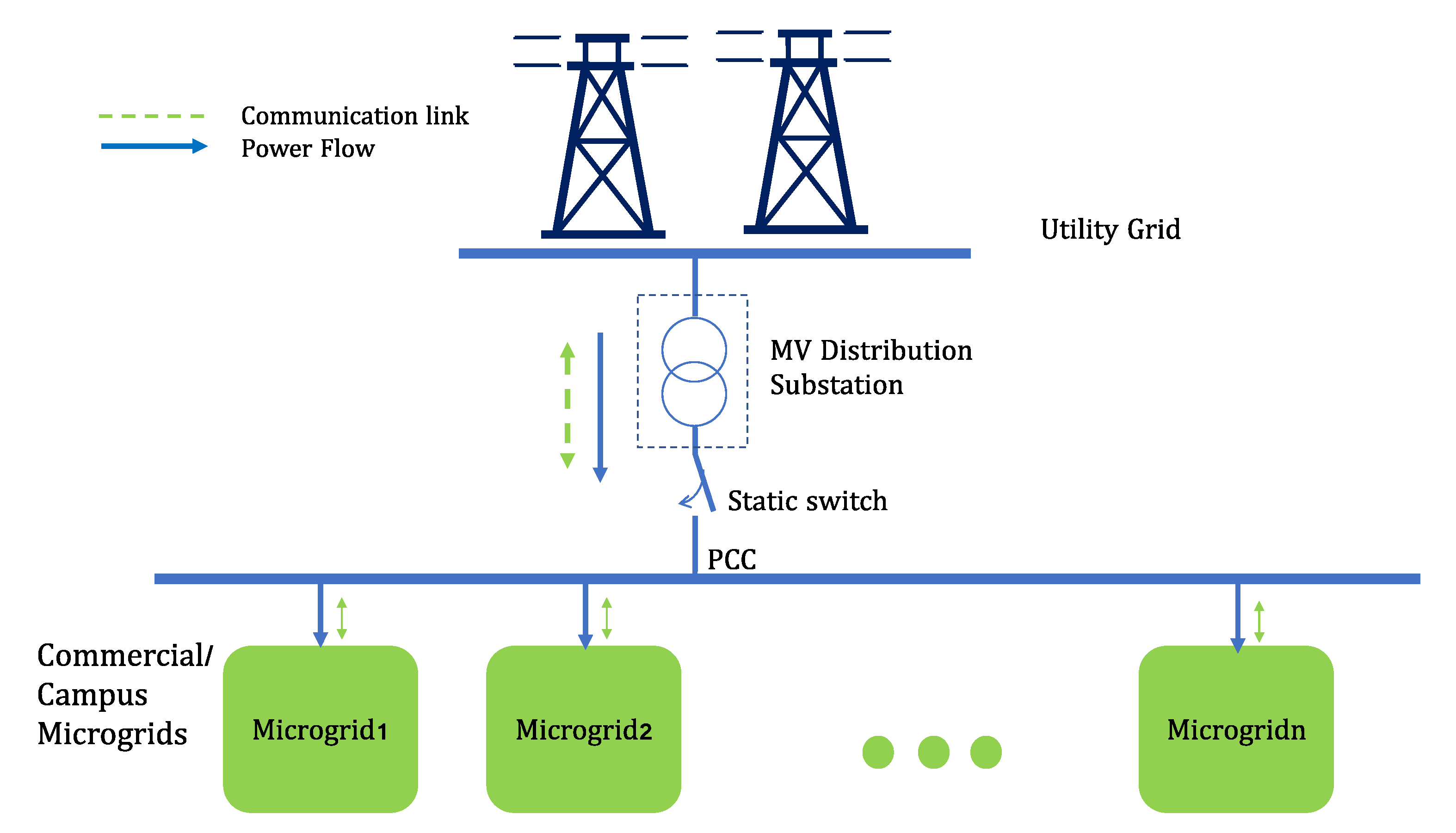
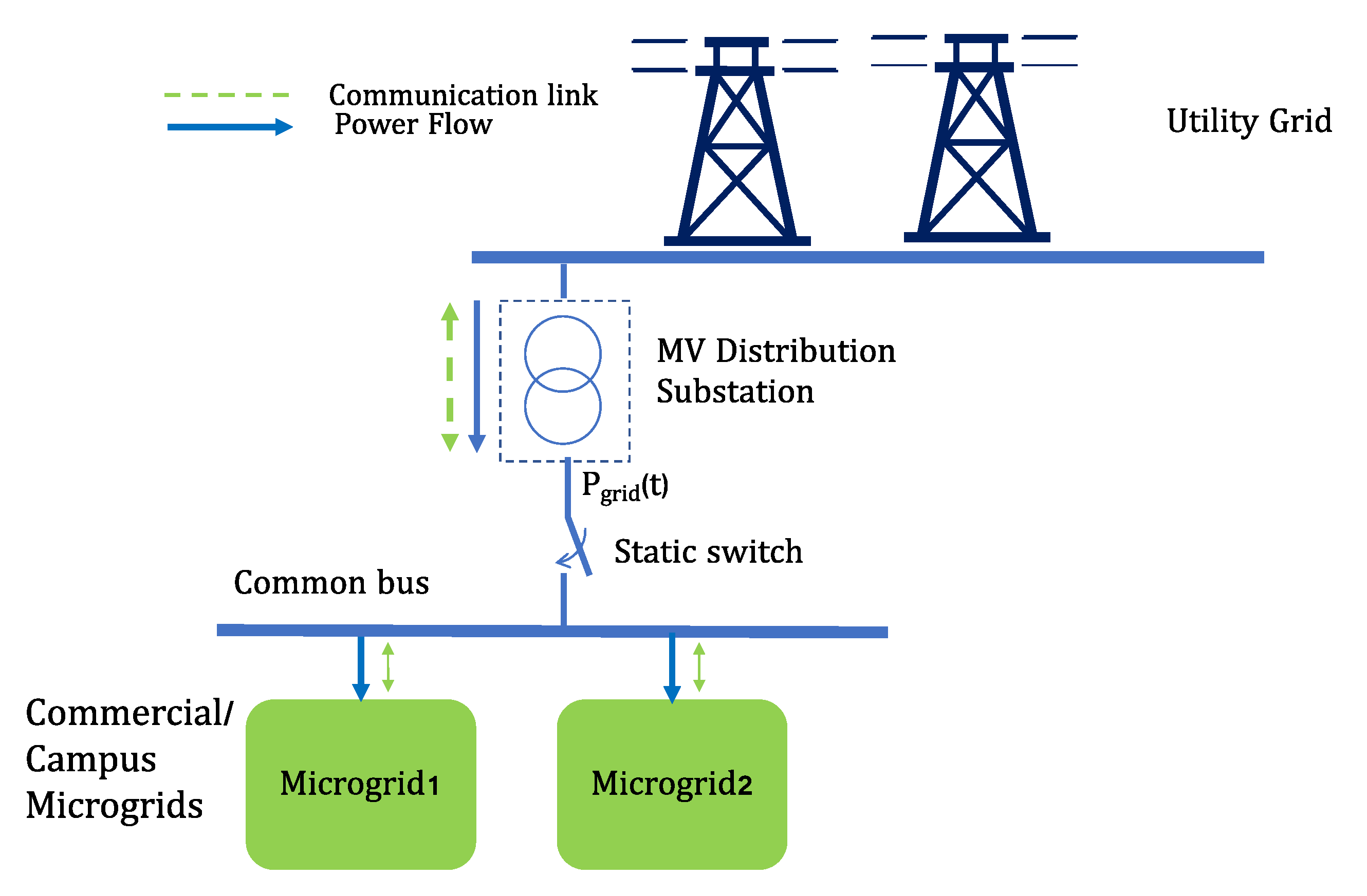
Figure 1 provides a schematic representation of multiple μGrids that can be connected to and disconnected from the utility grid via a medium voltage (MV) distribution substation. In this configuration, μGrids that are connected can be viewed as a cluster that is linked to the grid through a point of common coupling (PCC), while those that are disconnected are considered to be islanded. A continuous dynamic model for structures of this type will be proposed in the next section. Depending on the grid requirements, a communication link may exist between the grid and the μGrids for the exchange of information.

As noted in the Introduction, this study will focus on commercial μGrids (including university campuses). Systems of this sort have two important features that allow us to develop an effective and robust control strategy:

• Although each μGrid load may be comprised of multiple buildings, their aggregated power has a predictable profile
• The load demand reaches its peak during the day (when solar energy is available), and reaches its minimum at night.

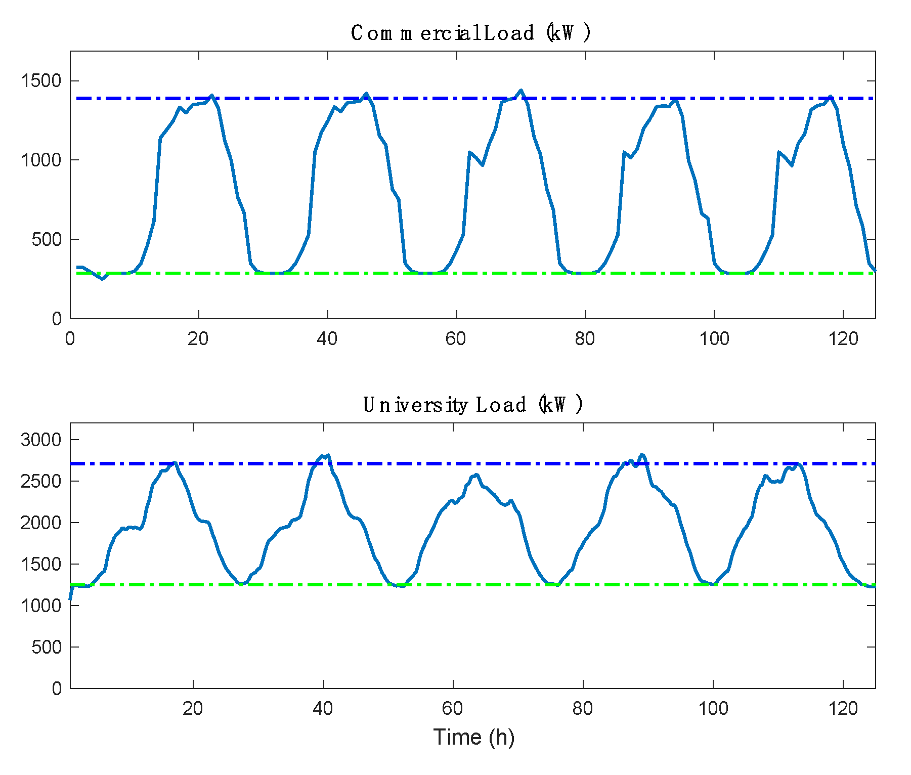
Data that validates these two points is provided in Figure 2, which shows the hourly power usage for a typical commercial load [35] and for Santa Clara University [36].

In modeling the dynamic behavior of μGrids that can operate both in the islanded mode and in the connected mode, we will not consider the possibility of bidirectional energy transfer between the utility grid and μGrids. This assumption helps prevent grid instability due to the stochastic nature of the net load, which represents the difference between the total load and the solar generation (in this instance and throughout the paper, the term “stability” is understood in the sense of Lyapunov).

Each cluster of μGrids can be connected to or disconnected from the grid in a scheduled or random manner, depending on their load and their generation needs. We will assume that islanded μGrids are controlled using only locally available information, and our objective will be to stabilize each disconnected μGrid using a stochastic optimal control law. This control law must ensure that stability (and an acceptable level of suboptimality) is retained when one or more μGrids are reconnected to the grid. Transitions of this sort are bound to occur, since μGrids are not designed to operate indefinitely in isolation.

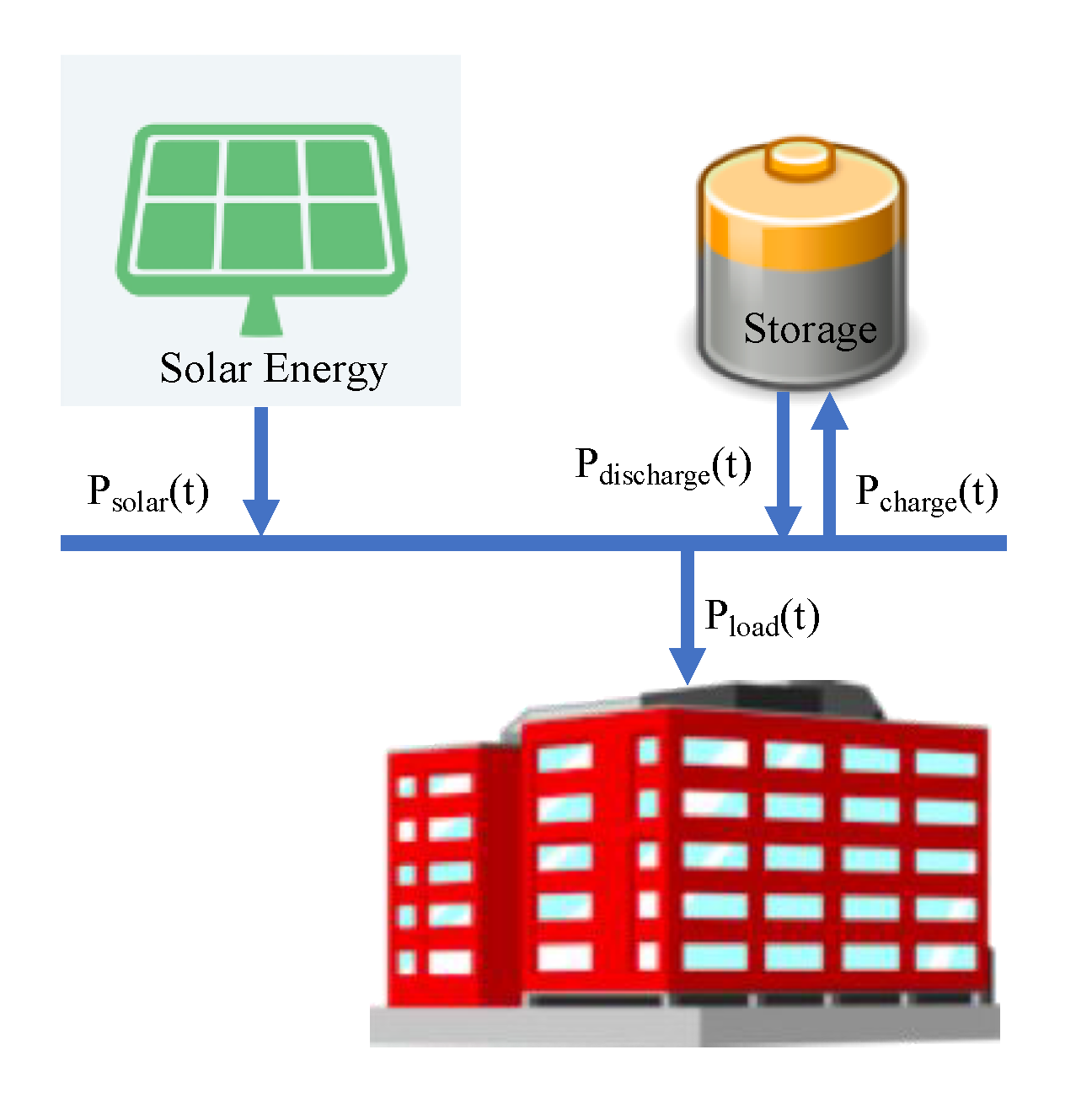
Figure 3 shows the basic structure of each μGrid, which consists of a specific load (commercial or a university campus), battery storage, and an array of solar cells. When μGrid operates in the connected mode, the utility grid provides energy both to the load and to the battery. Unused solar energy by the load may also charge the battery if needed. When it is in the islanded mode, solar energy is provided internally, and is distributed to the battery and the load in a way that reflects the load requirements. During the night, it is assumed that the battery is the sole source of energy. This is a reasonable assumption, since most large consumers require less energy during the night than during the day (see Figure 2). In situations where the required battery storage is not available, a secondary generation source (such as fuel cell, for example) may be considered. This addition has little effect on the complexity of the model and the control strategy, so we will disregard it in our analysis.

2.1.1. Load Model

In the simplified scenario that we just described, the primary goal is to manage the energy demand. This is done by ensuring that the power generated by the utility grid ($P_{grid}$), the PV array ($P_{solar}$) and the battery ($P_B$) is balanced with the power required by the load $(P_{load})$. We can express this relationship as:

$$P_{load}\left(t\right)=P_{grid}\left(t\right)+P_{solar}\left(t\right)+P_B\left(t\right).$$

(1)

It is assumed that $P_{load}\left(t\right)$ follows a preassigned trajectory, whose characteristics will be defined in the following section. $P_{solar}\left(t\right)$ (which represents the power generated by the PV array) can be viewed as the result of a stochastic process whose characteristics depend on cloud coverage as well as the time of day. Since the battery can deliver power to the load (or can absorb it when charging), we will treat $P_B\left(t\right)$ as a control input. Power losses that are mostly due to transmission lines are neglected in this model, since μGrids are considered to be sufficiently close to substations (less than 10 miles).

The PV array should be designed in a way that reflects the daytime load requirements (which is becoming increasingly feasible, due to decreasing cost of solar panels). Doing so ensures full load satisfaction when the weather is sunny, and the excess energy can be transferred to the battery. Because of that, the battery can act as a buffer, which allows the system to use the stored solar energy when the PV array is inactive.

In addition to the relationship described in (1), our model incorporates the following three assumptions:

• Information about the system state is readily available, including instantaneous power flow, acceptable limits for generation levels, and maximum and minimum battery levels. This can be ensured by using a State of Charge (SoC) tracker for the battery, in conjunction with voltage, current, or phasor monitoring devices.
• Only active power is considered, and voltages and phase angles are assumed to be regulated by controllers/inverters on the PV array and the battery.
• The load for each μGrid conforms to the pattern provided in the National Renewable Energy Laboratory (NREL) System Advisor Model (SAM) dataset. This data can be found online [35], and represents the “average” commercial load in the United States.

2.1.2. Solar Generation Model

Although solar power is clearly a desirable form of generation (because of its passive generation profile and the decreasing cost of panels), it has certain intrinsic shortcomings which stem from its intermittent nature. The most important one is that PV generation requires sunny weather for maximal efficiency, which means that generation can be severely impacted by heavy cloud coverage. To model the stochastic nature of solar generation, we will use a continuous Markov chain to describe cloud coverage patterns (following the methodology proposed in [37]).

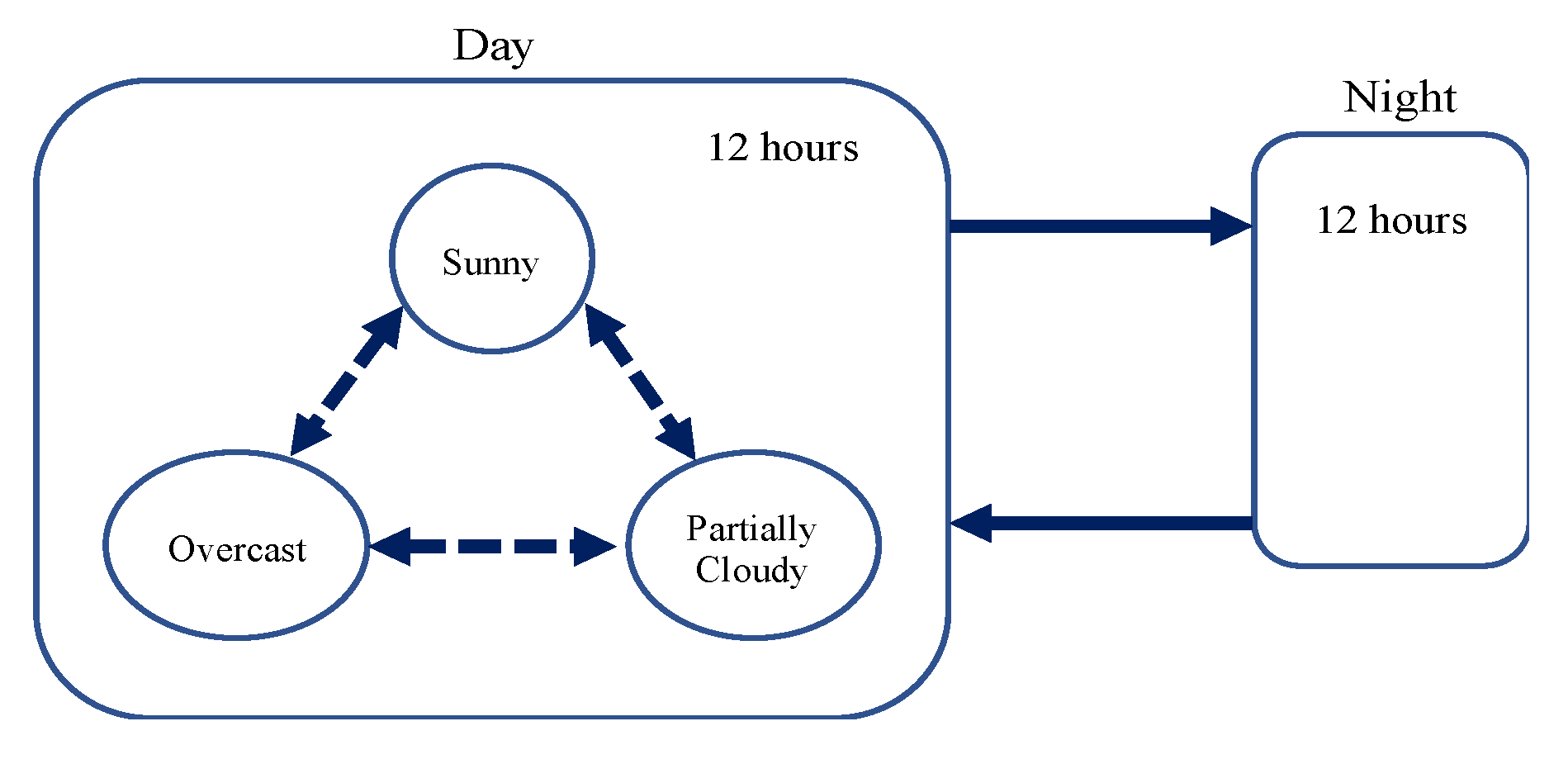
In general, cloud coverage classification should be based on regional weather patterns. As shown in Figure 4, in northern California, the level of cloud coverage during the day can be classified as sunny, partially cloudy, and overcast. Since there is no solar generation at night, the power generated by the PV array can be represented as a piecewise constant function:

$$P_{solar}\left(t\right)=\{\begin{array}{l}{P}_{solar}\left(r(t\right)) with r\left(t\right)=\{\begin{array}{c}1 \left(\mathrm{sunny}\right)\\ 2 \left(\mathrm{partially} \mathrm{cloudy}\right)\\ 3 \left(\mathrm{overcast}\right)\end{array}\hfill \\ 0 during night\hfill \end{array}.$$

(2)

The actual values that $P_{solar}\left(r\left(t\right)\right)$ takes depend on the number of panels, efficiency, and the cloud coverage.

The term $r\left(t\right)$ that appears in (2) represents the mode of the Markov chain that corresponds to the level of cloud coverage. This means that r(t) evolves according to a continuous time Markov chain, and is restricted to three possible values. The transition probability matrix P indicating the probability $p_{ij}$ of transitioning from state i to state j, $P=\left\{p_{ij}\right\}$ is given by:

$$\begin{gathered} p_{ij}=Prob\left(r\left(t+∆\right)=j|r\left(t\right)=i\right)={\pi }_{ij}\mathsf{∆}+o\left(\mathsf{∆}\right) \mathrm{if} i\ne j \\ =1+{\pi }_{ii}\mathsf{∆}+o\left(\mathsf{∆}\right) \mathrm{if} i=j \end{gathered}$$

(3)

where $∆>0$ and $\underset{∆\to 0}{\lim }\frac{0(∆)}{∆}=0$. Coefficients ${\pi }_{ij}$ represent the (non-negative) transition rate from i to j ($i\ne j)$, and ${\pi }_i$ is defined as

$${\pi }_i\triangleq -{\pi }_{ii}\triangleq {\displaystyle \sum }_{j=1, j\ne i}^3{\pi }_{ij}.$$

(4)

Given this notation, the transition rate matrix $\Pi$ will have the form $\Pi =({\pi }_{ij}) \left(i,j=1,2,3\right)$ [38].

Data for the cloud coverage transition probability matrix was obtained from San Jose International Airport’s meteorological reports [39], (also known as METAR). This data contains information about precipitation and cloud coverage, and is routinely collected at all major airports and government buildings in the United States. For the purposes of our study the hourly cloud coverage data was “quantized” in a way that differentiates between three levels: sunny, partially cloudy, and overcast. The transition probability and the transition rates were calculated using this data set (which contains information gathered between 2008 and 2017).

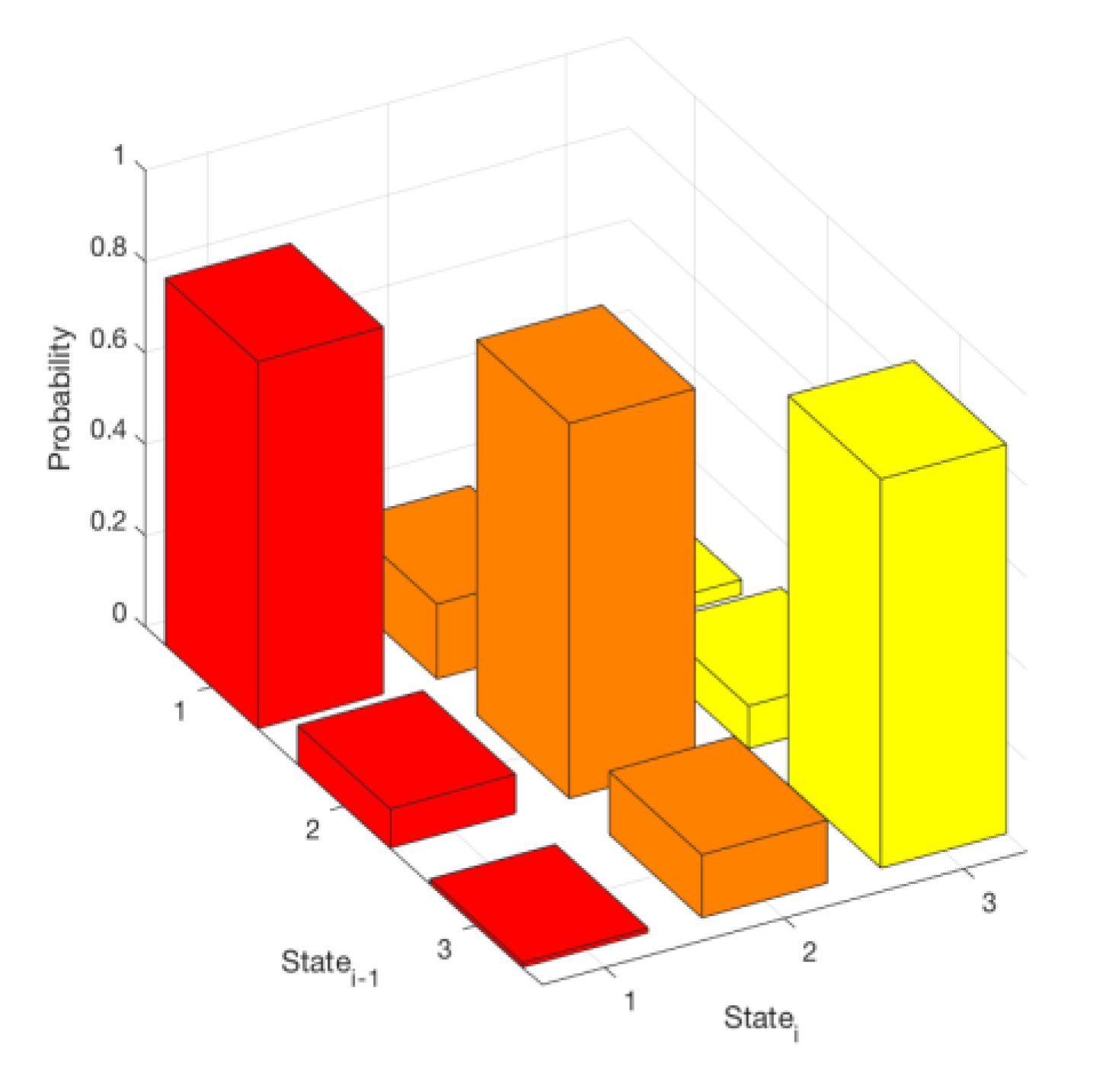
The data analysis confirmed that the transition probability from one state to the other state does not change significantly from year to year. The transition probability matrix obtained for 2016 is shown in Figure 5. It is interesting to note how the magnitudes on the main diagonal compare to the off-diagonal elements in the transition matrix. It is evident that the cloud coverage tends to remain in one state for prolonged periods of time. These long stretches of continuous weather are clearly consistent with California’s stable weather patterns.

2.1.3. Battery Model

Battery energy storage systems are commonly used to supplement generation from the PV array, (which is inherently intermittent). Relevant battery characteristics include its energy capacity (more specifically SoC), discharge/charge powers, safe operating temperatures, and life cycle. The SoC of a battery represents its available capacity expressed as a percentage of its rated capacity. Since depleting or overcharging the battery can have detrimental effects, the SoC of the battery should always be maintained within proper limits. Voltage and current measurements can be used to estimate SoC, since they cannot be measured directly. In the following, we will assume that the energy stored in the battery, E_B(t), and the charge power P_B(t) can be used to provide adequate information about the SoC. The battery energy storage has the following limits, $E_{Bmin}\le E_B\left(t\right)\le E_{Bmax}$, as well as discharging and charging limits, $0\le P_B^{dis.}\left(t\right)\le {\overline{P}}_B^{dis.}, 0\le P_B^{ch.}\left(t\right)\le {\overline{P}}_B^{ch.}$. In the second and third inequality, ${\overline{P}}_B^{ch.} \mathrm{and} {\overline{P}}_B^{dis.}$ represent the maximal allowable charge and discharge values, respectively.

Variations in the energy stored in the battery can be expressed as [14]

$$\frac{d{E}_B\left(t\right)}{dt}=P_B^{ch.}\left(t\right)-P_B^{dis.}\left(t\right)-\gamma E_B\left(t\right)$$

(5)

where $P_B^{ch.}=P_{solar}\left(t\right)+P_{grid}\left(t\right)$, and $\gamma$ denotes the rate of self-discharge. We will assume that batteries have the same efficiency when charging and discharging, and that they can do so concurrently. This feature becomes important in cases when μGrids exchange energy directly. To ensure normal battery operation (and increase its lifespan), it is standard practice to maximize the lifespan of the battery by setting $E_{Bmin}\ge 10\%$ and $E_{Bmax}\le 90\%$ of the maximum energy that can be stored.

2.2. Simplified Mathematical Model

A simplified model that describes the energy management of a single μGrid in an n μGrid system has the form:

$$\begin{array}{c}\frac{d{E}_{Bm}}{dt}\left(t\right)=\left(1-{\alpha }_m\right)P_{solarm}\left(t\right)+\left(1-{\beta }_m\right)P_{gridm}\left(t\right)-P_{discm}\left(t\right)-{\gamma }_m{E}_{Bm}\left(t\right)\\ P_{Lm}\left(t\right)={\alpha }_m{P}_{solarm}\left(t\right)+{\beta }_m{P}_{gridm}\left(t\right)+P_{discm}\left(t\right)\end{array} \mathrm{with} m=1$$

(6)

In (6), $E_{Bm}$ represents energy stored in battery m, $P_{Lm}$ is the load demand of μGrid m, $P_{solarm}$ denotes solar power generated for μGrid m, and $P_{gridm}$ is the amount of power delivered from the utility grid to μGrid m. The quantity $P_{discm}$ represents the power delivered from the battery to the load. Parameter ${\alpha }_m$ is the fraction of solar power delivered to load m, and ${\beta }_m$ is the fraction of power delivered from the main grid to μGrid m (it is assumed that any unused energy is absorbed by the battery). The values of these two constants are chosen based on the solar panel size and battery storage capacity.

Coefficient ${\gamma }_m$ denotes the rate of self-charge for battery m, and $P_{grid}\left(t\right)$ is the power allocated by the utility grid for the n μGrids. This power can be expressed as

$$P_{grid}\left(t\right)=P_{grid1}\left(t\right)+P_{grid2}\left(t\right)+\cdots +P_{gridn}\left(t\right)$$

(7)

and can be bounded as $0\le P_{grid}\left(t\right)\le P_G^M$. To balance the power in the network, $P_{gridm}$ must satisfy

$$P_{gridm}\left(t\right)=P_{grid}\left(t\right)-\psi E$$

(8)

where vector $\psi =[{\theta }_{mp}]$ represents the tuning coefficients for μGrid m and component p (which can be a battery or a load). Vector $E={\left[E_{Bl}\left(t\right), E_{Ll}\left(t\right)\right]}^T, \left(l=1,\dots ,n; l\ne m\right),$ consists of components $E_{Bl} \mathrm{and} E_{Ll}$, which denote the energy stored in battery l and the energy absorbed by load l, respectively.

In the state space, the mathematical model described above can be represented as

$$\{\begin{array}{c}\dot{x}\left(t\right)=\left(\begin{array}{ccc}{A}_{11}& \cdots & A_{1n}\\ ⋮& \ddots & ⋮\\ A_{n1}& \cdots & A_{nn}\end{array}\right)x\left(t\right)+\left(\begin{array}{cc}\begin{array}{cc}{B}_1& \cdots \end{array}& 0\\ \begin{array}{cc}⋮& \ddots \end{array}& ⋮\\ \begin{array}{cc}0& \cdots \end{array}& B_n\end{array}\right)u\left(t\right)+P\left(t\right)\\ y\left(t\right)=\left(\begin{array}{ccc}1& \cdots & 0\\ ⋮& \ddots & ⋮\\ 0& \cdots & 1\end{array}\right)x\left(t\right)\end{array}$$

(9)

with

$$A_{mm}=\left(\begin{array}{cc}-{\gamma }_m& 0\\ 0& 0\end{array}\right),A_{ml}=\left(\begin{array}{c}-\left(1-{\beta }_m\right){\theta }_{mm}\begin{array}{cc}\cdots & -\left(1-{\beta }_m\right){\theta }_{ml}\end{array}\\ -{\beta }_m{\theta }_{mm}\begin{array}{cc}\cdots & -{\beta }_m{\theta }_{ml}\end{array}\end{array}\right),B_m=\left(\begin{array}{c}-1\\ 1\end{array}\right),$$

$$x=\left[\begin{array}{c}{x}_1\\ \begin{array}{c}{x}_2\\ \begin{array}{c}⋮\\ x_{2n}\end{array}\end{array}\end{array}\right]=\left[\begin{array}{c}{E}_{B1}\\ \begin{array}{c}{E}_{L1}\\ \begin{array}{c}\begin{array}{c}⋮\\ E_{Bn}\end{array}\\ E_{Ln}\end{array}\end{array}\end{array}\right], u=\left[\begin{array}{c}{u}_1\\ \begin{array}{c}\begin{array}{c}{u}_2\\ ⋮\end{array}\\ u_n\end{array}\end{array}\right]=\left[\begin{array}{c}{P}_{disc1}\\ \begin{array}{c}{P}_{disc2}\\ ⋮\\ P_{discn}\end{array}\end{array}\right], P\left(t\right)=\left(\begin{array}{c}\begin{array}{c}\left(1-{\alpha }_1\right)P_{solar1}\left(t\right)\\ {\alpha }_1{P}_{solar1}\left(t\right)\end{array}\\ ⋮\\ \begin{array}{c}\left(1-{\alpha }_n\right)P_{solarn}\left(t\right)\\ {\alpha }_n{P}_{solarn}\left(t\right)\end{array}\end{array}\right)+\left(\begin{array}{c}\left(1-{\beta }_1\right)\\ \begin{array}{c}{\beta }_1\\ ⋮\\ \begin{array}{c}\left(1-{\beta }_n\right)\\ {\beta }_n\end{array}\end{array}\end{array}\right)P_G^M$$

$\mathrm{with} m=1,\dots ,n; l=1,\dots ,n; l\ne m$. In this expression (which uses the fact that $P_L\left(t\right)=\dot{E_L}\left(t\right)$), $x_{2k-1}$ and $x_{2k}$ denote the energy stored by battery k, and the energy demand in μGrid k, respectively. The components of vector u represent the power delivered by each battery, and are considered to be control variables.

The system described in (9) can be represented in compact form as

$$\{\begin{array}{c}\dot{x}\left(t\right)=Ax\left(t\right)+Bu\left(t\right)+P\left(t\right)\\ y\left(t\right)=Cx\left(t\right)\end{array}.$$

(10)

When μGrids switch to islanded mode, this system becomes decoupled, and A reduces to a $2n\times 2n$ block diagonal matrix

$$A=\left(\begin{array}{ccc}{A}_{11}& \cdots & 0\\ ⋮& \ddots & ⋮\\ 0& \cdots & A_{nn}\end{array}\right)$$

To illustrate the feasibility of the ideas proposed in Section 2.2, we will consider the simplified configuration shown in Figure 6, where a pair of μGrids (n = 2) is connected to the utility grid. μGrids in this diagram can be connected or disconnected from the utility grid at any point in time, and must be able to operate for a few days in islanded mode.

In the special case when we have only two μGrids, the proposed model for the energy management has the form

$$\{\begin{array}{c}\begin{array}{c}{\dot{x}}_1\left(t\right)=\left(1-{\alpha }_1\right)P_{solar1}\left(t\right)+\left(1-{\beta }_1\right)P_{grid1}\left(t\right)-u_1\left(t\right)-{\gamma }_1{x}_1\left(t\right)\\ {\dot{x}}_2\left(t\right)={\alpha }_1{P}_{solar1}\left(t\right)+{\beta }_1{P}_{grid1}\left(t\right)+u_1\left(t\right)\end{array}\\ \begin{array}{c}{\dot{x}}_3\left(t\right)=\left(1-{\alpha }_2\right)P_{solar2}\left(t\right)+\left(1-{\beta }_2\right)P_{grid2}\left(t\right)-u_2\left(t\right)-{\gamma }_2{x}_3\left(t\right)\\ {\dot{x}}_4\left(t\right)={\alpha }_2{P}_{solar2}\left(t\right)+{\beta }_2{P}_{grid2}\left(t\right)+u_2\left(t\right)\end{array}\end{array}$$

(11)

with $P_{grid}\left(t\right)=P_{grid1}\left(t\right)+P_{grid2}\left(t\right)$. When $P_{grid}\left(t\right)=0$, both μGrids are in islanded mode. For the purposes of this study, we will assume that $P_{grid}\left(t\right)=P_G^M$, where $P_G^M$ is a known constant. To balance the power in the network, $P_{grid1}$ and $P_{grid2}$ must satisfy

$$\{\begin{array}{c}{P}_{grid1}\left(t\right)=P_G^M-{\theta }_{11}{E}_{B2}\left(t\right)-{\theta }_{12}{E}_{L2}\left(t\right)\\ P_{grid2}\left(t\right)=P_G^M-{\theta }_{21}{E}_{B1}\left(t\right)-{\theta }_{22}{E}_{L1}\left(t\right)\end{array}$$

(12)

where

$$P_G^M={\theta }_{11}{E}_{B2}\left(t\right)+{\theta }_{12}{E}_{L2}\left(t\right)+{\theta }_{21}{E}_{B1}\left(t\right)+{\theta }_{22}{E}_{L1}\left(t\right).$$

(13)

These coefficients are computed in such a way that (12) and (13) are guaranteed to be satisfied. What this means is that the power delivered by the utility to the common bus is shared between the two μGrids (see Figure 6).

Replacing $P_{grid1}$ and $P_{grid2}$ in (11) by the expressions given in (12), we obtain the following interconnected system:

$$\{\begin{array}{c}\begin{array}{c}{\dot{x}}_1\left(t\right)=\left(1-{\alpha }_1\right)P_{solar1}\left(t\right)+\left(1-{\beta }_1\right)(P_G^M-{\theta }_{11}{x}_3\left(t\right)-{\theta }_{12}{x}_4\left(t\right))-u_1\left(t\right)-{\gamma }_1{x}_1\left(t\right)\\ {\dot{x}}_2\left(t\right)={\alpha }_1{P}_{solar1}\left(t\right)+{\beta }_1(P_G^M-{\theta }_{11}{x}_3\left(t\right)-{\theta }_{12}{x}_4\left(t\right))+u_1\left(t\right)\end{array}\\ \begin{array}{c}{\dot{x}}_3\left(t\right)=\left(1-{\alpha }_2\right)P_{solar2}\left(t\right)+\left(1-{\beta }_2\right)(P_G^M-{\theta }_{21}{x}_3\left(t\right)-{\theta }_{22}{x}_4\left(t\right))-u_2\left(t\right)-{\gamma }_2{x}_3\left(t\right)\\ {\dot{x}}_4\left(t\right)={\alpha }_2{P}_{solar2}\left(t\right)+{\beta }_2(P_G^M-{\theta }_{21}{x}_3\left(t\right)-{\theta }_{22}{x}_4\left(t\right))+u_2\left(t\right)\end{array}\end{array}$$

(14)

with

$$x=\left[\begin{array}{c}{x}_1\\ \begin{array}{c}{x}_2\\ \begin{array}{c}{x}_3\\ x_4\end{array}\end{array}\end{array}\right]=\left[\begin{array}{c}{E}_{B1}\\ \begin{array}{c}{E}_{L1}\\ \begin{array}{c}{E}_{B2}\\ E_{L2}\end{array}\end{array}\end{array}\right], u=\left[\begin{array}{c}{u}_1\\ u_2\end{array}\right]=\left[\begin{array}{c}{P}_{disc1}\\ P_{disc2}\end{array}\right].$$

In this expression, $x_1$ denotes the energy stored by battery 1, $x_2$ is the energy demand in μGrid1, $x_3$ is the energy stored by battery 2 and $x_4$ is the energy demand in μGrid2. Inputs $u_1$ and $u_2$ represent the power delivered by each battery, and are considered to be control variables.

System (14) can be equivalently represented as

$$\begin{array}{l}\dot{x}\left(t\right)=\left(\begin{array}{ccc}-{\gamma }_1& 0& \begin{array}{cc}-\left(1-{\beta }_1\right){\theta }_{11}& -\left(1-{\beta }_1\right){\theta }_{12}\end{array}\\ 0& 0& \begin{array}{cc}-{\beta }_1{\theta }_{11}& -{\beta }_1{\theta }_{12}\end{array}\\ \begin{array}{c}-\left(1-{\beta }_2\right){\theta }_{21}\\ -{\beta }_2{\theta }_{21}\end{array}& \begin{array}{c}-\left(1-{\beta }_2\right){\theta }_{22}\\ -{\beta }_2{\theta }_{22}\end{array}& \begin{array}{cc}\begin{array}{c}-{\gamma }_2\\ 0\end{array}& \begin{array}{c}0\\ 0\end{array}\end{array}\end{array}\right)x(t)\\ +\left(\begin{array}{c}\begin{array}{cc}-1& 0\end{array}\\ \begin{array}{cc}\begin{array}{c}1\\ 0\\ 0\end{array}& \begin{array}{c}0\\ -1\\ 1\end{array}\end{array}\end{array}\right)\left(\begin{array}{c}{u}_1\left(t\right)\\ u_2\left(t\right)\end{array}\right)+\left(\begin{array}{c}\begin{array}{c}\left(1-{\alpha }_1\right)P_{solar1}\left(t\right)\\ {\alpha }_1{P}_{solar1}\left(t\right)\\ \left(1-{\alpha }_2\right)P_{solar2}\left(t\right)\end{array}\\ {\alpha }_2{P}_{solar2}\left(t\right)\end{array}\right)+\left(\begin{array}{c}\left(1-{\beta }_1\right)\\ \begin{array}{c}{\beta }_1\\ \left(1-{\beta }_2\right)\\ {\beta }_2\end{array}\end{array}\right)P_G^M\end{array}$$

(15)

$y\left(t\right)=\left(\begin{array}{cc}\begin{array}{c}\begin{array}{cc}1& 0\end{array}\\ \begin{array}{c}\begin{array}{cc}0& 1\end{array}\\ \begin{array}{cc}0& 0\end{array}\\ \begin{array}{cc}0& 0\end{array}\end{array}\end{array}& \begin{array}{c}\begin{array}{cc}0& 0\end{array}\\ \begin{array}{c}\begin{array}{cc}0& 0\end{array}\\ \begin{array}{cc}1& 0\end{array}\\ \begin{array}{cc}0& 1\end{array}\end{array}\end{array}\end{array}\right)x\left(t\right)$.

A more compact description of this system has the form

$$\{\begin{array}{c}\dot{x}\left(t\right)=\left(\begin{array}{cc}{A}_{11}& A_{12}\\ A_{21}& A_{22}\end{array}\right)x\left(t\right)+\left(\begin{array}{cc}{B}_1& 0\\ 0& B_2\end{array}\right)u\left(t\right)+P\left(t\right)\\ y\left(t\right)=Cx\left(t\right)\end{array}$$

(16)

where

$$A=\left(\begin{array}{cc}{A}_{11}& A_{12}\\ A_{21}& A_{22}\end{array}\right), B=\left(\begin{array}{cc}{B}_1& 0\\ 0& B_2\end{array}\right), A_{11}=\left(\begin{array}{cc}-{\gamma }_1& 0\\ 0& 0\end{array}\right),A_{22}=\left(\begin{array}{cc}-{\gamma }_2& 0\\ 0& 0\end{array}\right),B_1=B_2=\left(\begin{array}{c}-1\\ 1\end{array}\right)$$

$$A_{12}=\left(\begin{array}{cc}-\left(1-{\beta }_1\right){\theta }_{11}& -\left(1-{\beta }_1\right){\theta }_{12}\\ -{\beta }_1{\theta }_{11}& -{\beta }_1{\theta }_{12}\end{array}\right), A_{21}=\left(\begin{array}{c}\begin{array}{cc}-\left(1-{\beta }_2\right){\theta }_{21}& -\left(1-{\beta }_2\right){\theta }_{22}\end{array}\\ \begin{array}{cc}-{\beta }_2{\theta }_{21}& -{\beta }_2{\theta }_{22}\end{array}\end{array}\right)$$

$$C=\left(\begin{array}{cc}\begin{array}{c}\begin{array}{cc}1& 0\end{array}\\ \begin{array}{c}\begin{array}{cc}0& 1\end{array}\\ \begin{array}{cc}0& 0\end{array}\\ \begin{array}{cc}0& 0\end{array}\end{array}\end{array}& \begin{array}{c}\begin{array}{cc}0& 0\end{array}\\ \begin{array}{c}\begin{array}{cc}0& 0\end{array}\\ \begin{array}{cc}1& 0\end{array}\\ \begin{array}{cc}0& 1\end{array}\end{array}\end{array}\end{array}\right), P\left(t\right)=\left(\begin{array}{c}\begin{array}{c}\left(1-{\alpha }_1\right)P_{solar1}\left(t\right)\\ {\alpha }_1{P}_{solar1}\left(t\right)\\ \left(1-{\alpha }_2\right)P_{solar2}\left(t\right)\end{array}\\ {\alpha }_2{P}_{solar2}\left(t\right)\end{array}\right)+\left(\begin{array}{c}\left(1-{\beta }_1\right)\\ \begin{array}{c}{\beta }_1\\ \left(1-{\beta }_2\right)\\ {\beta }_2\end{array}\end{array}\right)P_G^M.$$

In this model, $x$ denotes the system state, $u={\left(u_1 u_2\right)}^T$ represents the control action, y is the output, and P corresponds to the power delivered by the grid and the solar panels, a fraction of which goes to the battery.

When μGrids 1 and 2 switch to the islanded mode the system becomes decoupled, and matrices A, B, C and P take the form:

$$A=\left(\begin{array}{cc}{A}_{11}& 0\\ 0& A_{22}\end{array}\right), B=\left(\begin{array}{cc}{B}_1& 0\\ 0& B_2\end{array}\right), C=\left(\begin{array}{cc}I& 0\\ 0& I\end{array}\right), P\left(t\right)=\left(\begin{array}{c}\begin{array}{cc}\left(1-{\alpha }_1\right)& 0\end{array}\\ \begin{array}{cc}\begin{array}{c}{\alpha }_1\\ 0\\ 0\end{array}& \begin{array}{c}0\\ \left(1-{\alpha }_2\right)\\ {\alpha }_2\end{array}\end{array}\end{array}\right)\left(\begin{array}{c}{P}_{solar1}\left(t\right)\\ P_{solar2}\left(t\right)\end{array}\right)$$

where I denotes a $2\times 2$ identity matrix. Microgrids 1 and 2 can therefore be modeled as two independent subsystems

$$\{\begin{array}{c}{\dot{z}}_1\left(t\right)=A_{11}{z}_1\left(t\right)+B_1{u}_1\left(t\right)+P_1\left(t\right)\\ y_1\left(t\right)=z_1\left(t\right)\end{array}$$

(17)

$$\{\begin{array}{c}{\dot{z}}_2\left(t\right)=A_{22}{z}_2\left(t\right)+B_2{u}_2\left(t\right)+P_2\left(t\right)\\ y_2\left(t\right)=z_2\left(t\right)\end{array}$$

(18)

with $z_1=\left[\begin{array}{c}{x}_1\\ x_2\end{array}\right]$, $z_2=\left[\begin{array}{c}{x}_3\\ x_4\end{array}\right]$, $P_1\left(t\right)=\left(\begin{array}{c}\left(1-{\alpha }_1\right)\\ {\alpha }_1\end{array}\right)P_{solar1}\left(t\right)$ and $P_2\left(t\right)=\left(\begin{array}{c}\left(1-{\alpha }_2\right)\\ {\alpha }_2\end{array}\right)P_{solar2}\left(t\right)$.

For the purposes of this study, we will assume that the μGrids are not connected (this is not necessary, but it simplifies the analysis considerably). It should be observed that the system described in (16) represents an interconnection of the two subsystems in (17) and (18).

As discussed in the previous section the solar generation can be modeled as a continuous time Markov chain with three states—sunny, partly cloudy, and overcast. In view of that, we can model the power delivered to the system as

$$P^i=\{\begin{array}{l}\left(\begin{array}{c}\begin{array}{cc}\left(1-{\alpha }_1^i\right)& 0\end{array}\\ \begin{array}{cc}\begin{array}{c}{\alpha }_1^i\\ 0\\ 0\end{array}& \begin{array}{c}0\\ \left(1-{\alpha }_2^i\right)\\ {\alpha }_2^i\end{array}\end{array}\end{array}\right)\left(\begin{array}{c}{P}_{solar1}^i\\ P_{solar2}^i\end{array}\right)+\left(\begin{array}{c}\left(1-{\beta }_1^i\right)\\ \begin{array}{c}{\beta }_1^i\\ \left(1-{\beta }_2^i\right)\\ {\beta }_2^i\end{array}\end{array}\right)P_G^M, \mathrm{during} \mathrm{the} \mathrm{day}\hfill \\ \left(\begin{array}{c}(1-{\beta }_1^{night})\\ \begin{array}{c}{\beta }_1^{night}\\ (1-{\beta }_2^{night})\\ {\beta }_2^{night}\end{array}\end{array}\right)P_G^M, \mathrm{during} \mathrm{the} \mathrm{night}\hfill \end{array}$$

(19)

For notational simplicity, we will use r(t) = i as superscripts to represent different Markov states, where i = 1, 2, 3. It is assumed that $P_{solarm}^i$ takes different constant values during the day depending on the state i, and that it is zero at night. We will assume that the solar radiation is constant during the day. Coefficients ${\alpha }_m^i$ and ${\beta }_m^i$ are weather dependent, and represent fractions of the power that is transferred.

Since solar energy production can be viewed as a continuous Markov chain with 3 states, the power delivered (Pⁱ) will be piecewise constant, with the changes coinciding with jumps. Thus, the system represented by (16) can be structured as a continuous linear time invariant system with Markovian jumps and a hybrid (continuous-discrete) state space [x i]^T. Such a model has the form

$$\{\begin{array}{c}\dot{x}\left(t\right)=A_{i}x\left(t\right)+Bu\left(t\right)+P^i\left(t\right)\\ y\left(t\right)=Cx\left(t\right)\end{array} i=1, 2, 3$$

(20)

with

$$A_i=\left(\begin{array}{cc}{A}_{11}& A_{12}^i\\ A_{21}^i& A_{22}\end{array}\right), A_{12}^i=\left(\begin{array}{cc}-\left(1-{\beta }_1^i\right){\theta }_{11}& -\left(1-{\beta }_1^i\right){\theta }_{12}\\ -{\beta }_1^i{\theta }_{11}& -{\beta }_1^i{\theta }_{12}\end{array}\right), A_{21}^i=\left(\begin{array}{cc}-\left(1-{\beta }_2^i\right){\theta }_{21}& -\left(1-{\beta }_2^i\right){\theta }_{22}\\ -{\beta }_2^i{\theta }_{21}& -{\beta }_2^i{\theta }_{22}\end{array}\right)$$

where matrix A is piecewise constant and changes as the system jumps from one state of solar energy to the next state. Matrices B and C do not depend on solar generation states and are the same as in (15). $P^i$ is the same as in (19).

In the following section, we will show how this model can be used to design an optimal stochastic controller for the system to optimize the energy usage of μGrids.

3. The Jump Linear Quadratic Control (JLQC) Formulation

As we noted earlier, the ability to connect and disconnect μGrids from utility grid is potentially beneficial, since it can increase the use of renewable energy by maintaining stability and improving the robustness of the system. In this section, we describe a JLQC strategy that can help achieve this objective.

One of the advantages of the Markov chain approach is that it makes the resulting model more tractable mathematically. It also allows us to use the existing body of work in this field [37,38,40,41]. In the following we will briefly describe the optimal regulator used in this analysis, and will subsequently transform the model developed in Section 2.2 so that JLQC control can be applied directly.

3.1. An Overview of Jump Linear Systems

In the state-space domain, a jump linear system can be described as

$$\dot{x}\left(t\right)=A\left(r\left(t\right)\right)x\left(t\right)+B\left(r\left(t\right)\right)u\left(t\right); x\left(t_o\right)=x_o$$

(21)

where $x\left(t\right)\in {\mathbb{R}}^n$ and $u\left(t\right)\in {\mathbb{R}}^m$ denote the state and the input vectors, respectively. In this model, $A\left(r\left(t\right)\right)$ and $B\left(r\left(t\right)\right)$ are $n\times n$ and $n\times m$ matrices, respectively, and $r\left(t\right)$ represents the mode in which the system operates (which is determined by a finite state Markov jump process). To simplify the notation, in the following we will refer to matrices $\left[A\left(r\left(t\right)\right), B\left(r\left(t\right)\right)\right] {|}_{r\left(t\right)=i}$ as $\left[A_i,B_i\right]$ when the system operates in the i^th mode [40]. Since $r\left(t\right)$ reflects the cloud coverage during the day, it can be viewed as a random variable whose evolution is governed by a continuous time Markov chain (as discussed in Section 2.1.2).

To design an optimal controller for systems of this type, it is desirable to minimize a cost function of the form

$$J\left(u,t_0,r\left(t_0\right),x_0\right)=\mathsf{E}\left\{\frac{1}{2}\underset{t_0}{\overset{t_f}{{\displaystyle \int }}}\left(x^T\left(t\right)Q\left(r\left(t\right)\right)x\left(t\right)+u^T\left(t\right)R\left(r\left(t\right)\right)u\left(t\right)\right)dt | t_0,r\left(t_0\right),x_0\right\}$$

(22)

where t₀ and t_f denote the initial and final time, respectively, and E{.} represents the expected value [38]. Matrices, $Q\left(r\left(t\right)\right) \mathrm{and} R\left(r\left(t\right)\right)$, depend on the mode in which the system operates, and can be used to ensure that its response meets a given set of performance criteria. In the following, we will denote these matrices as $\left[Q_i,R_i\right]$ when the system is operating in its i^th mode, with the added assumption that $Q_i\ge 0$ and $R_i>0$ and symmetric.

For the finite horizon problem with the cost function given in (22), the optimal controller can be obtained using the stochastic maximum principle and has the general form

$$u^{*}\left(t\right)=-R_i^{-1}{B}_i^T{K}_i\left(t\right)x\left(t\right) \mathrm{for} r\left(t\right)=i$$

(23)

where matrices $K_i\left(t\right) (i=1,2,3)$ satisfy the set of coupled differential matrix Riccati equations

$${\dot{K}}_i\left(t\right)=-A_i^T{K}_i\left(t\right)-K_i\left(t\right)A_i-Q_i+K_i\left(t\right)S_i{K}_i\left(t\right)-{\displaystyle \sum }_{j=1}^N{\pi }_{ij}{K}_j\left(t\right)$$

(24)

with $S_i=B_i{R}_i^{-1}{B}_i^T \mathrm{and} K_i\left(t_f\right)=0$.

In this study, we will be primarily interested in the steady state values of $K_i\left(t\right)$. When stochastic controllability and observability conditions are satisfied [40], matrices $K_i\left(t\right)$ will converge to the unique positive definite solutions of system

$$A_i^T{K}_i^{\infty }+K_i^{\infty }{A}_i+Q_i-K_i^{\infty }{S}_i{K}_i^{\infty }+{\displaystyle \sum }_{j=1}^N{\pi }_{ij}{K}_j^{\infty }=0.$$

(25)

Coupled matrix equations of this sort can be solved using the numerical algorithm proposed in [42].

The optimal controller that is obtained in this manner minimizes the cost function

$$J=\underset{t_f\to \infty }{\overline{\lim }}\frac{1}{t_f}E\{{{\displaystyle \int }}_{t_0}^{t_f}(x^T\left(t\right)Q_{i}x\left(t\right)+u^T\left(t\right)R_{i}u\left(t\right))dt\}$$

(26)

and the resulting control law becomes:

$$u^{*}\left(t\right)=-R_i^{-1}{B}_i^T{K}_i{}^{\infty }x\left(t\right) \mathrm{for} r\left(t\right)=i.$$

(27)

3.2. Control Strategy for Connected and Islanded μGrids

Our objective in the following will be to determine control laws that optimize the power needed to satisfy the energy demand of the two μGrids (this accounts for the coordination of their operation both in the connected and in the islanded mode). We will provide a separate mathematical model for each mode, taking into account the requirements of the JLQC paradigm.

3.2.1. The Connected Mode

To adapt our model in the standard framework proposed in [38], we will replace with the piecewise constant vector Pⁱ in (19) using the change of variables

$$\tilde{x}\left(t\right)=\overline{x}\left(t\right)+{\left(A_i\right)}^{-1}{\overline{P}}^i$$

(28)

where

$$\overline{x}\left(t\right)=x\left(t\right)-x_0^i$$

and $x_0^i$ represents the desired energy setpoints for the battery and the load (which are mode dependent in general). Set point changes are designed to address two types of variations in the system: the discrepancy between the load demand during the day and at night, and changes in power generation due to different cloud coverage. The vector ${\overline{P}}^i$ that appears in (28) is related to $P^i$ as

$${\overline{P}}^i=P^i+A_i{x}_0^i.$$

(29)

Using the new variables, the system can be represented as

$$\dot{\tilde{x}}\left(t\right)=A_i\tilde{x}\left(t\right)+Bu\left(t\right), i=1, 2, 3$$

(30)

which conforms to the framework proposed in [38].

It is important to recognize that this transformation creates discontinuities in the state vector at times when the jump occurs. These discontinuities can be attributed to variations in solar power levels (which differ from one mode to another). As a result, the obtained model corresponds to (30) when r(t) = i, and to

$$\tilde{x}\left(t\right)=\tilde{x}\left(t^{-}\right)+q_{ij}$$

(31)

with

$$q_{ij}=x_0^i-x_0^j+{\left(A_j\right)}^{-1}{\overline{P}}^j-{\left(A_i\right)}^{-1}{\overline{P}}^i,$$

at points when the system transitions from mode i to mode j. In expression (31), $\tilde{x}\left(t^{-}\right)$ denotes the left limit of $\tilde{x}\left(\tau \right)$ as τ approaches t. The term $q_{ij}$ should be interpreted as the change in the operating points due to variations in cloud coverage [37,43].

For the infinite horizon problem with performance measure

$$J=\underset{t_f\to \infty }{\overline{\lim }}\frac{1}{t_f}E\{{{\displaystyle \int }}_{t_0}^{t_f}{\left(\tilde{x}\left(t\right)-{\tilde{x}}_0^i\right)}^T{Q}_i\left(\tilde{x}\left(t\right)-{\tilde{x}}_0^i\right)+u^T\left(t\right)R_{i}u\left(t\right))dt\},$$

(32)

and ${\tilde{x}}_0^i={\left(A_i\right)}^{-1}{\overline{P}}^i$, the optimal regulator is given as a time-varying feedback law

$$u^{*}\left(t\right)=-R_i^{-1}{B}^T{K}_i{}^{\infty }\left(\overline{x}\left(t\right)+{\eta }_i\left(t\right)\right) \mathrm{for} r\left(t\right)=i$$

(33)

where the bias vector ${\eta }_i\left(t\right)$ evolves according to equation

$$\dot{{\eta }_i}\left(t\right)=\left(A_i+K_i^{-1}{Q}_i\right){\eta }_i\left(t\right)+{\displaystyle \sum }_{j=1}^3{\pi }_{ij}{K}_i^{-1}{K}_j\left({\eta }_i\left(t\right)-{\eta }_j\left(t\right)-q_{ij}\right)$$

(34)

$${\eta }_i\left(t_f\right)=0 i=1,2,3.$$

The presence of the bias term ${\eta }_i\left(t\right)$ is a result of the fact that transitions from one mode to another coincide with discontinuities in the state vector (which are described in (31)). In the steady state, ${\eta }_i\left(t\right)$ can be easily computed by solving three equations in three unknowns. The obtained optimal control law will minimize the error between the energy demand and the energy delivered, while maximizing the energy stored by the batteries.

3.2.2. The Islanded Mode

As noted earlier, in this mode the utility grid cannot deliver power to islanded μGrids. Given that the cost of battery storage and solar panels is decreasing yearly, their cost is not considered in this study. Such a system is fully decoupled, so maintaining stability and optimizing its performance is not an easy task. To do that, it is necessary to precondition the system by stabilizing each μGrid before computing the optimal control.

For the sake of simplicity, in the following we will focus only on the equations for μGrid1 (with the understanding that equations for μGrid2 can be easily derived from those that describe μGrid1).

$$\{\begin{array}{c}{\dot{z}}_1\left(t\right)=A_{11}{z}_1\left(t\right)+B_1{u}_1\left(t\right)+P_1^i\\ y_1\left(t\right)=z_1\left(t\right)\end{array}.$$

(35)

We begin by observing that system (35) is unstable, and that matrix A₁₁ is singular. Our first step will therefore be to stabilize it by moving the eigenvalues of A₁₁ to desired values (using standard pole placement techniques). This is done by setting

$$u_1\left(t\right)=v_1\left(t\right)+v_2\left(t\right)$$

(36)

with $v_2\left(t\right)=-K{z}_1\left(t\right)$ where K denotes the gain matrix. The closed-loop system then becomes

$$\{\begin{array}{c}{\dot{z}}_1\left(t\right)={\overline{A}}_{11}{z}_1\left(t\right)+B_1{u}_1\left(t\right)+P_1^i\\ y_1\left(t\right)=z_1\left(t\right)\end{array}$$

(37)

where ${\overline{A}}_{11}=(A_{11}+B_{1}K)$ is stable and nonsingular. We can now apply the method described in Section 3.1. to compute the optimal control action as

$$v_1{}^{*}\left(t\right)=-R_{i1}^{-1}{B}_1^T{K}_{i1}{}^{\infty }\left(\overline{z}\left(t\right)+{\eta }_{i1}\left(t\right)\right) \mathrm{for} r\left(t\right)=i.$$

(38)

The term $\overline{z}\left(t\right)$ in (38) can be expressed as

$$\overline{z}\left(t\right)=z\left(t\right)-z_0^i$$

(where $z_0^i$ denotes the desired energy setpoint), and the bias vector ${\eta }_{i1}\left(t\right)$ and matrix $K_{i1}{}^{\infty }$ are obtained using (25) and (34).

When evaluating the relative merits of this strategy, it is important to keep in mind that the resulting control law does not analytically take into account constraints on battery storage. One can compensate for this by using the weighting matrices Q and R, (together with the setpoints in the various modes) as additional degrees of freedom. In this way, we can help keep system trajectories within the desired limits [42].

4. Simulation Results

In this section, we provide simulation results using solar energy data from San Jose airport [39] and load data from [35]. As noted earlier, it is assumed that the utility grid can allocate a known amount of power to the μGrids in the connected mode. In general, μGrids 1 and 2 can have different types of solar panels and battery storage. Since they are connected to the same distribution substation, it is reasonable to assume that they are physically close to each other (and therefore have the same cloud coverage).

When the system is in the connected mode, the utility grid provides power to both μGrids according to their needs. The available weather data was used to generate random cloud coverage patterns, which determined the overall amount of solar generation at any given point in time. As mentioned in Section 1, we divided cloud coverage levels into three categories (which is representative of the weather patterns in northern California). For our simulation, we chose the power generated by PV arrays on a sunny day to be 900 kW for μGrid 1 and 1200 kW for μGrid 2.

Table 1. DERs sizing specifications.

μGrid 1			μGrid 2
PV 1 Pmax (kW)	sunny	900 (kW)	PV 2 Pmax (kW)	sunny	1200 (kW)
	cloudy	360 (kW)		cloudy	550 (kW)
	overcast	90 (kW)		overcast	220 (kW)
Battery 1 Emax (kWh)	sunny	1000 (kWh)	Battery 2 Emax (kWh)	sunny	1100 (kWh)
	cloudy	700 (kWh)		cloudy	700 (kWh)
	overcast	450 (kWh)		overcast	550 (kWh)

provides additional information about the PV sources and batteries for each cloud coverage mode.

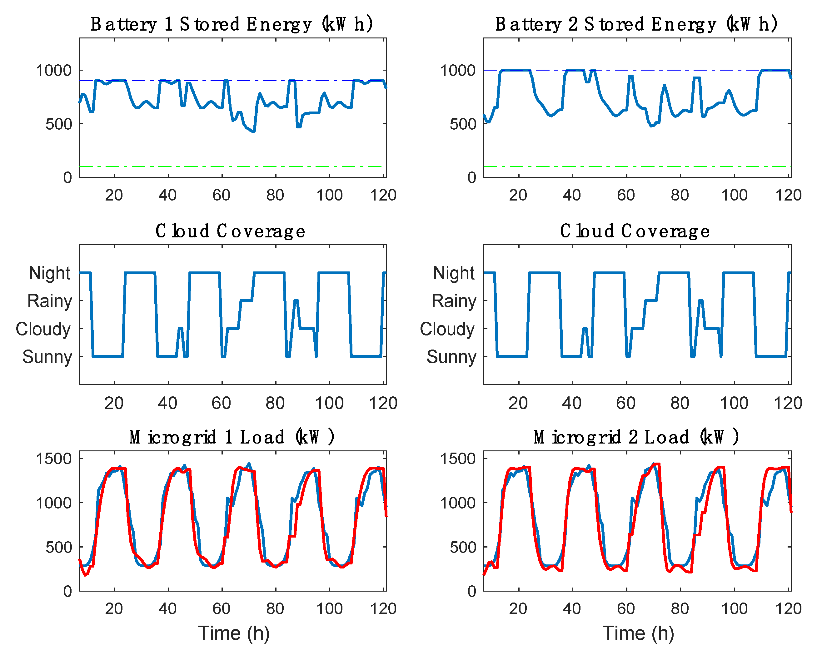
Figure 7 shows simulation results that cover a period of 5 business days. Since commercial load behavior is more predictable due to its nature, we were able to use the load profile as a collection of setpoints, and not as an input or as a disturbance. In that respect, our approach differs from most other methods described in the literature. We should also note in this context that due to low or zero inertia related to batteries and solar energy, any small imbalance between the supply and demand can be handled by the batteries and PV arrays.

Another distinguishing feature of the proposed control strategy is that it does not rely on weather forecasts or load forecasts—instead, it considers cloud coverage, the hour of the day (or night) and battery energy setpoint in each mode, and uses this information to compute the required control action. The choice of setpoints is dependent on cloud coverage, since on sunny days we want the battery fully charged, and on rainy days (or at night) we want to allow the battery to discharge as much as possible. In fact, once r(t) jumps from i to j, the optimal control action is to switch from K_i to K_j. The only requirement is that the information be available when needed (this is not difficult to do with existing computing technology).

The two batteries are chosen to have different storage capacity, and their energy output represents the control action. The storage capacity for batteries 1 and 2 is 1000 kWh and 1100 kWh, respectively. We assumed, however, that the SoC for both batteries lies between 10% and 90%, (these limits are shown by dashed line in Figure 7 top graph). The existence of such limits prevents deep charging/discharging, which can adversely affect the life span of the battery.

Our simulation results show that on sunny days both batteries are charged to their maximum level using solar energy and energy provided by the utility grid. During the night, they discharge to satisfy the demand. Figure 7 also indicates that batteries cannot fully charge during cloudy or rainy intervals (and during the night they may discharge below 50% of their capacity). It is important to recognize, however, that neither battery discharges completely, since both μGrids are connected to the utility grid.

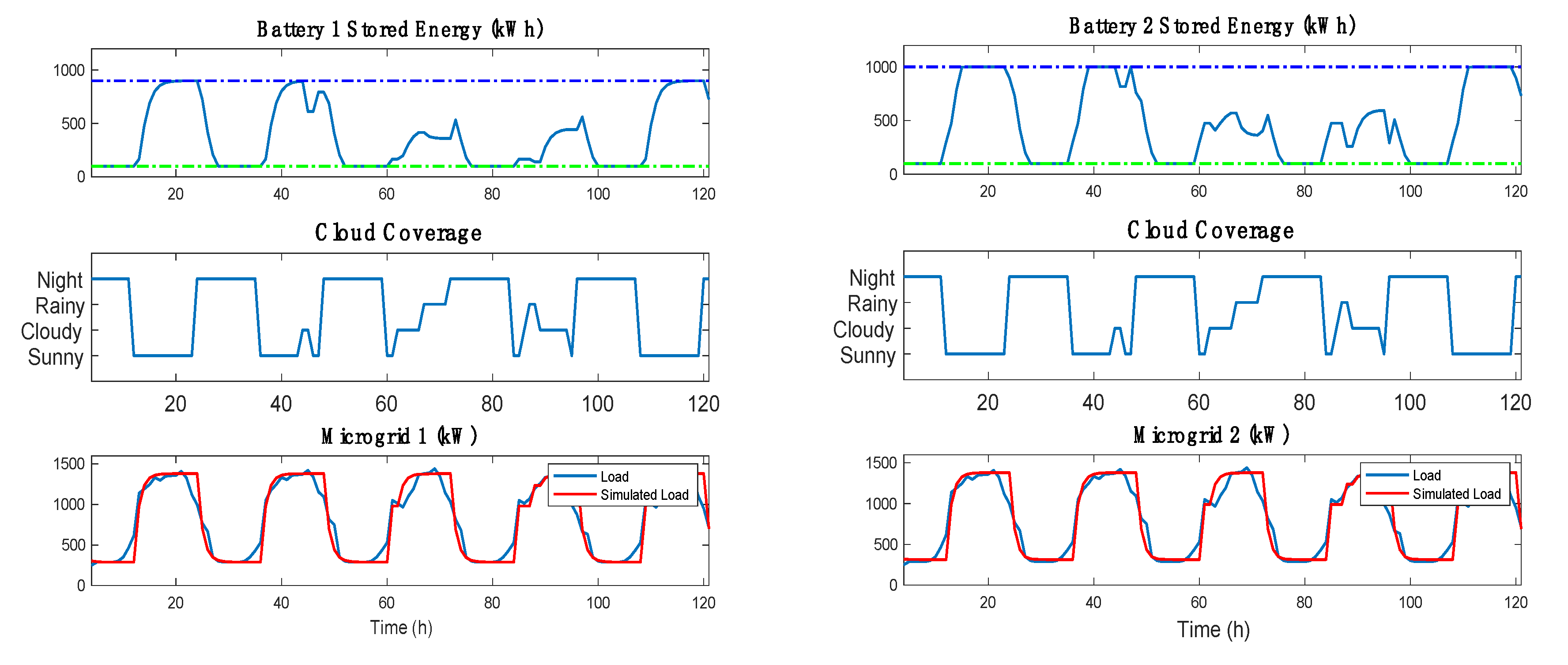
Figure 8 shows how the system behaves when the μGrids operate in the islanded mode. It is readily observed that in this case the battery must discharge completely in order to satisfy the demand, although the load demand during the night is only about 1/3 of the energy required for the day. We should also note that on a sunny day the battery will be fully charged (which is similar to the connected mode), but on partly cloudy or overcast days it discharges more than in the connected mode. Unless the effects these large daily swings are mitigated in some way, they can reduce the battery’s life span, and perhaps even damage it. This is obviously undesirable, and needs to be addressed. In our future work, we plan to do so by adding controlled secondary generation.

To properly evaluate the simulation results presented in this section, it is important to keep in mind that they were based on three novel ideas. First, a simple continuous multivariate dynamic model was obtained which permits the use of an optimal stochastic control strategy. What is particularly appealing about this approach is the fact that the model does not have to be exact, and that the obtained analytical control law guarantees optimal use of solar energy and battery storage. Second, we use the fact that commercial loads are predictable and can afford to become self-sustainable, because the cost of outages outweighs the cost of solar panels and storage. The fact that loads are grouped by μGrids, allows for a more uniform load distribution. Finally, we should point out that the proposed control design does not rely on weather prediction, since the JLQC method allows us to obtain appropriate control actions using offline weather data. A Monte Carlo method is used to generate a set of possible scenarios of cloud coverage using the obtained transition probability matrix.

When comparing the results obtained using the proposed control strategy with other existing methods (such as stochastic model predictive control, multi-agent systems distributed control, and the various stochastic optimization techniques mentioned in the Introductory section), it should be recognized that this approach does not require online optimization, nor does it rely on day ahead scheduling using load or weather forecast. Furthermore, the control actions are not obtained iteratively, so there are no convergence issues. These features constitute key advantages, since they eliminate the need for intensive computation and online prediction. Because of that, the proposed control strategy is both robust and economical. There is broad consensus in the literature that this is desirable, and that offline controller design is preferred whenever possible (see e.g., [44]).

5. Conclusions and Future Work

In this paper, we proposed a simple stochastic hybrid dynamic model for μGrids that can connect and disconnect from the utility grid. This mathematical framework was subsequently used to design an optimal stochastic control strategy, whose main objective was to maintain the stability of the grid by optimizing storage and solar energy usage. The obtained gain matrix is piecewise constant, and can be calculated offline by applying the stochastic maximum principle.

It is important to recognize in this context that the resulting closed-loop system is potentially capable of self-healing when a fault occurs, or when a natural disaster impacts the grid. To the best of our knowledge, no similar model exists in the literature. Our future work in this area will focus on increasing the number of μGrids and removing the assumption that they must be physically close to each other. We will also consider the effects of adding controlled secondary generation to the subsystems, and examine how the system dynamics change when the μGrids are connected.

A potential limitation of the proposed control strategy is that it does not explicitly incorporate constraints on battery storage capacity. To ensure that these constraints are met, we used weighting matrix Q and R (as well as the setpoints on battery storage capacity) as tuning parameters. Our simulations established that this approach is effective, and that the resulting control law can accommodate discontinuities (jumps) which are due to sudden changes in solar generation, battery capacity, and load demand.

We should also note that the approach described in this paper implicitly assumes that the 24-h load demand follows a predictable pattern. When that is not the case, the gain matrix becomes time dependent, and the control design becomes considerably more complex (in part because of convergence issues related to the Riccati equations). We plan to investigate this problem in our future research.