Abstract
This paper is devoted to investigating the effects of high-speed elongation of arcs inside ultra-fast switches (ucontact 5–80 m/s), through a 2-D time-dependent model, in Cartesian coordinates. Two air arcs in series, one between a stationary anode and a moving cathode and the other between a stationary cathode and a moving anode in the arc chamber, are considered. A variable speed experimental setup through a Thomson drive actuator is designed to support this study. A computational fluid dynamics (CFD) equations system is solved for fluid velocity, pressure, temperature, and electric potential, as well as the magnetic vector potential. Electron emission mechanisms on the contact surface and induced current density due to magnetic field changes are also considered to describe the arc root formation, arc bending, lengthening, and calculating the arc current density, as well as the contact temperatures, in a better way. Data processing techniques are utilized to derive instantaneous core shape and profiles of the arc to investigate thermo-electrical characteristics during the elongation progress. The results are compared with another experimentally verified magnetohydrodynamics model of a fixed-length, free-burning arc in the air. The simulation and experimental results confirm each other.
1. Introduction
Studies show that about 20% of industries have to change 5% to 10% of their circuit breakers (CBs) by 2020, due to the increase of the short circuit level [1]. Techno-commercial studies prove the feasibility of fault current limiters (FCL) and many investigations have been initiated and reported by EPRI and CIGRE [2] to design a practical FCL. Hybrid FCLs are among the most powerful current limiters developed so far and the most affordable idea in terms of cost [3]. In one of the hybrid FCL designs, a simple multi-contact fast switch (FS), along with the inherent features of the series arcs, has been used to commutate the current to current-limiting parallel branches [3]. Mechanical FSs can also be used in HVDC interrupters [4,5,6] where a rapid operation is required and semi-conductor switches are not preferred due to their high cost-loss, harmonic effects, sophisticated control, and continuous maintenance. Electromagnetic driven switches make 100-µs close/open times possible, which, in comparison with semiconductor power devices, are low-loss in ON-state and more reliable.
The actuating mechanism of many fast switch designs is based on electromagnetic repulsion. The theory of such a mechanism is thoroughly presented in [7] and the first patent filed in the late 60 s. Some more recent works on the design of such operating mechanisms have been reported elsewhere [8,9,10]. In a recent study, a design has been introduced to cut off 2 kA at 12 kV single-phase voltage [3,11,12], where only the mechanical model and the mechanism of FS were considered. The electrical simulations for modeling the drive and study of the effects of different parameters on the contact speed, , shows these FSs can reach 70 m/s through the optimum design [13], and then the arc characteristics will be severely affected by this fast elongation.
Because of the difficulties in the simulation of a fast elongating arc (FEA) in subsonic regimes, there is only a limited number of relevant papers in the literature. Some other researches were conducted on electrical simulations for modeling the drive, studying the effect of different parameters on [14,15,16], and application of this drive for AC circuit breakers [17], in combination with vacuum CBs [18,19] or HVDC interrupters [4,10,20]. The latter has resulted in a patent registered by ABB [21]. None of these studies investigated the characteristics of FEA in FS.
Just in [22], the first 2 ms of FEA has been modeled using a black-box approach for a very limited range of arc currents and elongation speeds, without paying attention to the arc physics. Therefore, this model is only applicable to the specific geometry within a limited range of speeds and currents. It is, also, vulnerable to the problems arising in attempts to represent electric arc dynamic processes accurately utilizing ordinary mathematical models [23]. Another reason for the study of FEA is that of replacing the greenhouse SF6 gas, where almost all environmentally friendly alternatives shall be used at pressures higher than what SF6 was utilized at. At higher pressures, the thermal conductivity is reduced at the arc quenching temperature range, i.e., below 4–5k K, which is vital for the current interruption, and so the input energy to the arc could be reduced through the fast opening method.
The model consists of the magnetohydrodynamics (MHD), the moving mesh, and the net emission coefficient (NEC), which is the difference between the radiated and absorbed power, considering the contact effect with a circumstantial treatment of heat transfer in solid parts, including the contacts. The as the output of another electromechanical finite element model (FEM) is simulated and imported into this model. Details of the electromechanical FEM model of the Thomson coil circuit, as well as technical methods for electro-mechanical measurement of fast elongated arc parameters, including the measurement noise, shift noise, and the practical way to consider their effects in simulations and experimental setup including FS geometry, are available in [24]. The first motivation of this study is to understand the physical mechanisms of arcs elongated inside the fast switches before the current zero (CZ).
A mathematical model is presented for variable-length AC arcs in contactors with elongating speeds of about 1 m/s, where the arc voltage is described by a series arc concept [25]. It is only applicable to cylindrical arcs when the temperature distribution is radial homogenous. Another already presented mathematical model for variable-length arcs tries to relate the arc voltage with the arc volume, but it is only applicable to the welding arcs when the length is changing vertically with rather low speeds [26]. All of these purely mathematical models are either modified versions of the Cassie-Mayr model and rely on energy balance inside the arc, or a modified Ayrton model for DC static arcs [27], or even a static model of welding arcs without diagonal cooling [28]. The relation between the arc length and its voltage and current has been essential, however, in other fields like arc welding, where a robust method is proposed to measure the arc length in [29]. Also, a technique to find the arc current and voltage from arc length in welding has been patented [30]. This fact can express the importance of presenting a reliable model for fast elongating arcs to solve the most critical issue related to the current commutation in hybrid FCLs/HVDC circuit breakers.
Although there are plenty of studies on the current interruption in high-voltage (HV) gas circuit breakers [31,32,33], vacuum interrupters [34], and medium voltage load breakers [35,36,37], only a few reviews on the low-speed load break switches, mostly relying on experimental findings without MHD simulations [38,39], are available. Just a few studies deal with simulations for VCB [40] and air breakers at a contact speed of about 2.5 m/s [33], which will result in a short gap before the CZ. This is the second reason for this study. In [41], the gap memory effect concerning the interrupted current is illustrated, which is more pronounced at longer contact gaps, similar to what we have here in FS.
2. Model Description
2.1. Model Assumptions
Though lots of the published investigations on MHD simulations for arcs in low-voltage miniature circuit breakers (MCB) and medium or HV SF6-CBs are mentioned, there is almost no investigation on MHD simulation of FEAs because of some issues and simulation difficulties [42].
Increasing the fluid velocity, U, increases the ratio of advection to thermal diffusion (Peclet number). For the heat equation, this condition necessitates the use of numerical stabilization and a finer mesh. Reaching convergence on simultaneous solving of heat transfer and laminar flow (LF) equations, especially at high velocities and for gases with low viscosity, is a big challenge, as these two physical concepts are acting against each other. Sometimes, time step reduction can help, but it becomes more complicated if the generated heat increases by increasing the arc current.
Tiny meshes in the presence of a moving part result in distorted mesh elements in a few intervals. To overcome the mentioned issues and trade-off the accuracy, time, and complexity, 2-D arc simulations are used. When there are no strong vortices inside the flow, 2-D simulations are accurate enough [43]. This assumption has some effects on the gas flow that will be discussed later. In local thermodynamic equilibrium (LTE), which implies local chemical as well as thermal equilibrium [44], the plasma can be considered as a conductive fluid mixture and, thus, be modeled using the single-flow MHD equations instead of two separate flows of electron and ions. The very thin-state plasma flow can be modeled as laminar and the effects of symmetry assumption on asymmetric turbulent flows (TF) are ignored due to smaller length scales in Reynolds number (Re).
2.2. Experiment Setup and the Numerical Geometry
Figure 1a shows the elements of the prototype FS. The electromagnetic actuator of CB used in this study consists of a spiral coil in multi-layer formation, which is connected to an L-C current source through a fast-closing switch. The energy storage device consists of a capacitor bank and is connected to the current discharging coil.
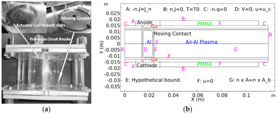
Figure 1.
(a) Elements of prototype fast switch (FS) and Thomson coil, (b) 2-D geometry, and initial conditions.
Moving contact (MC) is made from aluminum (Al), while the fixed contacts are made of copper (Cu). The initial gap between the electrodes is 2 mm. The wall of the chamber is made of transparent Poly-methyl-methacrylate (PMMA), known as plexiglass. The length of the arc chamber is 11 cm, and there are two pairs of open hatches at the bottom and the top of the chamber, as shown in Figure 1a. The moving contact is accelerated by the repulsive force generated by a Thomson drive. An appropriate two-dimensional geometry of FS, including the initial conditions, is shown in Figure 1b. The gravity acts in the negative direction of the X-axis. The sharpened edges of the contacts are bent. Avoiding sharp edges is essential in solving the flow and the heat transfer equations because the sharp points generate a very high current density in terms of numerical resolution, which results in very high-temperature spots, leading to an unrealistic heat and fluid flow. The gaps between fixed and moving contact and areas around contacts are the points with intense changes in the mesh shape, as well as in the value of the heat and fluid variables. Therefore, these areas are modified by two parallel lines, and rectangular boundaries are defined around the fixed and moving contacts as hypothetical boundaries, as shown in Figure 1b. These hypothetical boundaries allow for a smaller mesh in these areas, and secondly, help to solve the moving mesh by path definition. To calculate the arc parameters in the FS model, predefined variables must be calculated in the specific regions of each arc. Therefore, another hypothetical axial boundary is defined in the center of the model (y = 0), as shown in Figure 1b, which outlines the scope of the definition of variables for two series arcs in FS. Studies have shown that 2-D axisymmetric cannot be applied, even with significant simplifications because of two reasons:
- First, the two arcs formed in FS are not symmetric. In addition to the random phenomena and the incommensurability of the two arcs in series inside the CB, the location of the anode and the cathode is opposite in two arcs, so two series arcs are entirely asymmetrical.
- Even if two arcs were symmetric, the object is not symmetric. So, the obtained solution of the axisymmetric model cannot help to determine the shape and length of arcs. Therefore, the model must be defined in Cartesian mode (2-D).
2.3. Properties of the Material
2.3.1. Gas (Air-Al Plasma)
Thermal plasma properties of air-Aluminium vapor mixtures in [45] show that even a small amount of metal vapor at atmospheric pressure has an appreciable influence on the radiation and the electric conductivity (σ), but a negligible effect on the other features. The effect of metal vapors on σ is dominant in low-current arcs while the impact on radiation dominates at high currents [46] due to higher temperatures (T).
Plasma conductivity in the presence of 1–3% metal vapor in 11,000–13,000 K, is about 20–30% higher than of a pure air plasma [47,48], which is modeled here. When the current is lower than 1 kA, metal vapor resides only in two small regions (1–3 mm) in front of the two electrodes because of limited electrode vaporization [46,49]. Consequently, the arc temperature drops significantly in these small regions near the cathode [50,51]. Then, arc voltage (Varc) in low current mode will not be sensitive to the presence of metal vapor [49,51].
If absorption is ignored (thin layer) then metal vapor increases the NEC, but if absorption is considered then the presence of Al vapor despite Cu reduces the NEC in the temperature range of 10–15k K, if the Al mixture ratio is less than 5% [45] and arc radius is less than 5 mm, which applies to our study. The NEC decreases by an increase in the arc radius [52]. The reported results are utilized to obtain the thermodynamic properties of hot air, including heat capacity, viscosity, density, thermal and electrical conductivity, as well as NEC for the temperature range up to 25,000 K at constant atmospheric pressure [53,54] and is calculated for higher pressure (20 bar). Although the exact formulation of the energy transport by radiation is very complicated, the three mostly used methods are P1, method of partial characteristics, and NEC.
A comparison between these methods is discussed in [55]. The NEC has acceptable accuracy and less entanglement in the range of the optical thicknesses and arc temperatures, (10–15k K and 2–6 mm) [56]. The Air-Al mixture and NEC absorption effect in the presented model will be explained here.
The core diameter varies along with its length at different times. This variation is shown in Figure 2a.
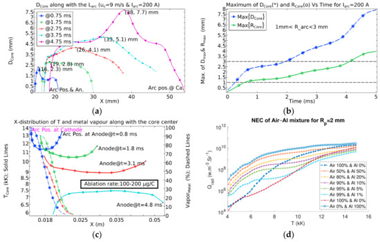
Figure 2.
(a) Variable core diameter along with its length, (b) Maximum of core radius, (c) Distribution of T and metal vapor along the core center, and (d) net emission coefficient NECair-Al in arc chamber for 200 Apeak.
As it is shown in Figure 2b, the maximum radius of the core varies between 1 mm and 3 mm. So, the radiation absorption radius, Rp, for the NEC model is assumed 2 mm. The ablated mass for Cu electrode in low currents is calculated around 100–300 µg/C [57] and in our stationary study was around 316 µg/C [51]. Although the melting point of Al is half of Cu, its latent heat of evaporation is twice the Cu. Assuming a similar ablation rate will result in 150–300 × 10−3 cm3 Al vapor. By utilizing the particle tracing method [51], the ratio of Air-Al is calculated and it is shown along with the core center in Figure 2c, which complies with other studies [49]. According to [58], the influence of changing the arc radius from 1 mm to 10 mm on NEC for air plasma in the temperature range of 7–15k K is not significant, and its gradient by increasing the arc radius is negative. So, finding an average radius for the arc gives an accurate estimation of NEC. But according to [45], the influence of metal vapor percentage is enormous at this temperature range. So, metal vapor has been considered, and the arc radius was averaged. Based on the reported NEC of air-aluminium mixture [45] and temperature distribution in Figure 2c, NEC in the arc chamber is calculated through recursive studies to minimize the relative error.
The result is shown in Figure 2d. The volumetric proportion of Al-vapour in a 2-mm gap between electrodes is more than 90% at the start of the arc. Particles have Maxwellian speed distribution, and contact is moving, which results in FEA. So, particles disperse along the arc length, and the mixture ratio decreases as time elapses. Most of the Cu particles remain near the fixed cathode while Al particles are dispersed by moving cathode displacement, as velocity inside the core is around 50 m/s at 0.5 ms but falls to 5 m/s at 1.5 ms. So, the mixture ratio of Al falls to below 5% in an arc core.
The main parameters of the utilized model are the transport and thermodynamic properties of gas mixtures, which would be obtained from the articles or could be calculated through chemical physics [59,60] for pressures and mixtures other than what is reported in the articles. Software packages handle these chemical physics calculations. Here, we used the PLASIMO® package [61], and the electrical conductivity, total heat conductivity, mass density, NEC, viscosity, and heat capacity of pure air and air-Al mixture at 1 and 20 bar at different mixture ratios and pressures are presented in Figure 3. The legends for all sub-figures are the same as Figure 3a.
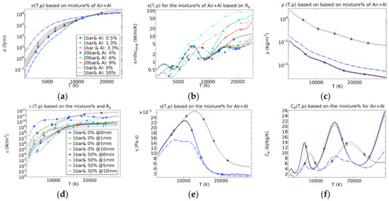
Figure 3.
(a) Electrical conductivity, (b) Heat conductivity, (c) Mass density, (d) NEC, (e) Viscosity, and (f) Heat capacity of pure air and air-Al mixture at 1 and 20 bar at different mixture ratios.
The changes in the pressure are very small in this study so its effect on vaporizing temperature is ignorable, but it could be considered as it was explained in the above through assuming a two-phase thermodynamic system and utilizing the method explained in [62].
2.3.2. Solids
The necessary parameters for the solid parts, including Al [63] and Cu contacts, as well as PMMA [64,65,66] enclosure to be considered in the numerical model, are presented in Table 1.

Table 1.
Required parameters for modeling of solid parts.
2.4. Equations, Initial, and Boundary Conditions
2.4.1. MHD Equations and Sheath Model
In general, the MHD method is time-consuming but with less data acquisition costs, while many rapid mathematical models do not care about the data acquisition costs. So, some rapid models are full of coefficients, the application of which is inevitably condemned to death after an ad hoc implementation. Therefore, it is essential to define a model description as much as possible on the data flow and information, which is the case of the MHD simulation where a mathematical model that stands on such a solid basis will have a high probability of being applied, and so tested and improved, in a continuous way [67]. That is the reason for the vast utilization of the MHD tools for the design and performance evaluation of switchgear [68]. Four groups of equations used in this study are the current conservation equations Ampere’s law and Lorentz force, HT, and Navier-Stokes equations (NSEs) for an incompressible fluid, including conservation of momentum and mass. Details of equations were already presented for the fixed contact simulation [51]. In Newtonian fluids (all gases and most non-viscous liquids [69]), if the Mach number (Ma) is more than 0.3 or the T inside the fluid changes significantly and rapidly, the fluid is considered compressible. In our study, although the T rises sharply, the changes are not in a vast range, and calculation shows that Ma is not more than 0.3. Also, the Re is relatively small, so the flow is laminar in each layer [51]. The T in the core is in the range of 9–15k K and densities of ions and electrons at this temperature are high enough to consider that NSEs are valid for highly ionized air plasma [51]. This assumption is justified by the high plasma pressure and the large estimated electron densities in the order of 1018 cm−3 [44]. Here, the sinusoidal 50 Hz 200 A current source is applied to the terminals, as shown in Figure 1b.
The initial conditions for these equations are zero potential at moving contact and zero current density at the outer wall of ACH, as shown in Figure 1b. Due to the current injection direction in the quarter-cycle simulation, the lower side of the moving contact and the upper fixed contact act as an anode, while the lower fixed contact and the upper side of the moving contact are the cathodes. The required parameters to model the effect of the Al and Cu cathode and anode are obtained from [66,70]. To solve the heat transfer equations together with the magnetic field equations in a 2-D domain, the thickness should be considered, which is added as dz = 10 mm compared with 2-D axisymmetric equations based on arc diameter.
As it is shown in Figure 1b, the top and bottom of the enclosure, interior arc chamber, as well as the outer surface of the walls are modeled with the ambient temperature T0, which meets the actual status. It is also assumed that heat transfer from the open points to the outside is negligible. Therefore, these hatches are modeled as thermally insulated surfaces (.
As the time steps and solution methods to solve the MHD and electrodynamic drive are different [71], an appropriate approach is an asynchronous solution. Measurements, and electrodynamic drive simulations, show that moving contact reaches a constant speed at the start of the arc [24]. So, the simulated speed from the electromechanical solution is imported into the fluid flow model as . The influence of thermionic electron emission (3–7) is not significant on the current density (J), as at the highest melting point of Cu cathode 4.16 × 10⁻⁵ at T = 1356 K, while J at the cathode is in the order of 9.3 × 10⁸ . Increasing T does not ensure observable electron emission since Cu will melt and then evaporates or decomposes, but it affects the contact temperature by keeping the continuity in heat transfer equations. Although the first studies on liquid metals [72] show an explosive electron emission from liquid cathodes in special conditions and for a limited time, as far as we know thermionic emission data exist only for polycrystalline solid-state copper emitters [73] and Cu is not the ideal thermionic emitter due to its relatively low melting point (1356 K), which limits the working temperature region to 800–1100 K or so [74]. The cathode temperature does not reach the melting point in the first cycle, so thermionic emission from melted Cu is ignored.
The required parameters of Cu contacts are = 4.94 V, and = 120.2 [66,70]. According to (6), the cathode temperature change is the result of the energy absorption and electron emission from the cathode, i.e., overcoming the space charge energy level, and the potential of the plasma ionization layer of positive ions ( = 15.5 V) near cathode regions [75].
According to (7) at the anode surface, the temperature change in the anode is a result of the absorption of electrons at the anode, i.e., overwhelming the energy level because of the accumulation of electrons near the anode.
and
are voltage drops (Vd) as a function of J over the fluid–contact interface without taking any physical aspect of the sheath into account [76].
2.4.2. Moving Mesh and Mesh Validating
As already noted, another simulation difficulty is fast movement. To consider the mechanical motion, Plexiglas walls and fixed contacts are modeled with fixed mesh, but the rest of the interior of FS is defined as a region with free deformation, and a mathematical lema named moving mesh [77] is used to model contact motion. The mesh around the contact moves with . The maximum and minimum sizes of mesh elements were selected as 1.06 mm and 15.2 µm, respectively, but as it is shown in Figure 4b, boundary layers of fixed contacts, as well as the edges of the fixed and moving contacts, are modeled by a fine mesh with a minimum/maximum size of 0.76/70 µm suitable for CFD.
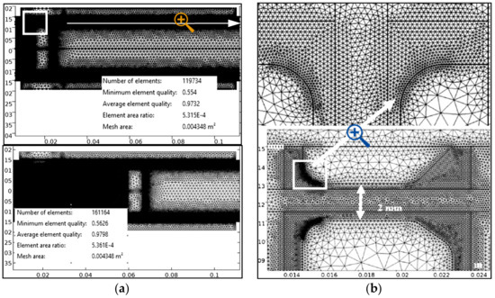
Figure 4.
(a) Moving mesh with 119,734 elements in 43.48 cm2 at first and 161,164 elements at the end and (b) Extremely fine mesh defined around contacts and gap.
The areas between the sidewalls and the bottom of FS, as well as the linear boundaries parallel to the walls, are modeled by a fine triangular mesh with a maximum size of 150 µm.
To perform a more realistic fluid flow simulation next to the walls, a boundary layer mesh on all internal walls is defined. The final mesh has around 120,000 elements, as shown in Figure 4a. The mesh element quality is shown in Figure 4a is a dimensionless quantity between zero and one, which is an important aspect when validating a model. This measure is based on the equiangular skew. It penalizes elements with large or small angles as compared to the angles in an ideal element. Poor quality elements are considered for quality below 0.1 [78]. Contact movement causes the meshes to be squeezed and drawn, resulting in element quality reduction. Massive compression and stretch cause the model to be unstable and unsolvable. If the mesh overlapping reaches a predefined level, the solution is stopped, and the mesh is repeated considering the previous solution as the initial condition for the new meshed geometry.
In this way, an automatic mesh is generated almost every 120 µs up to 44 times in the course of the simulation, so that the output of mesh number 45 according to Figure 4a contains about 161,000 elements in 43 cm2 with the same quality as the first mesh. High mesh density below and around moving contact, as well as next to the walls, is visible. Taking into account the equations modeled with this number of mesh elements leads to 460,000 degrees of freedom (DoF) in equations for the primary mesh, which finally reaches more than 635,000 DoF by increasing the number of meshes. The minimum mesh quality that has been ensured for each of the models that have been solved is 0.55, with an element area ratio of about 5.3 × 10⁻⁴. In general, the triangular mesh is a quick and straightforward way to obtain meshes of high element quality but comes with a diffusion cost. However, the extra diffusion can sometimes be desired, since it becomes easier to achieve convergence. A precisely defined triangular mesh specifying the distribution of mesh elements along an edge, in addition to Refinement of the Corner to decrease the element size at sharp corners, is perfect for our model, where the mesh serves as a starting mesh for mesh adaption. The obtained solution is then used to refine the mesh based on some indicator function. Finally, the adapted mesh is used to simulate the time interval again. After examining different methods, the parallel sparse direct and multi-recursive iterative linear solver (PARDISO) [79], as a stable time resolution method, was used while the Jacobian matrix was updated at each step. Absolute tolerance of 5 × 10⁻⁴ and at least 1 ps time steps at the start of the solution and maximum 2 µs is vital for modeling of Varc in the last 20 µs of the arc cycle accurately.
2.5. Arc Ignition
To initiate the arc in the most of the other researches, a predefined conducting column, usually rectangular with a temperature between 7000 and 10,000 K, is assumed between two contacts, which has the role of a thin melting wire in practical experiments [71,76,80], but it causes the shape of the arc and its movement to be unrealistic during the initial arcing period. As an accurate arc shape and therefore Varc in the first 200 µs is necessary for current commutation purposes, a different approach has been taken here. The initial air conductivity is assumed to be 1 s/m wherever its conductivity is less than 1 s/m. By taking this approach along with electron emission from contacts, the arc starts from the sharp points and with an accurate initial shape. Then, the arc region can be determined using the σ distribution.
2.6. Turbulent vs. Laminar
2.6.1. Plasma Numbers
Critical Re must be determined through experiments or numerical simulations for each configuration.
The maximum of Ma, Peclet number (Pe), Re, and Prandtl number (Pr), calculated in each cell of meshes for the whole of simulation time in an arc of 200 A, are shown in Figure 5. Ma is much less than 0.3. Pe, the product of the Re and Pr, is very large. The studied case is, however, similar to the flow inside a cylinder, where for 41 ≤ Re ≤ 103 an unsteady but predictable LF with counter-rotating vortices shed periodically from the cylinder is observed [81]. If Re > 103, vortices will be unstable, resulting in a turbulent wake behind the cylinder that is ‘unpredictable’ [81]. There is a transition to an entirely TF. As the stream begins to transfer to the turbulence regime, fluctuations appear in the flow, even though the inlet flow rate does not change with time. Then, it is no longer possible to assume time-invariant flow. So, it is compulsory to solve the time-dependent Navier-Stokes (TDNS) equations.
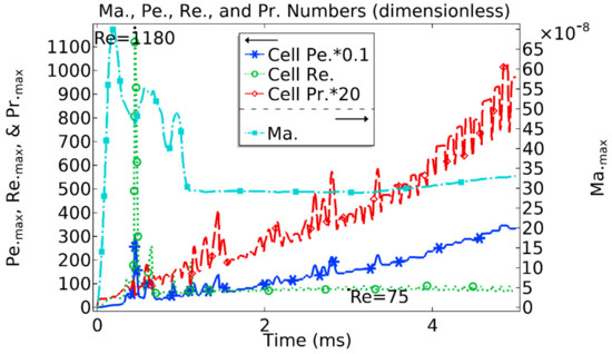
Figure 5.
Maximum of cell Peclet number (Pe), Mach number (Ma), cell Reynolds number (Re), and cell Prandtl number (Pr) for the whole of simulation in 200 Apeak arc.
2.6.2. Turbulent Model
From Figure 5, Re becomes more significant than 103 at 0.5ms. This is an indication of TF. So, the algebraic Y-plus TF model is used in the first 500 µs of the simulations. Figure 6 shows the arc temperature distributions at different times. The application of the TF model results in lower temperatures and a different shape for arc between contacts (Figure 6d).
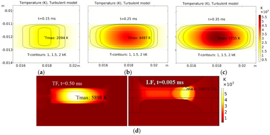
Figure 6.
Arc temperature surface modeled in turbulent flows (TF) at (a) 0.15 ms, (b) 0.25 ms, (c) 0.35 ms, and (d) Comparison of arc shape in the laminar and TF model for an arc of 200 Apeak.
No large vortices field occurs inside the arc due to a border between the thermal plasma column and TF around it [82]. So, if the mesh is fine enough to resolve the size of the smallest eddies in the flow, the laminar model will remain suitable to reduce the time costs.
2.7. The Arc Roots and the Sheath Model
The simulated temperature distribution in the arc core and the contacts at two different times, 250 µs and 1 ms, are shown in Figure 7a to identify the dominant physical processes inside the arc during different phases of arcing. Up to 250 µs, the arc is sliding in the opposite direction of the moving contact (MC) displacement due to the cold air blowing at the arc column, (see Figure 7c). As it is shown in Figure 7a, in the first 250 µs, the arc length is constant, and the temperature distribution is almost homogenous inside the core, except for the anode and cathode regions. Therefore, the arc-elongating speed is zero before 250 µs.
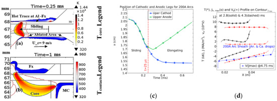
Figure 7.
A Core and contacts’ temperatures show (a) Arc sliding along the contacts up to 0.25 ms, (b) Arc elongating between fixed (Fx) and Moving (MC) contacts at the speed of 9 m/s, (c) X-position of arc roots vs. time, and (d) Temperature, current density, and voltage profile along the contour of Jmax.
The arc is not in LTE in these two regions, and the NSE condition is not fulfilled. But simulated results are not so far from the measurements [24]. As it is shown in Figure 7a, arc sliding causes a hot trace at the contacts, which have a temperature range of 600–900 K based on Tcontact legend. As it is shown in Figure 7a, the arc temperature is higher than 10k K, i.e., the air is highly ionized, and the NSE assumption is valid. From 1 ms, as it is shown in Figure 7b, the arc is elongating between two points at the contacts. The arc root model is based on [76,83] and the temperature, current density, and voltage profile along the contour of Jmax in Figure 7d show the effect of this model.
3. Results
3.1. Temperature and Conductivity Dynamics
Figure 8a,b shows σ contours and the point of the maximum conductivity at 1.35, 2, 2.75, 3.45, and 5 ms in an arc of 200 A. The bright-dark part (green contour) is named core of arc. The rest of the arc inside the red contour is named arc column. The arc light is due to radiation that is proportional to T4. So, the arc column boundary is defined as σ = 1, which is equal to 3300 K but the core is the gliding section of arc (σ > 600, which is similar to 6700 K in air temperature) which is passing more than 80% of the arc current.
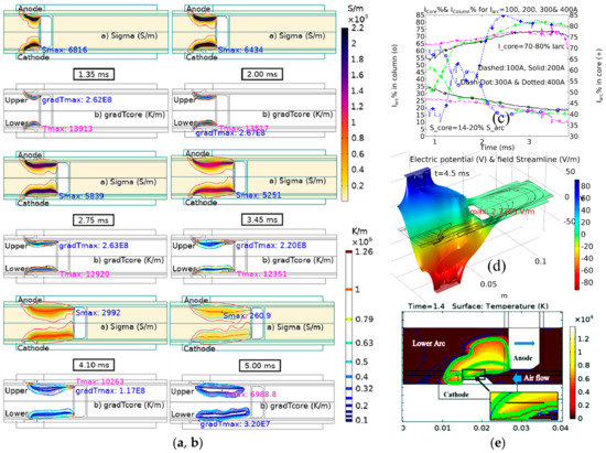
Figure 8.
(a) σ contours and the point of maximum σ, (b) Contours of T-gradient at 1.35, 2, 2.75, 3.45, and 5 ms in an arc of 200 Apeak, (c) Percentage of Iarc = Isource divided between core/column, (d) Electric potential and electric field at 4.5 ms showing anodic and cathodic Vd, and (e) Zero gradient contours for Jnorm (green), σ (red) and T (blue) at 1.4 ms on the T-surface.
Figure 8 shows contours of (a) σ, and (b) the temperature gradient at 1.35, 2, 2.75, 3.45, and 5 ms in an arc of 200 A. It shows that before 2.8 ms the temperature gradient inside the core is high, but after this time it becomes more uniform inside the core center. The point of maximum temperature (Tmax) and maximum conductivity is clear in the figures. It is a point with the same color as the related text at the upper left of it. It is close to the moving anode and then shifts to moving cathode but before the CZ falls to the core midpoint. Figure 8d shows that after 2 ms of arc ignition and independent of arc current magnitude, the core is passing 70–80%, and the column is passing around 20–30% of current. The axial centerline of J in core shown by the red line is where the J gradient perpendicular to the arc column is zero. It is not the spatial centerline, so the core shape and thickness on both sides of the arc center line are not similar due to massive gas flow to the outer sides. Figure 8e shows zero gradient contours for the normal component of current density Jnorm (green), σ (red), and temperature (blue) at 1.4 ms. Due to the relatively linear relationship between temperature, σ, and current density in the range of 10–14k K, these contours overlap.
3.2. Simulated vs. Captured Appearance
Figure 9a displays time-tagged pictures from simulated results of the arc border (outer contour) and core border (inner contour) based on the above definition, including the point of Tmax in 200 Apeak arc (upper left of Tmax). Figure 9b illustrates the arc imaging in FS taken by a 15,000 fps recorder. A dark green filter is used at the camera to prevent saturation, so pictures before 1.57 ms and after 3.37 ms are not so visible. The visual appearance of the curved and the other pulled simulated cores and the core brightness at 2.8 ms (before the change in mode) are confirmed by the experimental results in Figure 10b. Arc current is calculated from:
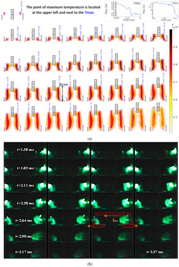
Figure 9.
(a) Time-tagged simulated results of arc and core boundaries for two arcs in series, point of Tmax in 200 Apeak arc, and (b) High-speed imaging with 15,000 fps.
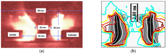
Figure 10.
(a) Enlarged image of the arc and (b) Its light intensity contours extracted by the image processing vs. simulated arc at 2.8 ms.
A low-frequency (f ≤ 100 Hz) arc on each half-cycle mirrors a direct current arc, the contact separation initiates the arc, and when the current reverses the electrodes interchange their roles as anode or cathode [84]. Simulated and measured arcs are not at the same cycles, so electrode positions are reversed. From Figure 9a, the arc starts with a Tmax of 14,790 K on both sides of FS from the sharp points of the contacts. Then it moves downward along the contacts and stays at its bottom because of the intense flow on it. When the arc comes out of the gap between the contacts, its T decreases up to 1000 K after 0.25 ms. Then it is elongated, but before 3.6 ms, its temperature is not reduced so much despite the current falling according to Equation (3), and it remains constricted. It is observed that the core is highly compact, hot, and luminous before 2.95 ms, and the arc boundary is more spacious than the core border.
This mode is obvious from high-speed imaging with 15,000 fps in Figure 9b and we call it a constricted mode. At 3.83 ms, the T dropped sharply. The position of Tmax has been recorded near the moving contact before the mode change, but later it moves to the center of the arc at 4.25 ms. That is, the arc starts to cool on both ends, but the current is not zero yet. We refer to this as a dispersed mode.
3.3. Impact of Thermionic Emission
Thermionic emission acts as a heating source, and it is of crucial importance for contact temperature and ablation simulations, especially for the Cu cathode. The effect of modeling the electron emission from the cathode on the Tmax of contacts is compared in Figure 11. “C. Eff.” refers to the contact effect and means considering the thermionic emission in simulation. Considering thermionic emission, the temperature of the moving contract does not differ significantly, but as it is shown in Figure 11a the Tmax of the fixed cathode increases at 3.4 ms from 707 K in Figure 11b to 1103 K at 1.8 ms, while the Tmax of the fixed anode increases from 660 to 800 K. Contact erosion mostly happens near the fixed Cu cathode and then moving Al anode. It was modeled in detail and reported in other recent research [51] and it is also clear from Figure 12a.
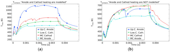
Figure 11.
Tmax of contacts (a) with thermionic emission modeling, (b) Without thermionic emission modeling in 200 Apeak arc.
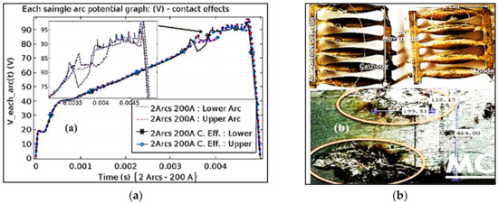
Figure 12.
(a) Ablation on fixed and moving contacts (MC in figures means moving contact) and (b) Two 200 Apeak arcs with(out) thermionic emission modeling.
Figure 12a compares the simulated voltage for two 200 A arcs with and without thermionic emission modeling. It reveals that the contact modeling in the first 3.5 ms has no significant effect on Varc for two 200 A arcs, but it affects the voltage in the last 1 ms. Anodic and cathodic Vds are modeled in both simulations. Figure 12b shows the melted/ablated points on fixed and moving contacts of the prototype switch. As predicted by the simulations, a trace of arc root is visible on the fixed cathode contact, and the most significant erosion happened at the lower part of the fixed contacts.
3.4. Arc Mode Change and Interaction of Arcs in Series
Figure 13 shows the influence of the arc mode change and its effect on increasing the core area. It shows the instantaneous area of the whole arc and its core, as well as the ratio of core-to-column area, for 100 and 200 A arcs with(out) thermionic emission modeling. The slope of the ratio increases suddenly by a factor of 2.15 for 200 A arcs between 2.95 to 3.83 ms, which is the time of change in the arc mode and means the core is not constricted any more. A single 100 A arc is simulated by applying to one of the fixed contacts. The arc area is smaller, but mode change happens in lower currents.
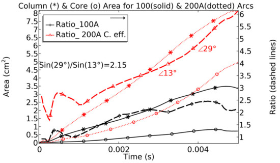
Figure 13.
The core area, and the ratio of core-to-column area, for 100 and 200 Apeak with(out) thermionic emission.
4. Discussion
4.1. Cathode and Anode Vd
Figure 14a shows arc boundaries, the σ inside the core (yellow), Electric potential (V) contours (red and blue contours perpendicular to arc and core boundaries), arrows, and contours of Jnorm in logarithmic scale (in green). The numbers in black are the V-contour tags in 2.5 V steps between. A zoomed view of conductivity for the 1 mm-thick layer near the cathode is shown at the upper right corner of Figure 14a and in Figure 14b for the upper and lower sides of the moving contact. The σmax, Tmax, and consequently Jmax are evident in this view, and numbers in magenta are the J-contour tags.
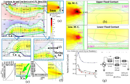
Figure 14.
(a,b) Arc boundaries, V contours, and Jnorm in Log. scale and the zoomed view of the near electrode areas at (c) Fixed cathode, (d) Moving anode, (e) Diagram of from cathode to the core gradient line, (f) Diagram of the from anode to the σmax, and (g) Simulated arc and core resistance and piecewise linear equivalent circuit of for 200 Apeak; (An, Ca, and MC in figures refer to the anode, cathode, and the moving contact).
The arc column gets narrow near the cathode, while it has a bezel shape near the anode. From Figure 14c,d, it is obvious that the arc core (yellow section) has a sharper tip near the cathode than the anode.
The zoomed view of these tips is shown in Figure 14e,f, showing the sheathes. The diagrams of the from cathode to the core centerline and from anode to the σmax are shown in this figure. The equipotential lines between the core and the cathode wall are very dense, which means a rather uniform field and significant linear Vd in the cathode sheath; this finding is shown in the conductivity curve of Figure 14e and is in line with other studies [86]. The sheath effect increases the arc resistance () in front of the electrodes, as it is recognized from the broken and deformed σ diagram of the cathode sheath in Figure 14e.
It shows a change in σ (blue) near the sheath layer and the constricted V contours (brown) near the electrodes. The J at the cathode depends on cathode material, while it is independent of the current [87]. The Jmax near the moving cathode was simulated to 3.5 × 10⁸ . The relation between J and electron temperature is presented in [75], and the sheath thickness is estimated based on electron temperature [88].
Our simulated sheath thickness is about 130 µm at the cathode, which complies with the mentioned research. At 3.75 ms, the simulation shows about 16 V drops along the 130 µm cathode sheath (123 mV/µm) and about 2–3 V drops in 55 µm (45 mV/µm) between the core boundary and anode. Simulated anodic and cathodic voltages are similar to others [89].
The thickness of electrode sheaths for arcs at atmospheric pressure is less than 0.7 mm in total. The sheath Vd and the current divided between core/column imply a piecewise linear equivalent circuit of for 200 Apeak, shown in Figure 14g with the simulated arc and core resistances.
4.2. Effects of Fast Elongation on the Arc Voltage
Figure 15a compares the measured VMeas (dash-dotted in green) with the simulated Vsimulated for 200 A, considering thermionic emission modeling. It is seen that both VMeas and Vsimulated jump from zero to 24–33 V, then step up to 40–45 V and then increase to about 75–80 V with a linear increment rate of m = 10 kV/s.
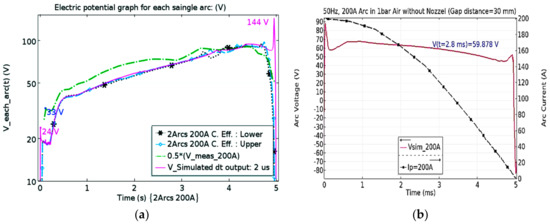
Figure 15.
Measured and simulated arc voltages for 200 Apeak arcs in (a) Prototype FS with uc = 9 m/s and (b) Fixed contact distance of 30 mm initiated by exploding wire at the same current cycle.
The shape of Varc complies with other researches [90], but the first jump of the measured voltage is higher because of higher simulated temperature in laminar modeling. The jump at the end of Varc is missed in measurement and simulation with a sampling rate of 50 µs, but it is detected with a sampling rate of 2 µs (in purple) of simulated output and is apparent in other experiments [37,91,92]. The slope of the measured and simulated voltage falls close to zero with the arc mode change. Figure 15b shows the simulated Vsim for 200 Apeak arc between a fixed contact distance of 30 mm (stationary arc) initiated by exploding wire at the same current cycle [93]. Varc is higher in the elongated state.
Figure 16a compares the measured (Dashed Line) and simulated (Solid Line) Varc for 200 A arc. The higher the , the faster the elongation and the higher the voltage for the similar arc currents. By increasing to 22.5 m/s, Varc reaches six times its value in the fixed contact distance at 200 A. Figure 16b shows the influence of elongating speed on Varc for 200 A arc. The m [kV/s] is related to the thus it increases in higher . The Varc is an essential measure for a successful commutation.
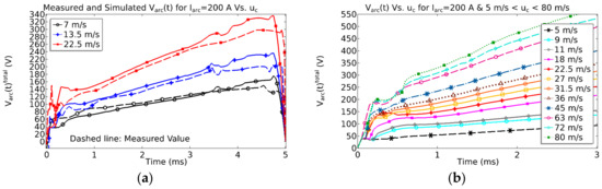
Figure 16.
(a) VMeas and Vsimulated for uc = 7, 9, 13.5, and 22.5 m/s, (b) Vsimulated in first 1.5 ms for uc = 5–80 m/s, for 200 Apeak arcs.
The failure of fast switches results in current commutation failure, and consequently failure in HVDC breakers and FCLs. The relation between the contact velocity and current is a matter of interruption performance and needs the simulation of transient recovery voltage (TRV) slopes. It is already studied through this validated model and is shown in Figure 6 of [94]. The relationship between the contact velocity and Thomson coil current or the variation in the actuator parameter was already published in [13]. Arc behavior in the failure of FS due to high currents, or insufficient through data-driven decision making (DDDM), is the target of future studies. DDDM is based on actual data rather than intuition or observation alone. The hard truth is that simulation output alone is not enough. So, making organizational decisions for failure Prediction can be utilized through different modeling techniques [95] like Gaussian Process Regression Models [96] in the failure study.
4.3. Effects of Fast Elongation on the Convective Cooling and
Figure 17a shows the maximum convection flux for 200 A arc at of 5, 7, 9, 13.5, and 27 m/s. It is also evident that convective cooling is related to . Besides, the maximum of the convection is dependent on the maximum of the U (Umax), and the Umax is dependent on the again [97]. Figure 17b shows the voltage per length for the 200A arc for of 5, 7, 9, 13.5, and 27 m/s within the first 3 ms. Dividing 50 V reported simulated voltages [98] to 8 mm distance between parallel rails [99] and it is already known that elongation increases the cooling and the Varc, total, but it decreases the arc cross-section. All these changes shall increase the resistance per unit length but, according to Figure 14g, the resistance remains almost fixed and therefore the Vd per unit length inside the arc is decreased.
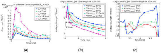
Figure 17.
(a) Max. convection flux for 200 A arc at uc = 5, 7, 9, 13.5, 27 m/s. Voltage per length of arc for (b) the first 3 ms for 200 A arcs and uc of 5, 7, 9, 13.5 and 27 m/s, and (c) the last 2 ms for 200 A arcs and uc = 5, 7, 9 m/s.
The physical reason behind this observation is that the elongation makes the arc narrower, so in a fixed length, the plasma volume is reduced, and therefore, lower energy is needed to keep the plasma in the previous condition considering fixed energy per volume for the plasma. As the current is supplied through the current source, the voltage per length is reduced. Except for the first 1 ms in the rest of this period, the voltage per length of arc remains between 2.5–4.5 V/m, which is in line with other measurements [37].
Figure 17c shows the voltage per length of the arc in the last 2 ms before CZ for 200 A arcs at of 5, 7, and 9 m/s. In this period, the voltage per length of arc remains between 1.7–2.3 V/m. The physical reason is that convective cooling is reduced, as is shown in Figure 16b. Therefore, lower input energy is needed to keep the plasma in the previous condition as the loss is reduced. Thus, the voltage per length is reduced again.
5. Conclusions
The concrete findings of this study are pinpointed here:
- Utilizing moving mesh, a detailed 2-D FEM model for an air arc plasma in a prototype FS was presented. The numerical model was established based on MHD and NEC and was validated theoretically and experimentally. Comparing with other researches and experiments, all assumptions were explained in depth.
- The presented model can be adapted to a vast range of geometries, contact opening speeds up to 80 m/s, as well as various arc currents.
- The thermodynamics and electrical behavior of FEA, as well as their visual appearance, were extracted through post-processing of simulated variables and were validated through physical measurements.
- The change of arc mode from constricted to dispersed in FEA was investigated, and the thermo-emission effects on the arc parameters were observed in detail. It was revealed that arc images, arc temperature, and voltage simulated values, as well as the arc behavior, all confirm the change in arc mode.
- The impact of thermionic emission on the contact temperature and the change in σ near the sheath layer, as well as differences between stationary arc and FEA, were explained, and the influence of on the increment in Varc was investigated.
- The effects of fast elongation on the convective cooling and the change of the electric field inside the arc at different periods were extracted.
Author Contributions
Conceptualization, A.K. and K.N.; methodology, software, validation, formal analysis, investigation, resources, data curation, and writing—original draft preparation, A.K.; writing—review and editing, A.K. and K.N.; visualization, A.K.; supervision, K.N.; project administration, A.K.; funding acquisition, K.N. All authors have read and agreed to the published version of the manuscript.
Funding
This research was funded by the Norwegian Research Council under the grant number 280539 and The APC was funded by the Norwegian University of Science and Technology, (NTNU).
Conflicts of Interest
The authors declare no conflict of interest.
References
- EPRI. Survey of Fault Current Limiter (FCL) Technologies-Update; Center of Advanced Power Systems (CAPS): Tallahassee, FL, USA, 2008; p. 54. [Google Scholar]
- CIGRE. Fault Current Limiters in Electrical Medium and High Voltage Systems; CIGRE: Paris, France, 2003. [Google Scholar]
- Steurer, M.; Fröhlich, K.; Holaus, W.; Kaltenegger, K. A novel hybrid current-limiting circuit breaker for medium voltage: Principle and test results. IEEE Trans. Power Deliv. 2003, 18, 460–467. [Google Scholar] [CrossRef]
- Bissal, A. Modeling and Verification of Ultra-Fast Electro-Mechanical Actuators for HVDC Breakers; KTH: Stockholm, Sweden, 2015. [Google Scholar]
- Park, S.H.; Jang, H.J.; Chong, J.K.; Lee, W.Y. Dynamic analysis of Thomson coil actuator for fast switch of HVDC circuit breaker. In Proceedings of the 3rd International Conference on Electric Power Equipment-Switching Technology (ICEPE-ST), Busan, Korea, 25–28 October 2015; pp. 425–430. [Google Scholar]
- Skarby, P.; Steiger, U. An Ultra-fast Disconnecting Switch for a Hybrid HVDC Breaker–a technical breakthrough. In Proceedings of the 2013 CIGRÉ Canada Conference, Calgary, AB, Canada, 9–11 September 2013. [Google Scholar]
- Basu, S.; Srivastava, K.D. Analysis of a Fast Acting Circuit Breaker Mechanism Part I: Electrical Aspects. IEEE Trans. Power Appar. Syst. 1972, PAS-91, 1197–1203. [Google Scholar] [CrossRef]
- Fröhlich, K.; Holaus, W.; Kaltenegger, K.; Steurer, M. High-Speed Current-Limiting Switch. U.S. Patent 6,535,366, 18 March 2003. [Google Scholar]
- Holaus, W.; Sartori, S.; Steurer, M.; Fröhlich, K.; Kaltenegger, K. High-Speed Mechanical Switching Point. U.S. Patent 6,636,134, 21 October 2003. [Google Scholar]
- Jovcic, D. Fast Commutation of DC Current into a Capacitor Using Moving Contacts. IEEE Trans. Power Deliv. 2019. [Google Scholar] [CrossRef]
- Holaus, W.; Fröhlich, K. Ultra-fast switches—A new element for medium voltage fault current limiting switchgear. In Proceedings of the IEEE Power Engineering Society Winter Meeting, New York, NY, USA, 27–31 January 2002; Volume 291, pp. 299–304. [Google Scholar]
- Holaus, W. Ultra Fast Switches–Basic Elements for Future Medium Voltage Switchgear; Swiss Federal Institute of Technology (ETH): Zurich, Switzerland, 2001. [Google Scholar]
- Kadivar, A. Electromagnetic Actuators for Ultra-fast Air Switches to Increase Arc Voltage by Increasing Contact Speed. In Proceedings of the 34th International Power System Conference (PSC-2019), Tehran, Iran, 9–11 December 2019. [Google Scholar]
- Wu, Y.; Li, M.; Rong, M.; Wu, Y.; Yang, F. A new model for Thomson-type actuator including the pressure buffer. Adv. Mech. Eng. 2015, 7. [Google Scholar] [CrossRef]
- Vilchis-Rodriguez, D.S.; Shuttleworth, R.; Barnes, M. Double-sided Thomson coil based actuator: Finite element design and performance analysis. In Proceedings of the 8th IET International Conference on Power Electronics, Machines and Drives (PEMD 2016), Glasgow, UK, 19–21 April 2016; pp. 1–6. [Google Scholar]
- Bissal, A.; Magnusson, J.; Engdahl, G. Electric to Mechanical Energy Conversion of Linear Ultrafast Electromechanical Actuators Based on Stroke Requirements. IEEE Trans. Ind. Appl. 2015, 51, 3059–3067. [Google Scholar] [CrossRef]
- Peng, C.; Husain, I.; Huang, A.Q.; Lequesne, B.; Briggs, R. A Fast Mechanical Switch for Medium-Voltage Hybrid DC and AC Circuit Breakers. IEEE Trans. Ind. Appl. 2016, 52, 2911–2918. [Google Scholar] [CrossRef]
- Yuan, Z.; He, J.; Pan, Y.; Jing, X.; Zhong, C.; Zhang, N.; Wei, X.; Tang, G. Research on ultra-fast vacuum mechanical switch driven by repulsive force actuator. Rev. Sci. Instrum. 2016, 87, 125103. [Google Scholar] [CrossRef]
- Pei, X.; Smith, A.C.; Shuttleworth, R.; Vilchis-Rodriguez, D.S.; Barnes, M. Fast Operating Moving Coil Actuator for a Vacuum Interrupter. IEEE Trans. Energy Convers. 2017, 32, 931–940. [Google Scholar] [CrossRef]
- Peng, C.; Song, X.; Huang, A.; Husain, I. A Medium-Voltage Hybrid DC Circuit Breaker-Part II: Ultrafast Mechanical Switch. IEEE J. Emerg. Sel. Top. Power Electron. 2017, 5, 8. [Google Scholar] [CrossRef]
- Bissal, A.; Salinas, E. Thomson Coil Based Actuator. U.S. Patent 9,911,562, 6 March 2018. [Google Scholar]
- Berger, S. Mathematical approach to model rapidly elongated free-burning arcs in air in electric power circuits. In Proceedings of the 23rd International Conference on Electrical Contacts, Sendai, Japan, 6–9 June 2006; pp. 516–522. [Google Scholar]
- Sawicki, A.; Haltof, M. Spectral and integral methods of determining parameters in selected electric arc models with a forced sinusoid current circuit. Przegląd Elektrotechniczny 2016, 65, 17. [Google Scholar] [CrossRef]
- Kadivar, A.; Niayesh, K. Practical methods for electrical and mechanical measurement of high speed elongated arc parameters. Measurement 2014, 55, 14. [Google Scholar] [CrossRef]
- Wu, Z.; Wu, G.; Dapino, M.; Pan, L.; Ni, K. Model for Variable-Length Electrical Arc Plasmas Under AC Conditions. IEEE Trans. Plasma Sci. 2015, 43, 2730–2737. [Google Scholar] [CrossRef]
- Sawicki, A. Problems of modeling an electrical arc with variable geometric dimensions. Przegląd Elektrotechniczny 2013, 89, 6. [Google Scholar]
- Nottingham, W.B. A New Equation for the Static Characteristic of the Normal Electric Arc. J. Am. Inst. Electr. Eng. 1923, 42, 12–19. [Google Scholar] [CrossRef]
- Sawicki, A.; Haltof, M. Mathematical models of electric arc with variable plasma column length used for simulations of processes in gliding arc plasmatrons. Przegląd Elektrotechniczny 2016, 92, 4. [Google Scholar] [CrossRef][Green Version]
- Li, P.; Zhang, Y.M. Robust sensing of arc length. IEEE Trans. Instrum. Meas. 2001, 50, 697–704. [Google Scholar] [CrossRef]
- Hutchison, R.M. Extraction of Arc Length from Voltage and Current Feedback. U.S. Patent 9,539,662, 10 January 2017. [Google Scholar]
- Seeger, M.; Naidis, G.; Steffens, A.; Nordborg, H.; Claessens, M. Investigation of the dielectric recovery in synthetic air in a high voltage circuit breaker. J. Phys. D Appl. Phys. 2005, 38, 1795. [Google Scholar]
- Nakano, T.; Tanaka, Y.; Murai, K.; Uesugi, Y.; Ishijima, T.; Tomita, K.; Suzuki, K.; Shinkai, T. Thermal re-ignition processes of switching arcs with various gas-blast using voltage application highly controlled by powersemiconductors. J. Phys. D Appl. Phys. 2018, 51, 215202. [Google Scholar]
- Peelo, D.F. Current Interruption Using High Voltage Air-Break Disconnectors; Technische Universiteit Eindhoven: Eindhoven, The Netherlands, 2004. [Google Scholar]
- Li, X.; Wang, X.; Yin, N.; Gao, Q.; Miao, S.; Shan, C.; Huang, X. Simulation on failure analysis of vacuum circuit breaker permanent magnet operating mechanism based on three-parameter method. In Proceedings of the IEEE International Conference on Power System Technology (POWERCON), Wollongong, Australia, 28 September–1 October 2016; pp. 1–6. [Google Scholar]
- Jonsson, E.; Aanensen, N.S.; Runde, M. Current Interruption in Air for a Medium-Voltage Load Break Switch. IEEE Trans. Power Deliv. 2014, 29, 870–875. [Google Scholar] [CrossRef]
- Aanensen, N.S.; Jonsson, E.; Runde, M. Air-Flow Investigation for a Medium-Voltage Load Break Switch. IEEE Trans. Power Deliv. 2015, 30, 299–306. [Google Scholar] [CrossRef]
- Støa-Aanensen, N.; Runde, M.; Teigset, A.D. Arcing voltage for a medium-voltage air load break switch. In Proceedings of the 61st IEEE Holm Conference on Electrical Contacts, San Diego, CA, USA, 11–14 October 2015; pp. 101–106. [Google Scholar]
- Balestrero, A.; Ghezzi, L.; Popov, M.; Sluis, L.V.D. Current Interruption in Low-Voltage Circuit Breakers. IEEE Trans. Power Deliv. 2010, 25, 206–211. [Google Scholar] [CrossRef]
- Støa-Aanensen, N.; Runde, M.; Jonsson, E.; Teigset, A.D. Empirical Relationships Between Air-Load Break Switch Parameters and Interrupting Performance. IEEE Trans. Power Deliv. 2016, 31, 278–285. [Google Scholar] [CrossRef][Green Version]
- Sarrailh, P.; Garrigues, L.; Hagelaar, G.J.M.; Boeuf, J.; Sandolache, G.; Rowe, S.W.; Jusselin, B. Two-Dimensional Simulation of the Post-Arc Phase of a Vacuum Circuit Breaker. IEEE Trans. Plasma Sci. 2008, 36, 1046–1047. [Google Scholar] [CrossRef]
- Huber, E.F.J.; Weltmann, K.D.; Froehlich, K. Influence of interrupted current amplitude on the post-arc current and gap recovery after current zero-experiment and simulation. IEEE Trans. Plasma Sci. 1999, 27, 930–937. [Google Scholar] [CrossRef]
- Davidson, P.A. Introduction to magnetohydrodynamics, 2nd ed.; TJ International Ltd.: Padstow, UK, 2017. [Google Scholar]
- Freton, P.; Gonzalez, J.J.; Gleizes, A. Comparison between a two- and a three-dimensional arc plasma configuration. J. Phys. D Appl. Phys. 2000, 33, 2442. [Google Scholar] [CrossRef]
- Schneidenbach, H.; Uhrlandt, D.; Frank, S.; Seeger, M. Temperature profiles of an ablation-controlled arc in PTFE: II. Simulation of side-on radiances. J. Phys. D Appl. Phys. 2007, 40, 7402. [Google Scholar] [CrossRef]
- Cressault, Y.; Gleizes, A.; Riquel, G. Properties of air-aluminum thermal plasmas. J. Phys. D Appl. Phys. 2012, 45, 265202. [Google Scholar] [CrossRef]
- Vacquie, S. Influence of metal vapours on arc properties. Pure Appl. Chem. 1996, 68, 1133–1136. [Google Scholar] [CrossRef]
- Lago, F.; Gonzalez, J.J.; Freton, P.; Gleizes, A. A numerical modelling of an electric arc and its interaction with the anode: Part I. The two-dimensional model. J. Phys. D Appl. Phys. 2004, 37, 883. [Google Scholar] [CrossRef]
- Rong, M.; Ma, Q.; Wu, Y.; Xu, T.; Murphy, A.B. The influence of electrode erosion on the air arc in a low-voltage circuit breaker. J. Appl. Phys. 2009, 106, 10. [Google Scholar] [CrossRef]
- Jin Ling, Z.; Jiu Dun, Y.; Fang, M.T.C. Electrode evaporation and its effects on thermal arc behavior. IEEE Trans. Plasma Sci. 2004, 32, 1352–1361. [Google Scholar] [CrossRef]
- Murphy, A.B. Influence of metal vapour on arc temperatures in gas–metal arc welding: Convection versus radiation. J. Phys. D Appl. Phys. 2013, 46, 224004. [Google Scholar] [CrossRef]
- Kadivar, A.; Niayesh, K. Two-way Interaction between switching arc and solid surfaces: Distribution of ablated contact and nozzle materials. J. Phys. D Appl. Phys. 2019, 52. [Google Scholar] [CrossRef]
- Aubrecht, V.; Bartlova, M.; Coufal, O. Radiative emission from air thermal plasmas with vapour of Cu or W. J. Phys. D Appl. Phys. 2010, 43, 434007. [Google Scholar] [CrossRef]
- Capitelli, M.; Colonna, G.; Gorse, C.; D’Angola, A. Transport properties of high temperature air in local thermodynamic equilibrium. Eur. Phys. J. D 2000, 11, 11. [Google Scholar] [CrossRef]
- D’Angola, A.; Colonna, G.; Gorse, C.; Capitelli, M. Thermodynamic and transport properties in equilibrium air plasmas in a wide pressure and temperature range. Eur. Phys. J. D 2008, 46, 22. [Google Scholar] [CrossRef]
- Dixon, C.M.; Yan, J.D.; Fang, M.T.C. A comparison of three radiation models for the calculation of nozzle arcs. J. Phys. D Appl. Phys. 2004, 37, 3309. [Google Scholar] [CrossRef]
- Reichert, F.; Rümpler, C.; Berger, F. Application of different radiation models in the simulation of air plasma flows. In Proceedings of the 17th International Conference on Gas Discharges and Their Applications, Cardiff, UK, 7–12 September 2008; pp. 141–144. [Google Scholar]
- Sylvain, C.; Jean-Luc, M. Theoretical prediction of non-thermionic arc cathode erosion rate including both vaporization and melting of the surface. Plasma Sources Sci. Technol. 2000, 9, 239. [Google Scholar] [CrossRef]
- Naghizadeh-Kashani, Y.; Cressault, Y.; Gleizes, A. Net emission coefficient of air thermal plasmas. J. Phys. D Appl. Phys. 2002, 35, 2925. [Google Scholar] [CrossRef]
- Capitelli, M.; Colonna, G.; D’Angola, A. Fundamental Aspects of Plasma Chemical Physics, Thermodynamics, 1st ed.; Springer: New York, NY, USA, 2012; Volume 1, p. 310. [Google Scholar]
- Capitelli, M.; Bruno, D.; Laricchiuta, A. Fundamental Aspects of Plasma Chemical Physics, Transport, 1st ed.; Springer: New York, NY, USA, 2013; p. 352. [Google Scholar] [CrossRef]
- Koelman, P.M.J.; Mousavi, S.T.; Perillo, R.; Graef, W.; Mihailova, D.B.; van Dijk, J. Studying complex chemistries using PLASIMO’s global model. J. Phys. Conf. Ser. 2016, 682, 012034. [Google Scholar] [CrossRef]
- Kadivar, A.; Niayesh, K. Metal vapor content of an electric arc initiated by exploding wire in a model N2 circuit breaker: Simulation and experiment. J. Phys. D Appl. Phys. 2020, in press. [Google Scholar]
- Nave, C.L. Magnetic Properties of Solids. Available online: http://hyperphysics.phy-astr.gsu.edu/hbase/Tables/magprop.html (accessed on 18 August 2018).
- Artale, C.; Fermepin, S.; Forti, M.; Latino, M.; Quintero, M.; Granja, L.; Sacanell, J.; Polla, G.; Levy, P. Electric and magnetic properties of PMMA/manganite composites. Phys. B Condens. Matter 2009, 404, 2760–2762. [Google Scholar] [CrossRef]
- Munoz, J.; Rojo, M.; Parrefio, A.; Margineda, J. Automatic measurement of permittivity and permeability at microwave frequencies using normal and oblique free-wave incidence with focused beam. IEEE Trans. Instrum. Meas. 1998, 47, 886–892. [Google Scholar] [CrossRef]
- Haynes, W.M.; Lide, D.R.; Bruno, T.J. CRC Handbook of Chemistry and Physics, 96th ed.; CRC Press: Boca Raton, FL, USA, 2015; Volume 1. [Google Scholar]
- Dellino, G.; Meloni, C. Uncertainty Management in Simulation-Optimization of Complex Systems, Algorithms and Applications; Springer: Boston, MA, USA, 2015; Volume 59. [Google Scholar]
- Kriegel, M.; Uzelac, N. Simulations as Verification Tool for Design and Performance Evaluation of Switchgears. In Switching Equipment; Ito, H., Ed.; Springer International Publishing: Cham, Switzerland, 2019; pp. 379–397. [Google Scholar] [CrossRef]
- Dijk, J.V.; Kroesen, G.M.W.; Bogaerts, A. Plasma modelling and numerical simulation. J. Phys. D Appl. Phys. 2009, 42, 190301. [Google Scholar] [CrossRef]
- Crowell, C.R. The Richardson constant for thermionic emission in Schottky barrier diodes. Solid State Electron. 1965, 8, 395–399. [Google Scholar] [CrossRef]
- Hauser, A.; Branston, D.W. Numerical simulation of a moving arc in 3D. In Proceedings of the 17th International Conference on Gas Discharges and Their Applications, Cardiff, UK, 7–12 September 2008; pp. 213–216. [Google Scholar]
- Proskurovsky, D.I. Explosive Electron Emission from Liquid-Metal Cathodes. IEEE Trans. Plasma Sci. 2009, 37, 1348–1361. [Google Scholar] [CrossRef]
- Wilson, R.G. Vacuum Thermionic Work Functions of Polycrystalline Nb, Mo, Ta, W, Re, Os, and Ir. J. Appl. Phys. 1966, 37, 3170–3172. [Google Scholar] [CrossRef]
- Modinos, A. Theory of thermionic emission. Surface Sci. 1982, 115, 469–500. [Google Scholar] [CrossRef]
- Cayla, F.; Freton, P.; Gonzalez, J.J. Arc/Cathode Interaction Model. IEEE Trans. Plasma Sci. 2008, 36, 1944–1954. [Google Scholar] [CrossRef]
- Mutzke, A.; Rüther, T.; Lindmayer, M.; Kurrat, M. Arc behavior in low-voltage arc chambers. Eur. Phys. J. Appl. Phys. 2010, 49, 22910. [Google Scholar] [CrossRef]
- Barral, N.; Alauzet, F. Three-dimensional CFD simulations with large displacement of the geometries using a connectivity-change moving mesh approach. Eng. Comput. 2019, 35, 397–422. [Google Scholar] [CrossRef]
- COMSOL. Version 5.4a, Reference Manual; COMSOL Multiphysics: Stockholm, Sweden, 2019. [Google Scholar]
- Schenk, O.; Gärtner, K.; Fichtner, W.; Stricker, A. PARDISO: A high-performance serial and parallel sparse linear solver in semiconductor device simulation. Future Gener. Comput. Syst. 2001, 18, 69–78. [Google Scholar] [CrossRef]
- Huguenot, P.; Kumar, H.; Wheatley, V.; Jeltsch, R.; Schwab, C. Numerical Simulations of High Current Arc in CB. In Proceedings of the 24th International Conference on Electrical Contacts, Saint-Malo, France, 9–12 June 2008. [Google Scholar]
- Schlichting, H.; Gersten, K. Boundary-Layer Theory, 9th ed.; Springer: Berlin Heidelberg, Germany, 2017. [Google Scholar] [CrossRef]
- Krouchinin, A.M.; Sawicki, A.; Częstochowska, P. A Theory of Electrical Arc Heating; Technical University of Częstochowa: Częstochowa, Poland, 2003. [Google Scholar] [CrossRef]
- Mutzke, A.; Ruther, T.; Kurrat, M.; Lindmayer, M.; Wilkening, E.D. Modeling the Arc Splitting Process in Low-Voltage Arc Chutes. In Proceedings of the 53rd IEEE Holm conference on Electrical Contacts, Pittsburgh, PA, USA, 16–19 September 2007; pp. 175–182. [Google Scholar]
- Howatson, A.M. An Introduction to Gas Discharges, 2nd ed.; Pergamon Press: Oxford, NY, USA, 1976. [Google Scholar]
- Jiao-Min, L.; Jie, Z.; Bai-Hong, T.; Zhen-Zhou, W. A Study On Temperature Distribution of arc Cross Section of Low-Voltage Apparatus. In Proceedings of the 2005 International Conference on Machine Learning and Cybernetics, Guangzhou, China, 18–21 August 2005; pp. 315–320. [Google Scholar]
- Valerian, A.N. Anode layer in a high-current arc in atmospheric pressure nitrogen. J. Phys. D Appl. Phys. 2005, 38, 4082. [Google Scholar] [CrossRef]
- Niayesh, K.; Runde, M. Power Switching Components, Theory, Applications and Future Trends, 1st ed.; Springer: New York, NY, USA, 2017; p. 249. [Google Scholar] [CrossRef]
- Benilov, M.S. Analysis of ionization non-equilibrium in the near-cathode region of atmospheric-pressure arcs. J. Phys. D Appl. Phys. 1999, 32, 257. [Google Scholar] [CrossRef]
- Rei, H.; Yasunobu, Y.; Toshiro, M. Anode-fall and cathode-fall voltages of air arc in atmosphere between silver electrodes. J. Phys. D Appl. Phys. 2003, 36, 1097. [Google Scholar] [CrossRef][Green Version]
- McBride, J.W.; Weaver, P.M. Review of arcing phenomena in low voltage current limiting circuit breakers. Sci. Meas. Tech. IEE Proc. 2001, 148, 1–7. [Google Scholar] [CrossRef]
- Watanabe, S.; Kokura, K.; Minoda, K.; Sato, S. Characteristics of the Arc Voltage of a High-Current Air Arc in a Sealed Chamber. Electr. Eng. 2014, 186, 9. [Google Scholar] [CrossRef]
- Rong, M.; Yang, F.; Wu, Y.; Murphy, A.B.; Wang, W.; Guo, J. Simulation of Arc Characteristics in Miniature Circuit Breaker. IEEE Trans. Plasma Sci. 2010, 38, 2306–2311. [Google Scholar] [CrossRef]
- Kadivar, A.; Niayesh, K. Simulation of free burning arcs and arcs Inside Cylindrical Tubes initiated by exploding wires. In Proceedings of the 5th International Conference on Electric Power Equipment-Switching Technology (ICEPE-ST), Kitakyushu, Japan, 13–16 October 2019. [Google Scholar]
- Kadivar, A.; Niayesh, K. Dielectric Recovery of Ultrafast-Commutating Switches used for HVDC and Fault Current Limiting Applications. In Proceedings of the 5th International Conference on Electric Power Equipment-Switching Technology (ICEPE-ST), Kitakyushu, Japan, 13–16 October 2019. [Google Scholar]
- Liu, K.; Ashwin, T.R.; Hu, X.; Lucu, M.; Widanage, W.D. An evaluation study of different modelling techniques for calendar ageing prediction of lithium-ion batteries. Renew. Sustain. Energy Rev. 2020, 131, 110017. [Google Scholar] [CrossRef]
- Liu, K.; Hu, X.; Wei, Z.; Li, Y.; Jiang, Y. Modified Gaussian Process Regression Models for Cyclic Capacity Prediction of Lithium-Ion Batteries. IEEE Trans. Transp. Electrif. 2019, 5, 1225–1236. [Google Scholar] [CrossRef]
- Jong-Chul, L.; Kim, Y.J. Calculation of the interruption Process of a self-blast circuit breaker. IEEE Trans. Magn. 2005, 41, 1592–1595. [Google Scholar] [CrossRef]
- Barbu, B.; Berger, F. Sheath layer modeling for switching arcs. In Proceedings of the ICEC 2014 the 27th International Conference on Electrical Contacts, Dresden, Germany, 22–26 June 2014; pp. 1–6. [Google Scholar]
- González, D.; Berger, F. Arc running behaviour between parallel rails of different metals and compounds used in miniature circuit breakers. In Proceedings of the 2013 48th International Universities’ Power Engineering Conference (UPEC), Dublin, Ireland, 2–5 September 2013; pp. 1–6. [Google Scholar]
© 2020 by the authors. Licensee MDPI, Basel, Switzerland. This article is an open access article distributed under the terms and conditions of the Creative Commons Attribution (CC BY) license (http://creativecommons.org/licenses/by/4.0/).