Abstract
Battery models have gained great importance in recent years, thanks to the increasingly massive penetration of electric vehicles in the transport market. Accurate battery models are needed to evaluate battery performances and design an efficient battery management system. Different modeling approaches are available in literature, each one with its own advantages and disadvantages. In general, more complex models give accurate results, at the cost of higher computational efforts and time-consuming and costly laboratory testing for parametrization. For these reasons, for early stage evaluation and design of battery management systems, models with simple parameter identification procedures are the most appropriate and feasible solutions. In this article, three different battery modeling approaches are considered, and their parameters’ identification are described. Two of the chosen models require no laboratory tests for parametrization, and most of the information are derived from the manufacturer’s datasheet, while the last battery model requires some laboratory assessments. The models are then validated at steady state, comparing the simulation results with the datasheet discharge curves, and in transient operation, comparing the simulation results with experimental results. The three modeling and parametrization approaches are systematically applied to the LG 18650HG2 lithium-ion cell, and results are presented, compared and discussed.
1. Introduction
The strong development of electric vehicles (EVs) moves the research actions on new solutions for the automotive field. First, batteries and storage systems represent the burning issues of this sector. Among them, lithium ion batteries represent the main technology that is catching on for different purposes. These kinds of batteries are used for both stationary and mobile applications because of their high-energy density and high-power density. Great performances and innovative designs are asked for by the electric transportation market [1]; for this reason, accurate and reliable models are needed. Knowing SoC (State of Charge) [2,3], SoH (State of Health) [4], OCV (Open Circuit Voltage) [5], currents, and voltages is absolutely necessary in order to have well designed and efficient energy storage systems, because nonlinear physical effects in batteries strongly influence battery lifetime [6]. An accurate battery model allows, in the design phase, to consider several factors such as charging strategies or extreme operating conditions [7]. The main difficulty in modeling is related to the need to make models as simple as possible [8]. Actually, in most cases, accurate models need complex solutions. In literature, a lot of different modeling methods are available and these can be mainly classified into three categories: electrochemical, mathematical or electrical [9,10,11].
Electrochemical models are the more accurate but also more complex. They consider the chemical reactions happening through the electrodes to estimate the external parameters and are useful specially to describe thermodynamic and kinetic phenomena occurring in the cell. The first models were introduced by Fuller, Doyle and Newman [12,13,14], developing the porous electrode theory. They provide insight into batteries’ internal dynamics such as electrochemical reactions, mass transportation, diffusion, concentration distribution, and ion distribution. They can relate the constructive parameters (material used for electrode, thickness of separator, dimensions of the cell) to the electrical parameters (voltage, current, capacity) and thermal behavior. An electrochemical model is made of a system of coupled time-variant spatial partial differential equations. To solve these models, high computational efforts are needed and, in addition, several parameters that are difficult to measure or obtain, are needed. In [15], Kandler et al. considered a 1-dimensional model, in which the x coordinate is used to define the thickness of each component of the cell (current collectors, electrodes, separator). Many parameters are needed to fully parametrize the model, and most of them require a deep knowledge of the cell chemistry, production process, etc. The complexity and difficulty of finding all the necessary parameters make these models suitable only in the battery design phases. In order to decrease the electrochemical model complexity, Model Order Reduction (MOR) techniques can be applied. In [16,17], the reduced order model equations and the model parameters identification for a lithium-iron phosphate battery is presented. The maximum Root Mean Square Error (RMSE) between the measured voltage and the electrochemical reduced order model output is within 55 mV for a single cell. In [18], a reduced order model based on a Galerkin projection method is developed for Lithium-Iron-Phosphate (LFP) and Nickel-Manganese-Cobalt (NMC) batteries, achieving a maximum RMSE equal to 15.5 mV.
Mathematical models can be further divided into two categories: empirical and stochastic [19]. The first ones are used to describe a specific behaviour of the battery using simple equations. These models can only be used for specific applications, making errors of the order of 5–20%. The advantages of the empirical models are the low complexity and the possibility to achieve real-time parameter identification. The second category of mathematical models, the stochastic models, are based on the principle of the discrete-time Markov chain. They can achieve higher accuracy with respect to the empirical model while keeping low complexity and fast simulation. In [20], a mathematical method based on the least square algorithm is used for the dynamic parameters identification by modifying the Shepherd battery model. Hybrid method can be also applied, such as that used in [21] in which both static and dynamic parameters are estimated thanks the an extended Kalman Filtering Algorithm-based method.
Equivalent circuit battery models are developed by using resistors, capacitors and voltage sources in various combinations [22,23,24,25]. In [26], three equivalent circuital models, the Rint model, the Thevenin model and the Double Polarization (DP) model, are compared. The DP model gives the best results, with a maximum RMSE of 10 mV, but requires a more complex procedure for the parameter estimation.
Most of the battery models proposed in the previously cited literature require time-consuming experimental tests and costly equipment for their parametrization [27]. In the first design phase of a battery powered application, it is important to quickly evaluate the performances considering different kinds of batteries, different configurations, etc. [28]. The possibility to easily obtain battery models parameters from the technical datasheets and to readily implement the model becomes of great importance [29].
The aim of this article is to compare three different parameter identifications and the modeling approaches. In particular, the modified Shepherd model, the Rint model and the Thevenin model are considered. The first two models are parametrized using just the datasheet information. For the Thevenin model, a pulse discharge test is executed for parametrization. The models are then validated at steady state, comparing the simulation results with the datasheet discharge curves, and in transient operation, comparing the simulation results with experimental results. The test-bench used for the parametrization and validation of the models is extensively described, considering the accuracy of each employed instrument. The three modeling and parametrization approaches are systematically applied to the LG 18650HG2 lithium-ion cell, and the results are presented, compared and discussed. Section 2 presents the three different battery models. Section 3 describes the test-bench. Section 4 faces the validation of models, and Section 5 presents the discussion. Finally, conclusions arrive.
2. Battery Modeling and Parametrization
In this section, the three considered battery models are analyzed, considering the governing equations. Then, the parametrization procedures are explained in detail and applied to the LG 18650HG2 cell.
2.1. Shepherd Model
One of the best-known mathematical models for constant-current discharge is the Shepherd model [30,31]:
where:
- represents the open circuit voltage of a battery at full capacity (V);
- is the polarization resistance coefficient ;
- is the battery capacity ;
- is the battery current ;
- is the internal resistance ;
- is the removed charge ;
- are empirical constants (V), (1/Ah).
Several mathematical models take the Shepherd model and try to improve it, adding or modifying some terms. In [32], a term to consider the polarization voltage is added to the discharge model and the polarization resistance effect is slightly modified, resulting in the following equation
where: is the filtered current.
Furthermore, a different equation is given for the battery charging:
An important feature of this model is the possibility to easily find all the model parameters without the need of experimental tests. Starting from a typical discharge curve given in the manufacturer’s datasheet, four points are identified:
- fully charged voltage , first point of the characteristic;
- end of the exponential zone ;
- end of the nominal zone (when the voltage starts to decrease quickly);
- maximum capacity , last point of the characteristic.
Depending on the cell’s chemistry, the discharge curves can be slightly different and the points are shifted accordingly, as can be seen in Figure 1a,b.
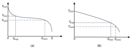
Figure 1.
Typical discharge curves of: (a) LFP cell; (b) NMC cell.
In addition, the cell internal resistance is needed, which is generally given in the datasheet. It should be noted that the discharge curves are obtained with a constant current discharge. Once all the data has been obtained, Equation (2) can be rewritten for each of the identified points to write a set of three equations with three unknowns .
At the start of the characteristic , the supplied charge is , the filtered current is , and the cell current is . Equation (2) gives:
The parameter , which represents the time constant of the exponential term, depends on the shape of the discharge curve. For the discharge curve of Figure 1a, it can be noticed that the exponential term energy is almost zero and can be approximated to 4. For the discharge curve of Figure 1b, the exponential term is still predominant and the parameter can be approximated to . For the exponential point, the voltage is , the supplied charge is , and the filtered current is because it is assumed that steady state has been reached. With the previous assumption, Equation (2) gives:
For the end of the nominal zone, the voltage is , the supplied charge is and Equation (2) gives:
Solving the set of Equations (4)–(6) gives the models parameters, which can be expressed as
where:
- ;
- ;
- ;
- ;
The parameter estimation procedure described above is now applied to the LG 18650HG2 cell. Figure 2a shows the extracted points from the datasheet discharge curves. Among the four characteristics, the one at 0.2 C was chosen for the parameter estimation procedure. Figure 2b–d shows the point identification on the 0.2 C discharge curves. Figure 2a depicts the maximum charge voltage and the maximum capacity Figure 2b,c represent respectively the exponential zone and the nominal zone detection.
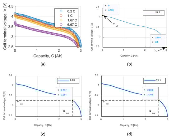
Figure 2.
(a) Points extracted from the datasheet discharge curves, at four different C rates (0.2 C, 1 C, 1.67 C, 6.67 C); Point identification for: (b) fully charged voltage and maximum cell capacity ; (c) Exponential zone voltage and capacity identification; (d) Nominal zone voltage and capacity identification.
Table 1 summarizes the identified points and the cell internal resistance given in the manufacturer’s datasheet. To estimate the other parameters, first a value for must be chosen looking at the shape of the discharge curve, as described in Section 2.1. In this case, was chosen. Using the data from Table 1 and the Equations (7)–(10), the model parameters, summarized in Table 2, were obtained.

Table 1.
Identified points for the parameter estimation procedure.
Table 2.
Shepherd model parameters.
2.2. Rint Model
A basic equivalent circuit battery model is shown Figure 3, and it is known as Internal Resistance Model or Rint model. This model describes the battery behavior using an ideal voltage source , whose purpose is to simulate the battery open circuit voltage, and a resistor that takes into account the battery internal resistance due to the electrodes [33]. The battery terminal voltage can be expressed as:
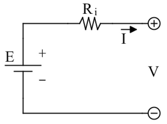
Figure 3.
Schematic representation of the Rint equivalent circuit model.
In this model, and are considered constant and the battery capacity is considered infinite. It can be used in simulation where the variation of the SoC is negligible.
Higher accuracy can be achieved by adding the SoC dependence for the open circuit voltage and the internal resistance.
To fully parametrize the model, and are needed. One of the advantages of this model is the possibility to parametrize it taking only the information from a typical cell manufacturer’s datasheet. Moreover, to consider the dependency of the battery capacity with the discharge current, the Peukert equation is used.
Normalization
The first step to parametrize the model is the extraction of the discharge curves from the datasheet. The discharge curves give the cell terminal voltage as a function of the supplied capacity, expressed in Ah, for different values of the discharge current. The discharge curves are then normalized and interpolated to have datasets with equally spaced grids. To achieve normalization, the capacity values are divided by their maximum values:
where the subscript is the considered discharge curve C-rate, and is the maximum capacity of the considered discharge curve. In this way, the discharge curves are represented as function of the Depth of Discharge (DoD).
Internal Resistance
The internal resistance as function of DoD can be derived from the normalized discharge curves, considering two different characteristics
If the internal resistance does not depend on the discharge current, it can be calculated as
Since usually N discharge curves are available in the datasheets, Equation (15) can be applied to all the curves combination. The internal resistance used in the model is finally calculated as the average value
where J is the number of possible combinations, given by
Open circuit voltage
The open circuit voltage as a function of DoD can be estimated as
Applying Equation (18) to all the discharge curves available in the datasheet, the average open circuit voltage as a function of the DoD is derived as
Capacity
The cell capacity depends on the discharge current, and to consider this phenomenon, the Peukert Capacity is considered [34,35]. If the battery supplies a current to the load, from the point of view of the battery capacity, it is as if a current equal to was supplied. If the battery is recharged, the phenomenon is negligible, therefore Accordingly, an equivalent battery capacity, defined as Peukert capacity, can be calculated as
where:
- is the Peukert Capacity (Ah);
- is the Peukert coefficient (-);
- is the discharge current (A);
- is the discharge time for discharge current (h).
To estimate the Peukert coefficient for a given cell, the discharge times at two different discharge currents are needed. From the manufacturer datasheet, the actual supplied capacity and the discharge current can be extrapolated, and the discharge time can be calculated as
And the Peukert coefficient is given by
From (22), the Peukert coefficient can be derived for any different discharge curves included in the datasheet. Usually, is chosen equal to the minimum discharge current while is varied to consider all the discharge profiles. The Peukert coefficient used for the simulation is then given by the average value as
The parameter estimation procedure described above is now applied to the LG18650HG2 cell. Figure 4a shows the datasheet discharge curve, which is given as a function of the supplied capacity. The curves are then normalized, using Equation (13), and interpolated as shown in Figure 4b. The internal resistance is estimated for each possible curve combination using Equation (15), obtaining the solid curves represented in Figure 5a. Finally, using Equation (16), the average internal resistance, represented in Figure 5b with the crossed line, is obtained.
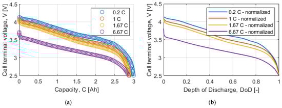
Figure 4.
Datasheet discharge curves: (a) extracted point from datasheet; (b) interpolated and normalized discharge curves.
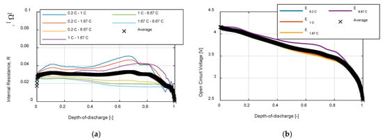
Figure 5.
Model parameter identification: (a) internal resistance and (b) open circuit voltage as a function of the Depth of Discharge.
The open circuit voltage is calculated for each discharge curve using Equation (18), represented in Figure 5b with the solid lines. The average open circuit voltage, shown in Figure 5b with the crossed line, is then obtained with Equation (19). Table 3 summarizes the Rint model parameters.
Table 3.
Rint model parameters.
2.3. Thevenin Model
The Rint model does not consider the transient behavior of the battery. The insertion of a parallel Resistor-Capacitor (RC) branch, as shown in Figure 6, allows considering the short-term transient due to the electrolyte polarization. Similarly to Rint model, E and represent respectively the battery open circuit voltage and the electrode resistance, represents the polarization resistance and represents the polarization capacitance [33]. To enhance the model accuracy and consider transient phenomenon with different time constants, other RC branches can be included in series with Thevenin’s model. However, the parameterization process of the model becomes even more complicated. If the model is employed to simulate the battery behavior in one operating condition at a given SoC, the model’s parameters can be counted as constants. Otherwise, if wide SoC operating range has to be simulated, the parameters can be considered dependent on temperature and SoC. The model is defined by the next equations:
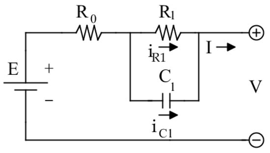
Figure 6.
Schematic representation of the Thevenin equivalent circuit model.
To fully parametrize the model, four parameters are needed: and they are all SoC dependent. For this model, the manufacturer’s specifications do not provide enough information to proceed with the parametrization procedure. Thus, some experimental tests must be performed, in particular a Pulse Discharge Test (PDT) [36]. The PDT consists in discharging a fully charged cell with a current pulse of specified amplitude and duration. At the end of the pulse, the cell is left in open circuit to stay at rest. At the end of the rest period, another current pulse is applied, and the procedure is repeated until the cell reaches the cut-off voltage.
The test starts charging the cell to its maximum voltage using the Constant Current/Constant Voltage procedure. After a rest period, the Pulse Discharge test is performed. The cell voltage is continuously acquired, and a pre-defined current pulse is applied. The removed charge in Ah can be calculated as:
Figure 7 illustrates the current pulse and the cell voltage, with all the equations used for the parameter estimation. At the start of the test, the acquired voltage corresponds to the cell open circuit voltage at 0% Depth of Discharge, due to the rest period after the full charge. The acquired voltage at the end of the rest period of the first current pulse, corresponds to the cell open circuit voltage at Depth of Discharge, where is the nominal capacity of the cell.
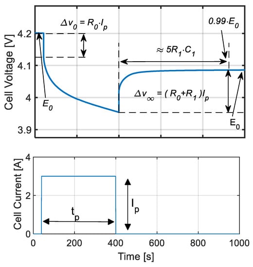
Figure 7.
Current pulse and battery terminal voltage response.
The immediate voltage reduction after the start of the current pulse is
And the internal resistance can be estimated as
Then, the cell is left open circuit for as long as it takes for the electrolyte polarization phenomenon to complete. The voltage rise, from end of the current pulse to the end of the rest period, is:
From the Equations (27) and (28), can be computed as:
Finally, the polarization capacitance is estimated considering that, after approximately five time constants, the cell terminal voltage is equal to , thus
And can be estimated as:
The parameter estimation procedure described above is now applied to the LG 18650HG2 cell. First, the characteristics of the current pulse are chosen. The pulse starts after 40 s from the beginning of the test, with an amplitude for . The removed charge is therefore
Corresponding to approximately 10% of the nominal capacity of the battery.
Figure 8 shows the experimental cell terminal voltage, acquired during the PDT, and used for the parameter estimation procedure. A MATLAB application was created to programmatically estimate all the parameters. The application considers each pulse individually and applies Equations (25)–(32) to calculate The results are reported in Figure 9, in which the red crosses are the estimated points and the blue solid line is a polynomial function, obtained with a least square approximation procedure. Table 4 summarizes the Thevenin model parameters.
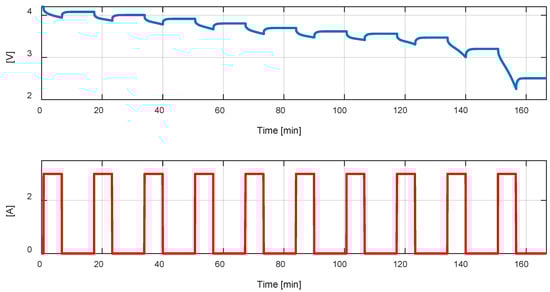
Figure 8.
Cell terminal voltage and battery current during the experimental PDT.
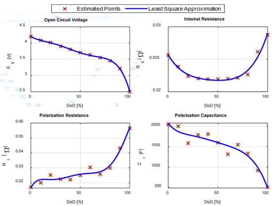
Figure 9.
Estimated parameters for the LG HG2 cell.
Table 4.
Thevenin model parameters.
3. Test-Bench Description
With the aim to validate experimentally the described models, a test bench (Figure 10) was implemented, composed of:
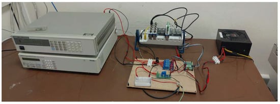
Figure 10.
Test-bench used for parameter estimation and model validation.
- a LG18650HG2 cell, whose characteristics are reported in Table 5;
Table 5. LG 18650HG2 cell Specification.
- a Fluke PM2812 Programmable Power Supply, whose characteristics are reported in Table 6, used to charge the cells;
Table 6. Power Supply Fluke PM2812 Specifications.
- an Agilent 6060B Single Input Electronic Load, whose characteristics are reported in Table 7, used on the discharge phase of the cell;
Table 7. Electronic Load Agilent 6060B Specifications.
- a NI 9215 16-Bit Data Acquisition Board (placed in a NI cDAQ 9172 chassis), whose characteristics are reported in Table 8, used to acquire the cell voltage signal;
Table 8. Data Acquisition Board NI 9215 Specifications.
- a SRD05VDCSl-C 4-Channels Optical Isolated Relay;
- a NI 9401 Digital Module (placed in the NI cDAQ 9172 chassis), used to control the relay.
All the instrumentation is controlled by a PC connected to the power supply and the electronic load via GPIB and to the NI chassis via USB.
The cell voltage signal is acquired at a 10 kS/s sampling frequency and then scaled at a 10 S/s sampling frequency calculating the average value in a 0.1 s time window. All the acquisitions were carried out after the calibration of the board.
The battery current is not directly measured and its values are taken from the values settled in the power supply (during the charge phase) or in the electronic load (during the discharge phase).
The battery capacity is estimated using the Coulomb Counting method, as:
where is the battery current, and is the sampling period.
Measurement Uncertainty Evaluation
In order to assess the accuracy of the parameters estimation for the Thevenin model, the uncertainty evaluation was performed, strictly following the rules prescribed by [37], for the measurements of the four parameters , , and .
The acquired voltage is affected by three main error sources, namely offset error, gain error and noise. The first step is to evaluate the uncertainty associated with each error source starting from the data acquisition board specifications:
- considering a recutangular distribution for the offset error;
- considering a rectangular distribution for the gain error and considering the worst case that corresponds to the maximum measured value (4.2 V);
- considering a gaussian distribution for the noise and considering that each measured values is the mean of 1000 acquired samples.
Therefore, the voltage standard uncertainty is
And the expanded uncertainty with a 99% confidence level (coverage factor k = 2.58) is, therefore, equal to 2.6 mV.
Actually, for the estimation of , and , only the differential voltage value is needed. In this case, the offset errors do not generate uncertainty, and, therefore:
And the expanded uncertainty is therefore equal to 1.3 mV.
With regard to the current measurement, starting from the electronic load specifications, three error sources have to be considered:
- considering a rectangular distribution for the offset error;
- considering a rectangular distribution for the gain error and considering the worst case that corresponds to the maximum measured value (5 A);
- the noise error is expressed as rms value.
Therefore, the current standard uncertainty is
The expanded uncertainty with a 99% confidence level is, therefore, equal to 91 mA.
Regarding the measurement, applying the uncertainty propagation low to Equation (27) and considering that the current during the parametrization process is set at 3 A, and the worst case, which corresponds to the maximum observed ()
The expanded uncertainty with a 99% confidence level is, therefore, equal to .
About the measurement, applying the uncertainty propagation low to Equation (29)
And the expanded uncertainty is therefore equal to .
Regarding the measurement, applying the uncertainty propagation low to Equation (31)
However, considering the low value of time jitter of the data acquisition board, the uncertainty of the measurement can be safely neglected. Therefore:
And the expanded uncertainty is therefore equal to .
With regard to the SoC measurement, referring to Equation (33)
That, neglecting the uncertainty and considering that the are constant (0.1 s) and considering steps, becomes
4. Validation of Models
The considered models are first validated by superimposing simulation results to the datasheet curves for the LG 18650HG2 Li-ion cell in Section 4.1. The models are then validated with respect to experimental results in different operating conditions in Section 4.2, Section 4.3 and Section 4.4. In particular, the constant current/constant voltage (CC/CV) recharge, the Pulse Discharge Test (PDT) and the Dynamic Discharge Test (DDT) of the cell are considered. In order to compare the models, the instantaneous error and the Root Mean Square Error (RMSE) expressed are considered. The instantaneous error is calculated as
where:
- is the actual value at the considered instant ;
- is the simulated value at the considered instant ;
- is the maximum observed value.
The Root Mean Square Error (RMSE) is calculated as
where:
- is the experimental value at the considered instant ;
- is the simulated vale at the considered instant ;
- is the number of samples of the experimental and simulated data.
4.1. Datasheet Discharge Curves
In the following sections, the described models are validated at steady state, comparing the discharge curves extracted from the manufacturer’s datasheet and the simulation results for the LG HG2 18,650 cells.
4.1.1. Shepherd Model Validation
Figure 11 shows the simulation results for the Shepherd model superimposed on the datasheet curves for different C-rates. The dotted curves represent the datasheets extracted points; the solid line represents the simulation results. It can be noted that, for lower C-rates (0.2 C, 1 C, 1.67 C), the simulated curves fit well to the datasheet curves during almost 85% of the discharge. For higher C-rate (6.67 C) this model does not give a good approximation of the cell voltage. The parameter estimation was done for the 0.2 C discharge curve, considering the parameters independent of the discharge current. In practice, the parameters also depend on the discharge current, and this can cause the accuracy problem.
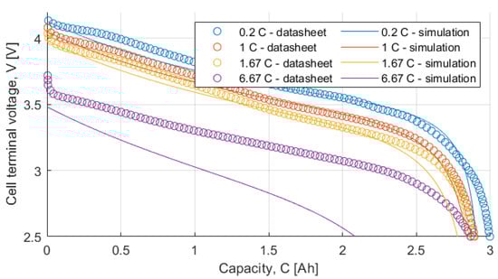
Figure 11.
Datasheet discharge curves vs. simulation results for the Shepherd model.
Figure 12 shows each discharge curve individually and the related instantaneous error calculated with Equation (49), and RMSE calculated with Equation (50). For 0.2 C, 1 C, 1.67 C discharge rates represented respectively in Figure 12a–c, the error is within 0–5% for SoC and within 100–20%. For SoC below 20%, the accuracy of the model decreases significantly. For 6.67 C discharge rate, represented in Figure 12b, the error starts at 4% and ramps up to 12%, hence this model is not suitable for high discharge rate.
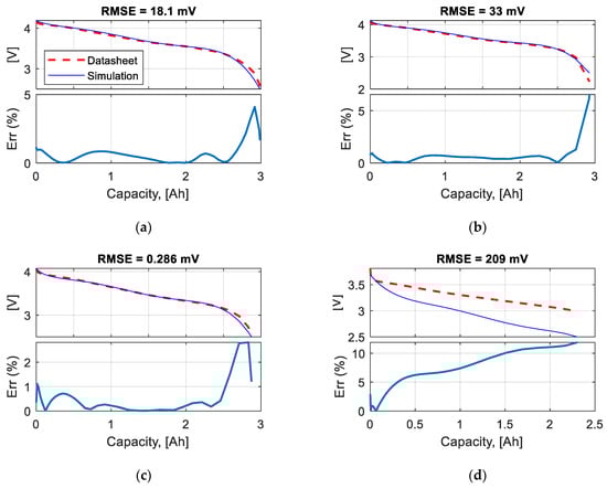
Figure 12.
Shepherd model datasheet vs. simulation curves and error: (a) 0.2 C discharge; (b) 1 C discharge; (c) 1.67 C discharge; (d) 6.67 C discharge.
4.1.2. Rint Model Validation
Figure 13 shows the simulation results for the Rint model superimposed on the datasheet curves for different C-rates. Similarly, to the Shepherd model, for lower C-rates (0.2 C, 1 C, 1.67 C), the model has better accuracy, but in this case also for the higher C-rate the model can predict with appropriate precision the cell terminal voltage.
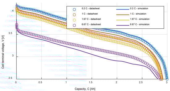
Figure 13.
Datasheet discharge curves vs. simulation results for the Rint model.
Figure 14 shows each discharge curve individually and the related error. For the 0.2 C discharge curve, Figure 14a, the error is below 1% for all the SoC range. For the 1 C discharge curve, Figure 14b, the error is below 5% for SoC between 100 to 20% but then starts to increase. For the 1.67 C discharge curve, Figure 14c is always below 2%. Finally, for the 6.67 C discharge curve, Figure 14d, the error is below 5%.
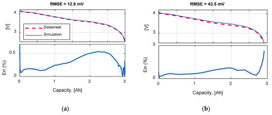
Figure 14.
Rint model datasheet vs. simulation curves and error: (a) 0.2 C discharge; (b) 1 C discharge; (c) 1.67 C discharge; (d) 6.67 C discharge.
4.1.3. Thevenin Model Validation
Figure 15 shows the simulation results for the Thevenin model superimposed on the datasheet curves for different C-rates. Again, the model has better accuracy for lower C-rates.
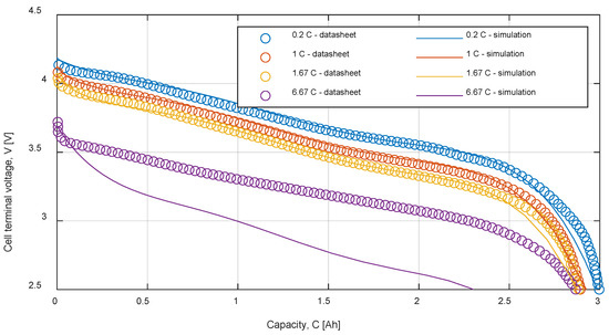
Figure 15.
Datasheet discharge curves vs. simulation results for the Thevenin model.
Figure 16 shows each discharge curve individually and the related error, calculated again with Equation (49). For the 0.2 C, 1 C and 1.67 C discharge curves, Figure 16a–c, similar results are obtained with an error below 2.5% for SoC between 100 to 20%. Finally, for the 6.67 C discharge curve, Figure 16d, the error continuously increases, thus this model is not suited for higher C-rates.
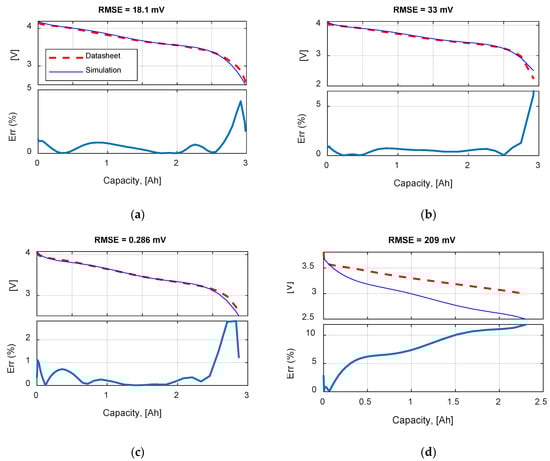
Figure 16.
Thevenin model datasheet vs. simulation curves and error for the Thevenin model: (a) 0.2 C discharge; (b) 1 C discharge; (c) 1.67 C discharge; (d) 6.67 C discharge.
4.2. Battery CC/CV Charge
Figure 17, Figure 18 and Figure 19a show the experimental cell voltage and current (solid blue and orange line respectively) superimposed to the simulated cell voltage and current (dashed blue and orange line respectively) obtained with the Shepherd, Rint and Thevenin model respectively. Figure 17, Figure 18 and Figure 19b show the instantaneous percentage error (solid blue line) and report the RMSE. The best results were obtained with the Thevenin model with a RMSE equal to 69 mV and an instantaneous error between most of the time.
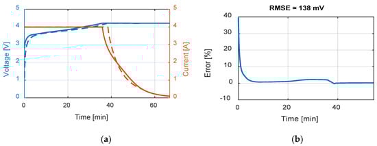
Figure 17.
Shepherd model CC/CV recharge: (a) experimental (solid line) and simulated (dashed line) voltage and current; (b) Error trend and RMSE.
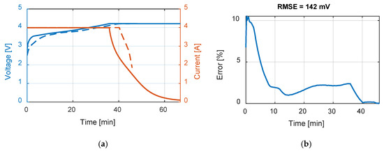
Figure 18.
Rint model CC/CV recharge: (a) experimental (solid line) and simulated (dashed line) voltage and current; (b) Error trend and RMSE.
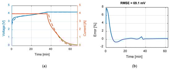
Figure 19.
Thevenin model CC/CV recharge: (a) experimental (solid line) and simulated (dashed line) voltage and current; (b) Error trend and RMSE.
4.3. Battery Pulse Discharge
Figure 20, Figure 21 and Figure 22a show the experimental cell voltage (solid blue line) and the simulated cell voltage (dashed orange line) obtained with the Shepherd, Rint and Thevenin model respectively for the Pulse Discharge Test. Figure 20, Figure 21 and Figure 22b show the instantaneous percentage error (solid blue line) and report the RMSE. Once again, the model that best fits the experimental results is the Thevenin model, with a RMSE equal to 15 mV and an instantaneous error between .
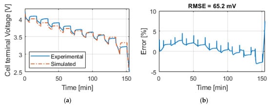
Figure 20.
Shepherd model Pulse Discharge Test: (a) experimental and simulated cell voltage; (b) Error trend and RMSE.
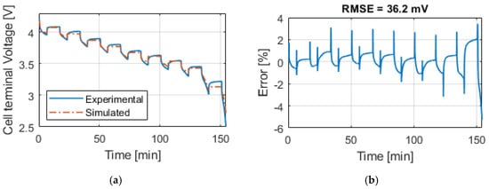
Figure 21.
Rint model Pulse Discharge Test: (a) experimental and simulated cell voltage; (b) Error trend and RMSE.
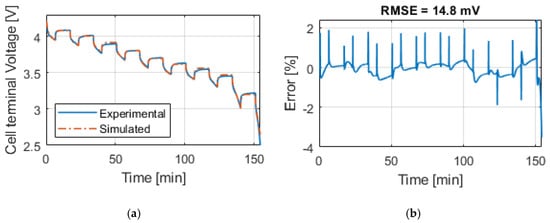
Figure 22.
Thevenin model Pulse Discharge Test: (a) experimental and simulated cell voltage; (b) Error trend and RMSE.
4.4. Battery Dynamic Discharge
Figure 23, Figure 24 and Figure 25a show the experimental cell voltage (solid blue line) and the simulated cell voltage (dashed orange line) obtained with the Shepherd, Rint and Thevenin model respectively for the Dynamic Discharge Test. Figure 23, Figure 24 and Figure 25b show the instantaneous percentage error (solid blue line) and report the RMSE. In this case too, the Thevenin model gives the best results with a RMSE equal to 44 mV and instantaneous error less than 3%.
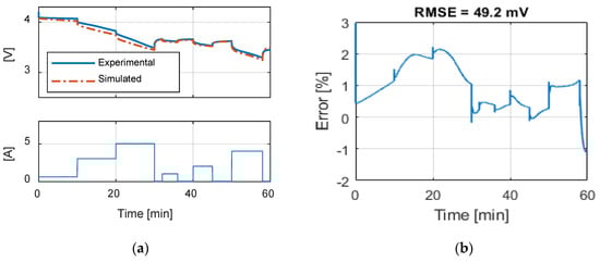
Figure 23.
Shepherd model Pulse Discharge Test: (a) experimental and simulated cell voltage; (b) Error trend and RMSE.
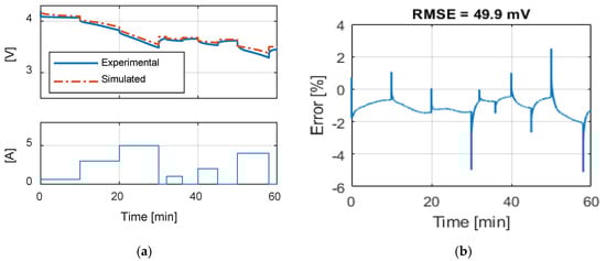
Figure 24.
Rint model Pulse Discharge Test: (a) experimental and simulated cell voltage; (b) Error trend and RMSE.
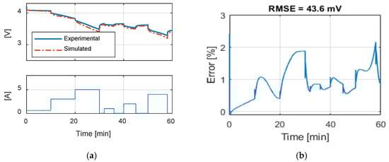
Figure 25.
Thevenin model Pulse Discharge Test: (a) experimental and simulated cell voltage; (b) Error trend and RMSE.
5. Discussion
This article carried out a comparison study of battery modeling and parameter identification techniques. Three models were considered: the Shepherd, the Rint and the Thevenin battery models. The Shepherd model belongs to the category of mathematical models. It can simulate the battery behavior both in static and transient operations thanks to the filtered current term. The parametrization procedure is quite simple, because all the necessary information can be found in the battery datasheet. The parametrization was carried out considering the 0.2 C discharge curve characteristic and considering the parameters current-independent.
The Rint model belongs to the category of equivalent circuit models and it does not consider the short-term battery dynamics. The parametrization procedure is a bit more complex than the Shepherd model one, but all the information can still be found in the manufacturer’s datasheet. The parametrization procedure considers different discharge curves, thus obtaining parameters that are somehow current dependent.
The Thevenin model belongs to the category of equivalent circuit models and, thanks to the RC branch, it can simulate the short-term battery dynamics. To parametrize the model, costly and time-consuming tests are required.
Table 9 summarizes the RMSE, expressed in mV, for all the model and test combinations. The bold numbers highlight the minimum obtained RMSE. It can be noticed that, considering the datasheet curves, the models can describe well the behavior of the battery for 0.2, 1 and 1.67 C. For 6.67 C (20 A), the best results were obtained with the Rint model. The Thevenin model gives the best results in all the experimental tests in terms of RMSE, but both the Sheperd and Rint models give adequate simulation results.
Table 9.
RMSE [mV] comparison.
The Sheperd and Rint models can be therefore used in early design phase, for example for a rough comparison between different types of cells, considering nominal voltage, weight, cost, overall dimensions, and quickly evaluating the performance of the battery pack. Once the cell type for the application is defined, the PDT can be performed to obtain the parameters for the Thevenin model, which gives better results in terms of accuracy. Moreover, the accuracy of the Thevenin model can be further improved by considering the parameters variable with current, temperature, age etc. by performing appropriate tests.
6. Conclusions
In this article, three battery equivalent circuit models (Shepherd, Rint, Thevenin) selected from the literature were presented and the parameters estimation procedures for each model were described. The parameters estimation procedures were systematically applied to the LG 18650HG2 battery cell. It should be noted that, for the Shepherd and Rint models, the parametrization can be carried out using just the information on manufacturer’s datasheets. However, their accuracy is limited by the veracity and precision of the curves and parameters in the datasheets. On the other hand, the Thevenin model requires a costly test-bench and time-consuming experimental test for its parametrization. The advantage, in this case, is the possibility to have a perfect knowledge of measurements and parameters estimation uncertainties. The comparison of the three models showed that Thevenin model, whose parameters were obtained from experimental tests, gave the best results as expected. However, the Shepherd and Rint models gave adequate simulation results, proving to be suitable for the early design stages of a battery-powered system. In this work, the temperature, battery current and ageing effect on the parameters were not considered, as this information would require expensive equipment and extensive testing. The aim of the work was to identify three easy-to-implement battery models, suitable for the early stages simulation and design of a battery-powered system. In the optimization phase of such systems, more accurate models should be used instead.
Author Contributions
Conceptualization, V.C.; Data curation, C.S., N.C. and V.C.; Investigation, V.C and C.S.; Methodology, V.C. and F.V.; Project administration, R.M., C.S. M.T. and R.A.M.; Software, V.C.; Supervision, F.V.; Validation, V.C.; Visualization, R.M. and V.C.; Writing—original draft, V.C.; Writing—review & editing, F.V. All authors have read and agreed to the published version of the manuscript.
Funding
This work was financially supported by PON R&I 2015–2020 “Propulsione e Sistemi Ibridi per velivoli ad ala fissa e rotante—PROSIB”, CUP no:B66C18000290005, by H2020-ECSEL-2017-1-IA-two-stage “first and european sic eightinches pilot line-REACTION”, by Prin 2017—Settore/Ambito di intervento: PE7 linea C—Advanced power-trains and -systems for full electric aircrafts, by PON R&I 2014-2020—AIM (Attraction and International Mobility), project AIM1851228-1 and by ARS01_00459-PRJ-0052 ADAS+ “Sviluppo di tecnologie e sistemi avanzati per la sicurezza dell’auto mediante piattaforme ADAS”; SDES (Sustainable Development and Energy Savings) Laboratory UNINETLAB of University of Palermo, Laboratory of Electrical APplications LEAP of University of Palermo.
Conflicts of Interest
The authors declare no conflict of interest.
References
- Saldaña, G.; San Martín, J.I.; Zamora, I.; Asensio, F.J.; Oñederra, O. Analysis of the Current Electric Battery Models for Electric Vehicle Simulation. Energies 2019, 12, 2750. [Google Scholar] [CrossRef]
- He, H.; Qin, H.; Sun, X.; Shui, Y. Comparison Study on the Battery SoC Estimation with EKF and UKF Algorithms. Energies 2013, 6, 5088. [Google Scholar] [CrossRef]
- Wang, D.; Bao, Y.; Shi, J. Online Lithium-Ion Battery Internal Resistance Measurement Application in State-of-Charge Estimation Using the Extended Kalman Filter. Energies 2017, 10, 1284. [Google Scholar] [CrossRef]
- Yang, H.; Qiu, Y.; Guo, X. Prediction of State-of-Health for Nickel-Metal Hydride Batteries by a Curve Model Based on Charge-Discharge Tests. Energies 2015, 8, 2322. [Google Scholar] [CrossRef]
- Gismero, A.; Schaltz, E.; Stroe, D.-I. Recursive State of Charge and State of Health Estimation Method for Lithium-Ion Batteries Based on Coulomb Counting and Open Circuit Voltage. Energies 2020, 13, 1811. [Google Scholar] [CrossRef]
- Samadani, S.E.; Fraser, R.A.; Fowler, M. A Review Study of Methods for Lithium-ion Battery Health Monitoring and Remaining Life Estimation in Hybrid Electric Vehicles. SAE Tech. Paper Ser. 2012. [Google Scholar] [CrossRef]
- Raszmann, E.; Baker, K.; Shi, Y.; Christensen, D. Modeling stationary lithium-ion batteries for optimization and predictive control. In Proceedings of the 2017 IEEE Power and Energy Conference at Illinois (PECI), Champaign, IL, USA, 23–24 February 2017; pp. 1–7. [Google Scholar]
- Jongerden, M.R.; Haverkort, B.R.H.M. Battery Modeling; Design and Analysis of Communication Systems (DACS): Enschede, The Netherlands, 2008. [Google Scholar]
- Fotouhi, A.; Auger, D.J.; Propp, K.; Longo, S.; Wild, M. A review on electric vehicle battery modelling: From Lithium-ion toward Lithium–Sulphur. Renew. Sustain. Energy Rev. 2016, 56, 1008–1021. [Google Scholar] [CrossRef]
- Barcellona, S.; Piegari, L. Lithium Ion Battery Models and Parameter Identification Techniques. Energies 2017, 10, 2007. [Google Scholar] [CrossRef]
- Damiano, A.; Porru, M.; Salimbeni, A.; Serpi, A.; Castiglia, V.; Di Tommaso, A.O.; Miceli, R.; Schettino, G. Batteries for Aerospace: A Brief Review. In Proceedings of the 2018 AEIT International Annual Conference, Bari, Italy, 3–5 October 2018; pp. 1–6. [Google Scholar]
- Doyle, M.; Fuller, T.F.; Newman, J. Modeling of Galvanostatic Charge and Discharge of the Lithium/Polymer/Insertion Cell. J. Electrochem. Soc. 1993, 140, 1526. [Google Scholar] [CrossRef]
- Fuller, T.F.; Doyle, M.; Newman, J. Simulation and Optimization of the Dual Lithium Ion Insertion Cell. J. Electrochem. Soc. 1994, 141, 1. [Google Scholar] [CrossRef]
- Newman, J.; Tiedemann, W. Porous-electrode theory with battery applications. AIChE J. 1975, 21, 25–41. [Google Scholar] [CrossRef]
- Smith, K.; Wang, C.-Y. Solid-state diffusion limitations on pulse operation of a lithium ion cell for hybrid electric vehicles. J. Power Sources 2006, 161, 628–639. [Google Scholar] [CrossRef]
- Ahmed, R.; Sayed, M.E.; Arasaratnam, I.; Tjong, J.; Habibi, S. Reduced-Order Electrochemical Model Parameters Identification and SOC Estimation for Healthy and Aged Li-Ion Batteries Part I: Parameterization Model Development for Healthy Batteries. IEEE J. Emerg. Sel. Top. Power Electron. 2014, 2, 659–677. [Google Scholar] [CrossRef]
- Ahmed, R.; Sayed, M.E.; Arasaratnam, I.; Tjong, J.; Habibi, S. Reduced-Order Electrochemical Model Parameters Identification and State of Charge Estimation for Healthy and Aged Li-Ion Batteries—Part II: Aged Battery Model and State of Charge Estimation. IEEE J. Emerg. Sel. Top. Power Electron. 2014, 2, 678–690. [Google Scholar] [CrossRef]
- Fan, G.; Li, X.; Canova, M. A Reduced-Order Electrochemical Model of Li-Ion Batteries for Control and Estimation Applications. IEEE Trans. Veh. Technol. 2018, 67, 76–91. [Google Scholar] [CrossRef]
- Doyle, M.; Newman, J. The use of mathematical modeling in the design of lithium/polymer battery systems. Electrochim. Acta 1995, 40, 2191–2196. [Google Scholar] [CrossRef]
- Li, R.; Wang, Z.; Yu, J.; Lei, Y.; Zhang, Y.; He, J. Dynamic Parameter Identification of Mathematical Model of Lithium-Ion Battery Based on Least Square Method. In Proceedings of the 2018 IEEE International Power Electronics and Application Conference and Exposition (PEAC), Shenzhen, China, 4–7 November 2018; pp. 1–5. [Google Scholar]
- Haoran, L.; Liangdong, L.; Xiaoyin, Z.; Mingxuan, S. Lithium Battery SOC Estimation Based on Extended Kalman Filtering Algorithm. In Proceedings of the 2018 IEEE 4th International Conference on Control Science and Systems Engineering (ICCSSE), Wuhan, China, 21–23 August 2018; pp. 231–235. [Google Scholar]
- Li, S.; Ke, B. Study of battery modeling using mathematical and circuit oriented approaches. In Proceedings of the 2011 IEEE Power and Energy Society General Meeting, Detroit, MI, USA, 24–28 July 2011; pp. 1–8. [Google Scholar]
- Hinz, H. Comparison of Lithium-Ion Battery Models for Simulating Storage Systems in Distributed Power Generation. Inventions 2019, 4, 41. [Google Scholar] [CrossRef]
- Nikolian, A.; Firouz, Y.; Gopalakrishnan, R.; Timmermans, J.-M.; Omar, N.; Van den Bossche, P.; Van Mierlo, J. Lithium Ion Batteries—Development of Advanced Electrical Equivalent Circuit Models for Nickel Manganese Cobalt Lithium-Ion. Energies 2016, 9, 360. [Google Scholar] [CrossRef]
- Grandjean, T.R.B.; McGordon, A.; Jennings, P.A. Structural Identifiability of Equivalent Circuit Models for Li-Ion Batteries. Energies 2017, 10, 90. [Google Scholar] [CrossRef]
- He, H.; Xiong, R.; Guo, H.; Li, S. Comparison study on the battery models used for the energy management of batteries in electric vehicles. Energy Convers. Manag. 2012, 64, 113–121. [Google Scholar] [CrossRef]
- Barreras, J.V.; Schaltz, E.; Andreasen, S.J.; Minko, T. Datasheet-based modeling of Li-Ion batteries. In Proceedings of the 2012 IEEE Vehicle Power and Propulsion Conference, Seoul, Korea, 9–12 October 2012; pp. 830–835. [Google Scholar]
- Castiglia, V.; Livreri, P.; Miceli, R.; Pellitteri, F.; Schettino, G.; Viola, F. Power Management of a Battery/Supercapacitor System for E-Mobility Applications. In Proceedings of the 2019 AEIT International Conference of Electrical and Electronic Technologies for Automotive (AEIT AUTOMOTIVE), Torino, Italy, 2–4 July 2019; pp. 1–5. [Google Scholar]
- Potrykus, S.; Kutt, F.; Nieznański, J.; Fernández Morales, F.J. Advanced Lithium-Ion Battery Model for Power System Performance Analysis. Energies 2020, 13, 2411. [Google Scholar] [CrossRef]
- Shepherd, C.M. Design of Primary and Secondary Cells: II. An Equation Describing Battery Discharge. J. Electrochem. Soc. 1965, 112, 657. [Google Scholar] [CrossRef]
- Enache, B.; Lefter, E.; Stoica, C. Comparative study for generic battery models used for electric vehicles. In Proceedings of the 2013 8th International Symposium on Advanced Topics in Electrical Engineering (ATEE), Bucharest, Romania, 23–25 May 2013; pp. 1–6. [Google Scholar]
- Tremblay, O.; Dessaint, L.-A. Experimental Validation of a Battery Dynamic Model for EV Applications. World Electr. Veh. J. 2009, 3, 289. [Google Scholar] [CrossRef]
- Castiglia, V.; Miceli, R.; Ala, G.; Romano, P.; Viola, F.; Giglia, G.; Imburgia, A.; Schettino, G. Modelling, simulation and characterization of Li-Ion battery cell. In Proceedings of the 2019 IEEE 5th International Forum on Research and Technology for Society and Industry (RTSI), Florence, Italy, 9–12 September 2019; pp. 400–405. [Google Scholar]
- Doerffel, D.; Sharkh, S.A. A critical review of using the Peukert equation for determining the remaining capacity of lead-acid and lithium-ion batteries. J. Power Sources 2006, 155, 395–400. [Google Scholar] [CrossRef]
- Omar, N.; Bossche, P.V.d.; Coosemans, T.; Mierlo, J.V. Peukert Revisited—Critical Appraisal and Need for Modification for Lithium-Ion Batteries. Energies 2013, 6, 5625. [Google Scholar] [CrossRef]
- Plett, G.L. Modeling, Simulation, and Identification of Battery Dynamics. Available online: http://mocha-java.uccs.edu/ECE5710/index.html (accessed on 10 February 2020).
- JCGM 100. Evaluation of Measurement Data—Guide to the Expression of Uncertainty in Measurement. 2008. Available online: https://www.bipm.org/utils/common/documents/jcgm/JCGM_100_2008_E.pdf (accessed on 10 February 2020).


© 2020 by the authors. Licensee MDPI, Basel, Switzerland. This article is an open access article distributed under the terms and conditions of the Creative Commons Attribution (CC BY) license (http://creativecommons.org/licenses/by/4.0/).