Impact of Lossy Compression Techniques on the Impedance Determination

Abstract

One of the essential parameters to measure the stability and power-quality of an energy grid is the network impedance. Including distinct resonances which may also vary over time due to changing load or generation conditions in a network, the frequency characteristic of the impedance is an import part to analyse. The determination and analysis of the impedance go hand in hand with a massive amount of data output. The reduction of this high-resolution voltage and current datasets, while maintaining the fidelity of important information, is the main focus of this paper. The presented approach takes measured impedance datasets and a set of lossy compression procedures, to monitor the performance success with known key metrics. Afterwards, it continually compares the results of various lossy compression techniques. The innovative contribution is the combination of new and existing procedures as well as metrics in one approach, to reduce the size of the impedance datasets for the first time. The approach needs to be efficient, suitable, and exact, otherwise the decompression results are useless.

1. Introduction

The energy system transformation and smart grid applications require knowledge about detailed power and load profiles with sophisticated datasets on the one hand. On the other, an increasing number of power electronic converters (PECs) from renewable energies and smart loads are integrated into the electrical supply system to measure and analyse the power-quality, stability, and control design considerations. Since the first generation of grid-connected converters, the grid impedance has been an important part of the analysis of the stability of the whole energy system or detection of islanding grids [1,2]. The so-called PECs are usually self-controlled pulse width modulation (PWM) power converters that connect generators or loads to the 50 Hz power supply system. For the power-quality analysis or a filter design of the converters detailed knowledge is required of the frequency characteristics of the network impedance at a specific grid-connection point [3]. Along with the increasing number of PECs especially in low and medium voltage grids, the generated, and transferred amount of data rises massively. This opens up multiple situations for system optimization. The current operational conditions of the municipal utilities, grid owner, or system operator—low bandwidth and low computational power—and the development of impedance shaping intensifies problems in many cases [4,5]. To improve memory consumption, collection, and transmission efficiency, the reduction of high-resolution impedance datasets while maintaining the fidelity of relevant information presents one opportunity for system optimization.

The overwhelming majority of the studies that try to tackle this larger issue focus on how to generate, analyse, and shape the network impedance so as to make it usable with the grid [6,7,8]. As regards the topic of compression, some approaches have been investigated in the field of medical data science [9].

This paper addresses the question of how to compress voltage and current datasets of an impedance measurement device by using lossy compression approaches without any detrimental effect on the impedance results of the measurement. Since raw voltage and current datasets contain further information e.g., about voltage harmonics, the aim is to compress the raw data instead of the calculated impedance data. Therefore, the scope of the paper is the grid impedance and the compression compatibility. It is not important to compress the data set one-to-one or to create a method with the highest efficiency, depending on processing duration or error level. The idea is to generate an easy to handle, efficient, sufficiently selective, accurate, and usable approach that output a compressed impedance dataset without irrelevancies. Two other highly important questions are, one, how to transfer and store large amounts of data using small amounts of resources and costs and, two, how to extract necessary information from the dataset. Due to limited computational i.e., bandwidth and storage space, and human resources lossy compression algorithms are promising. The new procedure and model technique, which combines measured impedance datasets, lossy compression techniques, and key metrics addresses exactly this specific gap in knowledge.

Section 2 describes the background of the impedance measurement to show the used test case and the simulation approach, which produced the dataset. The remainder of this paper is organized as follows. Section 3 presents typical lossy compression approaches, which can be used to reduce the amount of data. After those techniques have been explained, the approach taken in this paper, and the key metrics are introduced in Section 4. The obtained performance results are presented in Section 5 to show if they meet the required criteria. Finally, conclusion and outlook are presented in Section 6.

2. Mid Voltage Impedance Measurement System

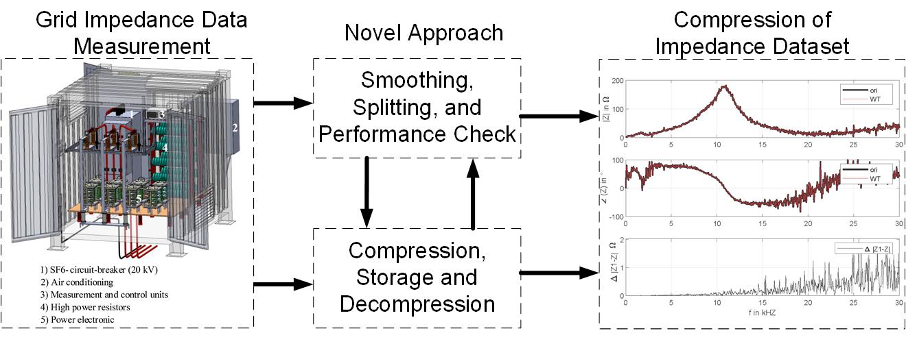
In the literature, the methods to measure the network impedance may be categorized into active and passive methods used for power systems during operation. Active methods use excitation signals at the point of common coupling (PCC) to identify the impedance. The signal generator can be a current or voltage source or a current sink.

2.1. Impedance Identification

The used signal generation is a sink: A load resistor is switched on and off in a random pattern. Hence, the load current is a random pulse pattern. Figure 1 shows the principle connection scheme of the network impedance measurement (NIM) device and its corresponding complex equivalent circuit. The voltage in off and on state ($v_1\left(t\right)$ and $v_2\left(t\right)$) as well as the current in the on state $i_2\left(t\right)$ (off state current $i_1\left(t\right)$ is zero) are measured. The frequency-dependent complex values ${\underline{V}}_1\left(\omega \right),{\underline{V}}_2\left(\omega \right)$ and ${\underline{I}}_2\left(\omega \right)$, derived from the fast Fourier transform, are used to calculate the complex frequency-dependent impedance ${\underline{Z}}_{\mathrm{N}}\left(\omega \right)$ (1).

$${\underline{Z}}_{\mathrm{N}}\left(\omega \right)=\frac{{\underline{V}}_2\left(\omega \right)-{\underline{V}}_1\left(\omega \right)}{{\underline{I}}_2\left(\omega \right)}$$

(1)

2.2. Impedance Identification of Three Phase Systems

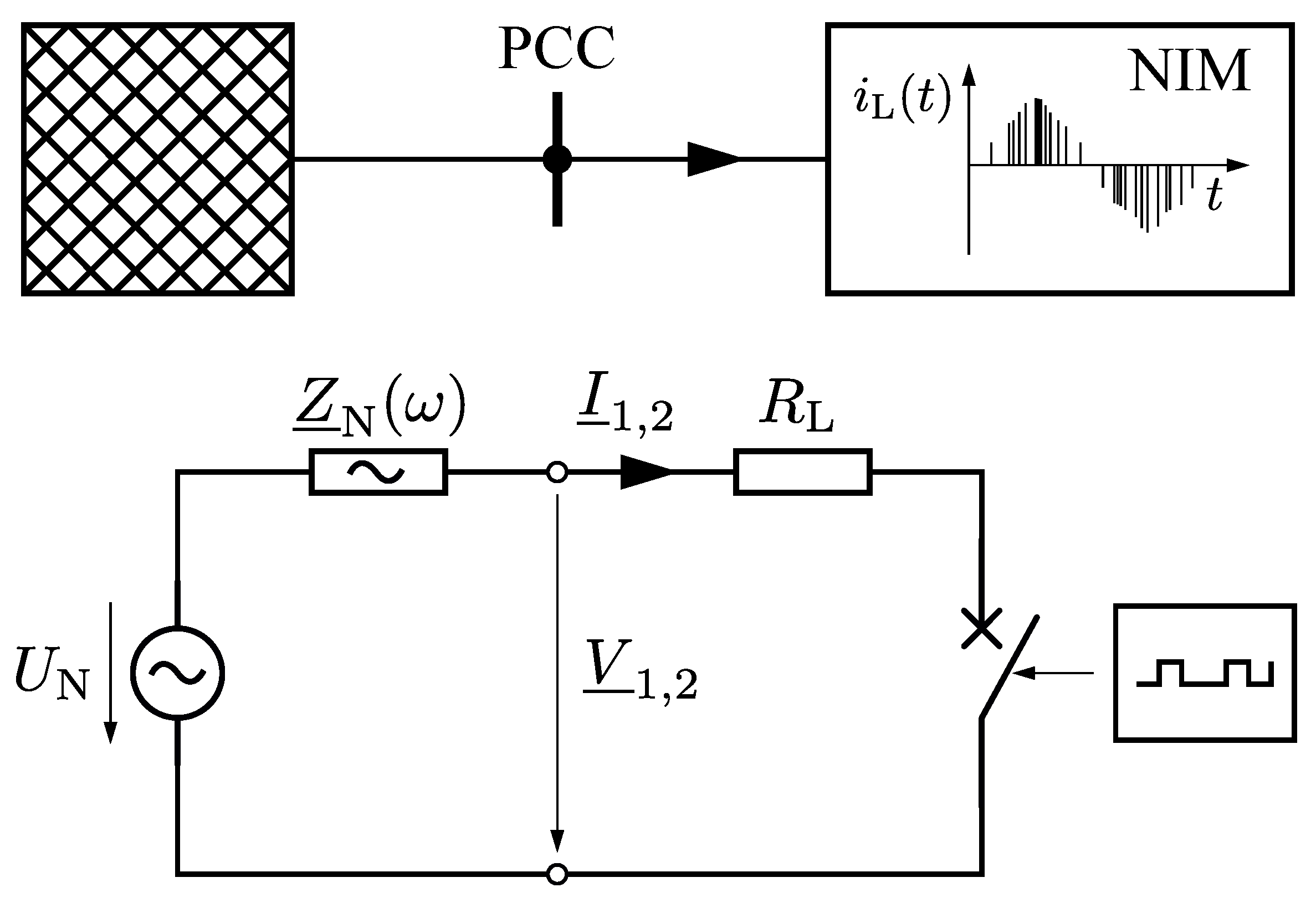
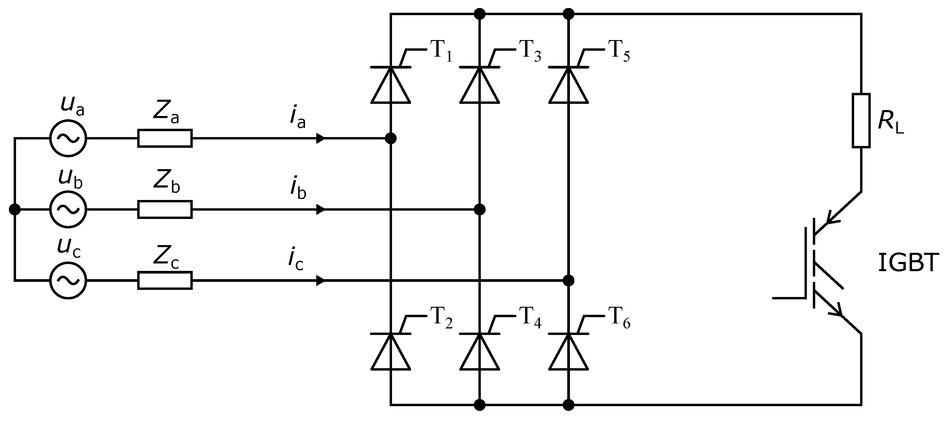
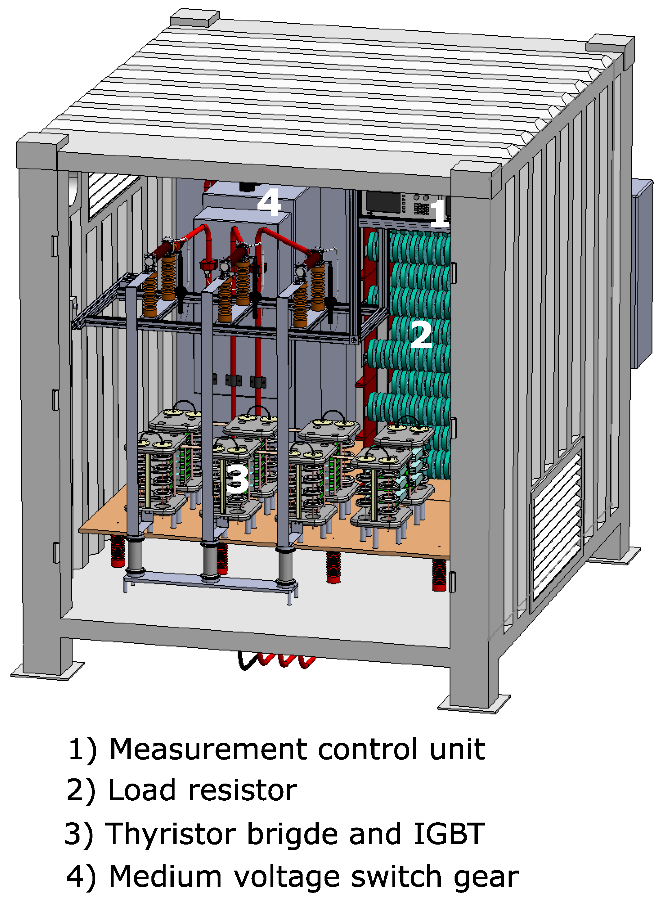
In this section, the measurement system for the determination of the frequency dependency of the grid impedance is presented. The device includes highly accurate sensors for the measurement of voltage and current wave forms. Figure 2 shows a simplified scheme of the measurement setup to evaluate the impedance of the three-phase mid voltage PCC [10,11]. A resistive load is switched by an insulated gate bipolar transistor (IGBT), while the measurement loop (e.g., L1–L2) is selected by a B6 thyristor bridge. A 3D model of the measurement device and its main components are depicted in Figure 3. The measurement device is portable and may be connected to connection points in medium voltage grids via its own medium voltage switch gear (SF6 circuit breaker). To determine the line impedances of a three-phase system four measurements are required:

• At first, the open circuit is measured to obtain the reference ${\underline{V}}_1\left(\omega \right)$. Hence, the load is not pulsed and ${\underline{I}}_1\left(\omega \right)$ is zero,
• Then, a pulse pattern is applied to the three loops of phase a to b, phase b to c, and phase c to a.

For each measurement the following parameters are recorded over at least one period of 50 Hz:

• $i_{\mathrm{a}}\left(t\right)$/$i_{\mathrm{b}}\left(t\right)$/$i_{\mathrm{c}}\left(t\right)$: current phase a/b/c
• $u_{\mathrm{a}}\left(t\right)$/$u_{\mathrm{b}}\left(t\right)$/$u_{\mathrm{c}}\left(t\right)$: voltage phase a/b/c to earth

The loop impedances ${\underline{Z}}_{\mathrm{ab}}\left(\omega \right)$, ${\underline{Z}}_{\mathrm{bc}}\left(\omega \right)$, ${\underline{Z}}_{\mathrm{ca}}\left(\omega \right)$ are derived from the recorded parameters with (1). These loop impedances can be rearranged into the line impedances ${\underline{Z}}_{\mathrm{a}}\left(\omega \right)$, ${\underline{Z}}_{\mathrm{b}}\left(\omega \right)$, and ${\underline{Z}}_{\mathrm{c}}\left(\omega \right)$ [10]:

$$\begin{array}{cc}\hfill {\underline{Z}}_{\mathrm{a}}\left(\omega \right)& =\frac{1}{2}·\left[{\underline{Z}}_{\mathrm{ab}}\left(\omega \right)-{\underline{Z}}_{\mathrm{bc}}\left(\omega \right)+{\underline{Z}}_{\mathrm{ca}}\left(\omega \right)\right]\hfill \end{array}$$

(2)

$$\begin{array}{cc}\hfill {\underline{Z}}_{\mathrm{b}}\left(\omega \right)& =\frac{1}{2}·\left[{\underline{Z}}_{\mathrm{ab}}\left(\omega \right)+{\underline{Z}}_{\mathrm{bc}}\left(\omega \right)-{\underline{Z}}_{\mathrm{ca}}\left(\omega \right)\right]\hfill \end{array}$$

(3)

$$\begin{array}{cc}\hfill {\underline{Z}}_{\mathrm{c}}\left(\omega \right)& =\frac{1}{2}·\left[-{\underline{Z}}_{\mathrm{ab}}\left(\omega \right)+{\underline{Z}}_{\mathrm{bc}}\left(\omega \right)+{\underline{Z}}_{\mathrm{ca}}\left(\omega \right)\right]\hfill \end{array}$$

(4)

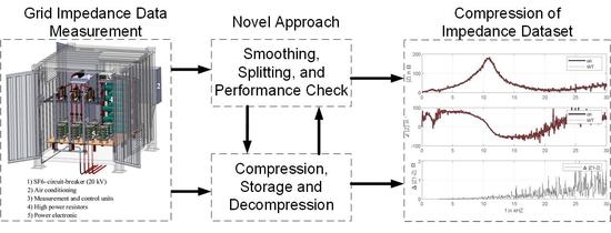
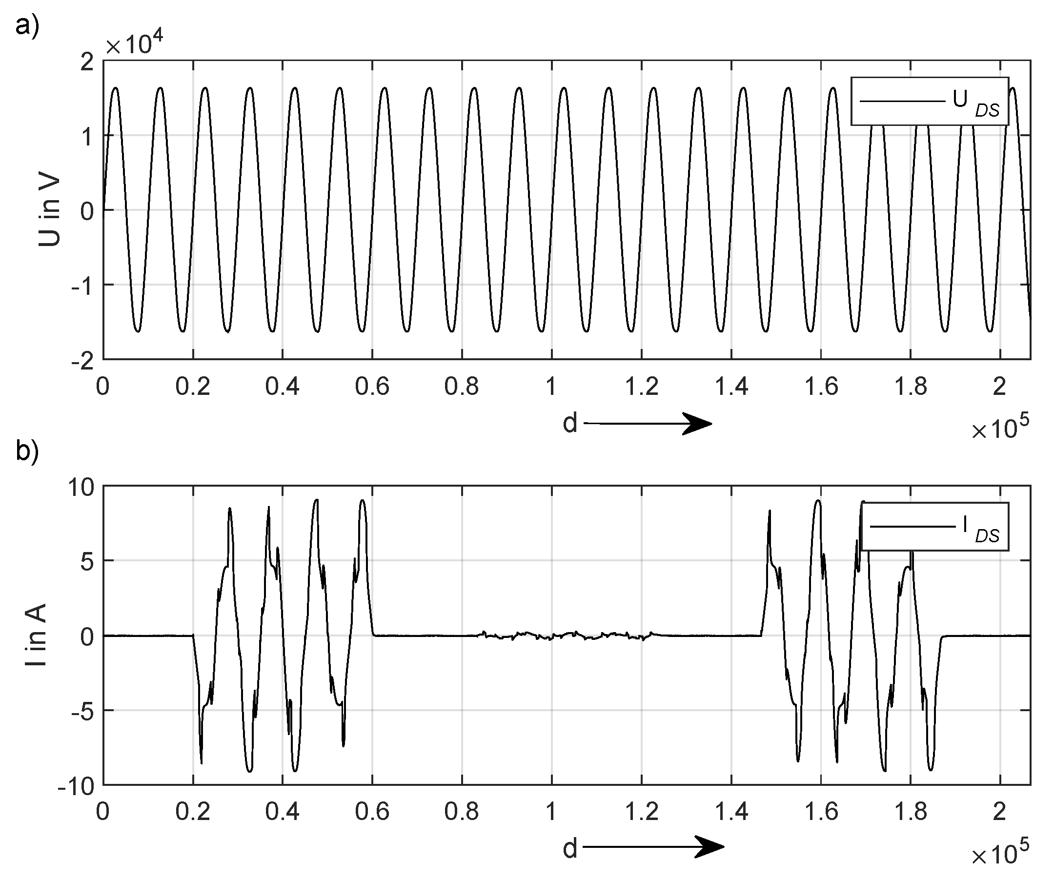
Typically, the impedances are average values over ten 50 $\mathrm{Hz}$ periods measured every five minutes over a month or more to identify impedance changes over daytime. Figure 4 shows a sample measurement. The compression approach, explained in Section 4, is applied to the voltage and current data, which is recorded during grid excitation and which is used for the calculation of the grid impedance. The authors want to determine the effect of data compression on the grid impedance calculation with this compressed raw dataset.

This setting yields 288 measurements per day or 8928 per month for each recorded voltage and current parameter. The sample rate is 500 $\mathrm{kHz}$. Overall, the authors use a dataset with d = 206,744 data points (sample size d) for each recorded parameter, voltage and current. For an easy representation of the following figures and the compression dataset, the number of measuring points d was used (instead of the time vector t). Theoretically, the respective t-vector would have to be multiplied by the reciprocal of the sampling rate (500 $\mathrm{kHz}$).

As the measurement device is remotely controlled and the data is transferred via the cellular network a compression is beneficial to optimize the data transfer speed and costs. Especially when the measurement device’s installation site is in areas with low network coverage exhibiting low transfer rates. The transients in the recorded voltage and current parameters are the essential part of the data, as they determine the frequency dependency of the impedance values.

3. Lossy Compression Techniques

Various meta-analyses, types and overviews of data compression approaches can be found in [12,13,14,15,16]. The compression techniques are divided into lossy and lossless methods. Lossy ones generate better results by losing (preferably irrelevant) information. This can be explained by the fact that the result of the decompression is not identical to the starting dataset. In contrast, lossless methods produce an identical decompressed dataset [13].

The combination of impedance measurements and data compression can hitherto be found only in other fields of research. As an example serves the medical area where an extensive comparison of compression methods adapted to the impedance of cardiomyocytes is presented. The approach uses the wavelet transformation technique to analyse the effect of compression on sensitive data coming from cardiomyocytes and generating compression ratio of round about 5:1 [9].

Hereinafter follows a short description of the lossy compression methods that are compared in this paper. All of these approaches are frequently used for other types of data (SVD, WT) and appear interesting for the paper approach (TFA) [17,18,19,20,21,22]. The two well-known, widely used approaches WT and SVD are only briefly described. For further explanation, please consult the references that are listed in the Section 3.1 and Section 3.2. TFA is explained in more detail but can be found in [17,22] if necessary.

3.1. SVD—Singular Value Decomposition

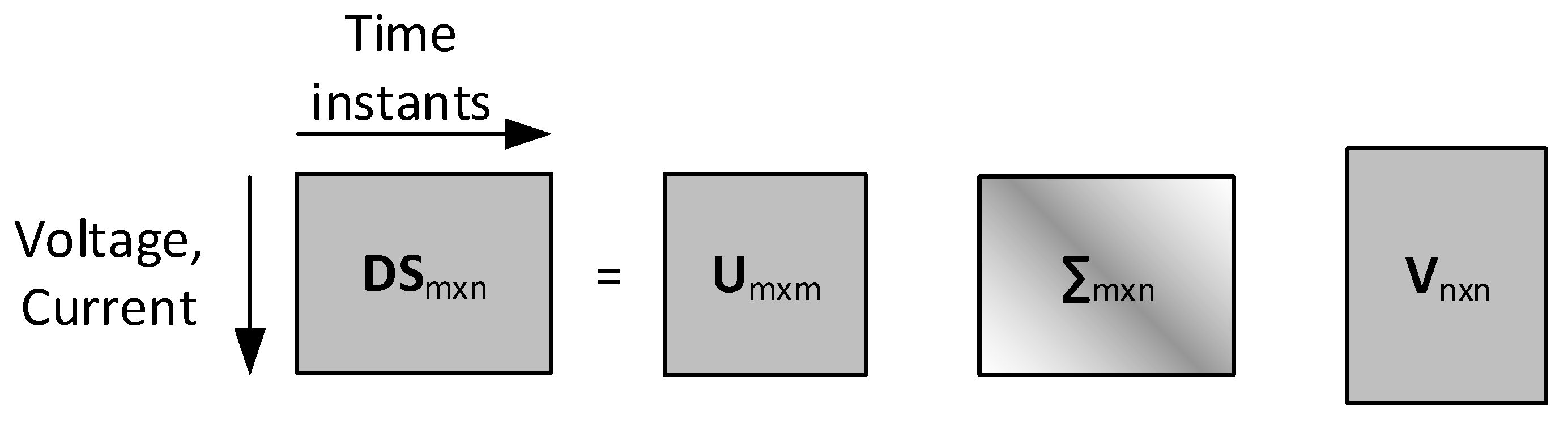
The so-called Singular Value Decomposition (SVD) splits a m × n set of data (voltage/current × time stamp) $\mathbf{DS}$ into three different matrices (5). The diagonal matrix $\mathsf{\Sigma }$ contains the singular values (SVs), see also Figure 5.

$$\begin{array}{ccc}\hfill {\mathbf{DS}}_{m\times n}& =& {\mathbf{U}}_{m\times m}{\mathsf{\Sigma }}_{m\times n}{\mathbf{V}}_{n\times n}^{\mathrm{T}}\hfill \end{array}$$

(5)

The data compression takes advantage of the fact that a close approximation of $\mathbf{DS}$ can be achieved by keeping the significant SVs of matrix $\mathsf{\Sigma }$. The compression success depends on the amount of reduction of singular values in $\mathsf{\Sigma }$.

3.2. WT—Wavelet Transformation

A wavelet transform (WT) orthogonally decomposes a time series into wavelet and scaling coefficients. The main difference to the Fourier transform, which splits a signal into cosine and sine, is the use of (real and Fourier space) functions by the WT. The deletion of irrelevant data points increase the compression ratio and reduce the mean percentage error (MPE) and mean absolute error (MAE). That is why, it is important to find the best thresholds, levels of decomposition (LoD), and Daubechies’ wavelets (DW). For further explanation, see [19,20,21].

3.3. TFA—Triangular Function Algorithm

The Triangular Function Algorithm (TFA) encloses the steps (I)–(VI) and is an enhanced version of the approach developed in [17]. (I) Read the dataset and choose your preferred percentiles (e.g., $Q_5$–$Q_{95}$). (II) Generate percentiles of the original dataset and save the data points $y_{\mathrm{iQ}}$, $x_{iQ}$. Perform a moving average FIR filter to smooth the (remainder of the) dataset. (III) Read $a_0$ data points, which is the step width. (IV) Choose number of polynomials of least square fit. Perform $\mathsf{\Lambda }$ in (6), to obtain the slope $b_1$ and intercept $b_0$ (6). Determine the mean square error and unbiased standard deviation ($\sigma$).

$$\begin{array}{ccc}\hfill \mathsf{\Lambda }& =& \sum _{i=1}^a{\left[y_i-\left(b_1{x}_i+b_0\right)\right]}^2\hfill \end{array}$$

(6)

In our case, quadratic or higher polynomial functions should be avoided because of the lower compression-error-ratio depending on the higher number of compressed and saved datapoints (e.g., $b_2$, $b_1$, $b_0$). (V) Read and check the following data point ($y_i$, $x_i$). If its value is within (±m$\sigma$, with factor m) the predicted values, jump to (III). Otherwise start a new line segment and go to step (IV). (VI) After compressing the whole dataset, insert percentiles ($y_{\mathrm{iQ}}$, $x_{iQ}$) to finish the algorithm. For further explanation, please see [17].

4. Proposed Approach and Key Metrics

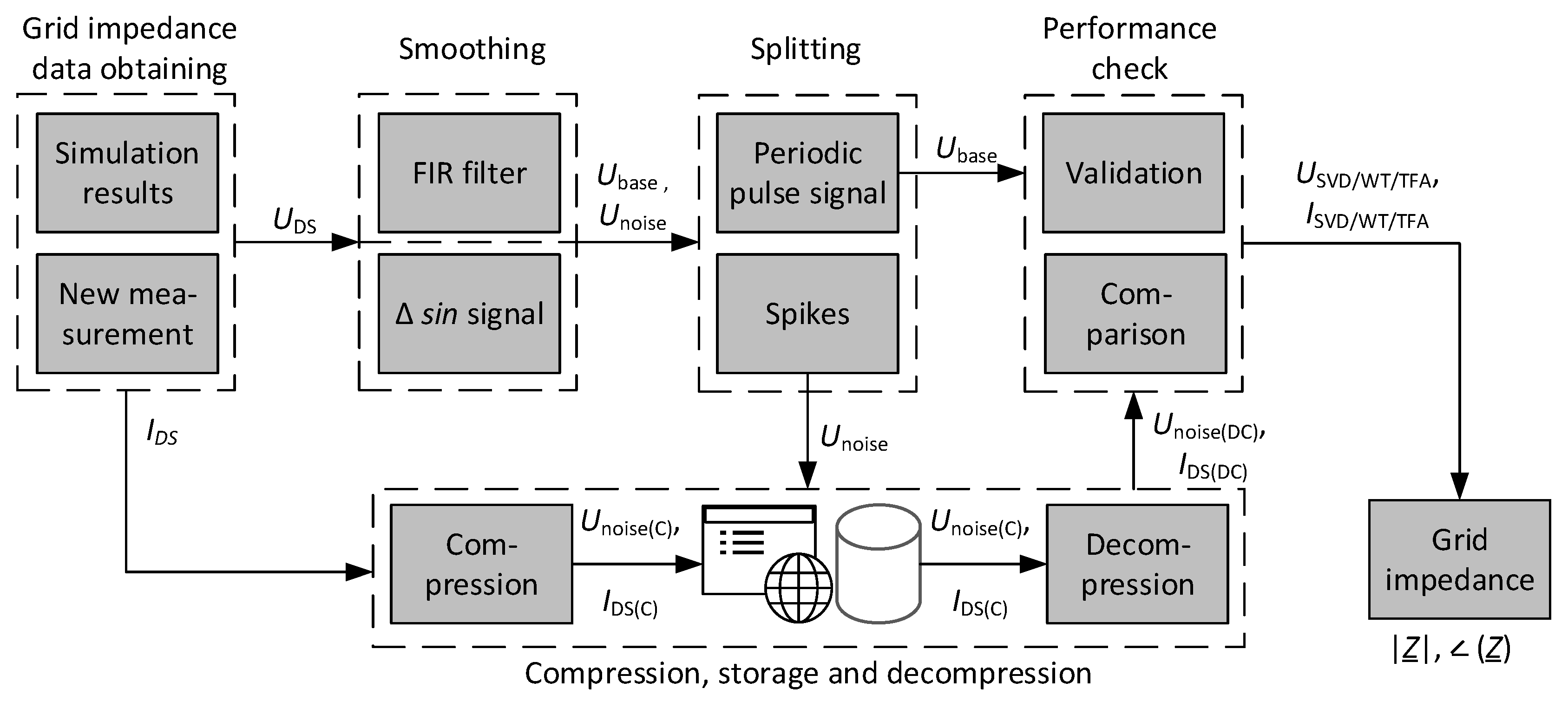
4.1. Novel Approach

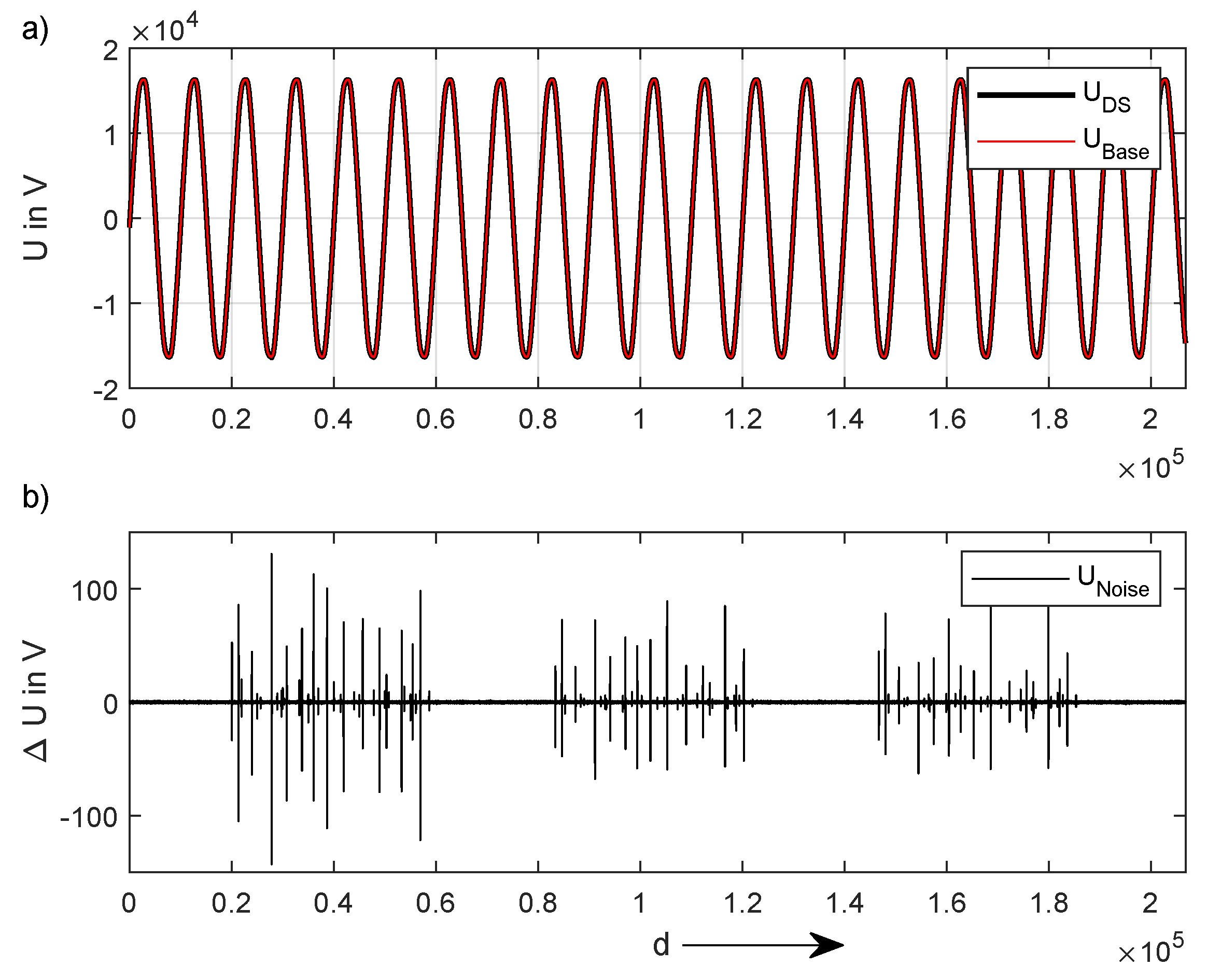
The first step to compress and decompress the impedance data is the generation of the dataset obtained from impedance measurements (Section 2). In a second step, the dataset is smoothed to generate a periodic pulse signal with spikes. For this step, either the moving average filter (FIR filter) method or the $\mathsf{\Delta }sin$-signal method is chosen. The latter method uses the basic function of the voltage output (depending on the measured dataset (7)) to extract the noise of the input function of $U_{\mathrm{DS}}$. The basic function (7) is determined by the impedance evaluation program and approximated by using fitting algorithm toolboxes.

$$\begin{array}{ccc}\hfill U_{\mathrm{base}}& =& \sqrt{2}·11.56\mathrm{kV}·sin\left(2\pi ·48\mathrm{Hz}·t\right)\hfill \end{array}$$

(7)

The result of delta $(U_{\mathrm{base}}-U_{\mathrm{DS}})$ or the FIR-filter output from delta $(U_{\mathrm{FIR}}-U_{\mathrm{DS}})$ extracts the difference, the so-called spikes $U_{\mathrm{noise}},I_{\mathrm{noise}}$, shown in Figure 6. These spikes are challenging to compress and the main reason for the complexity of the developed approach. Typically, existing programs (e.g., smooth from Matlab) smooth out these minimal data swings or spikes directly, thus eliminating the possibility to determine the grid impedance (depending on $U_{\mathrm{DS}}$).

Regarding the current, this procedure can only be carried out with the FIR filter because the I function cannot be readjusted similarly.

Step 3 includes the compression of the dataset. Using different types of lossy compression algorithms, the spikes $U_{\mathrm{noise}}\left(\mathrm{C}\right)$ and the current $I_{\mathrm{DS}}\left(\mathrm{C}\right)$ are converted into a compressed dataset that is stored or saved in online or local data storage systems by their owner (e.g., distribution grid owner, utilities, etc.). After decompression, the recombination of the basic signal and the decompressed spikes is realised (only for the voltage). A validation of the output signal and an automatic performance check, including a comparison between the different compression approaches, ensues. As a result, the generated grid impedance can be compared to the input dataset (and the determined grid impedance) to determine the differences and whether or not the procedure has to be repeated. A flowchart and overview of these steps are shown in Figure 7.

4.2. Key Metrics

Between different compression algorithms, the compared key factors are the processing duration and the errors in combination with compression ratios to achieve an accurate reconstruction result. To ensure a valid comparison of the different types of compression algorithms, different key metrics are used. The compression ratio CR is defined in (8).

$$\begin{array}{cc}\hfill CR& ={\displaystyle \frac{\mathrm{size} \mathrm{of} \mathrm{the} \mathrm{input} \mathrm{dataset} (\mathrm{measured}, \mathrm{uncompressed})}{\mathrm{size} \mathrm{of} \mathrm{the} \mathrm{output} \mathrm{dataset} \left(\mathrm{compressed}\right)}}\hfill \end{array}$$

(8)

Following this definition, values greater than 1 indicate compression and values less than 1 imply expansion. The loss of information will be measured by comparing the reconstructed data matrix $\mathbf{XR}$ (with their rows and columns $n_{\mathrm{row}}·n_{\mathrm{col}}$) with the original data matrix $\mathbf{X}$. The so-called MAE—mean absolute error is defined in (9).

$$\begin{array}{cc}\hfill MAE& ={\displaystyle \frac{1}{n_{\mathrm{row}}·n_{\mathrm{col}}}}\sum _{i=1}^{n_{\mathrm{row}}}\sum _{j=1}^{n_{\mathrm{col}}}\left|\mathbf{X}(i,j)-\mathbf{XR}(i,j)\right|\hfill \end{array}$$

(9)

5. Results

To generate comparable results, all compression approaches are set on a CR round about 4:1. This CR is like a trade-off between the advantages of compression and sufficiently high data fidelity, but randomly chosen for this test case. Although higher CRs are technically possible, this is not the objective of this paper. A comparison of all results for the compression of $U_{\mathrm{Noise}}$ and $I_{\mathrm{DS}}$ is displayed in

Table 1. Compression factor, MAE and processing time of different compression approaches for $U_{\mathrm{noise}}$ and $I_{\mathrm{DS}}$.

Type	CR (U)	MAE (U)	t (U)	CR (I)	MAE (I)	t (I)
SVD	4.1:1	0.36	120 s	4.2:1	0.001	113 s
WT	4.0:1	0.39	8 s	4.0:1	0.002	31 s
TFA	4.2:1	0.29	101 s	4.7:1	0.17	261 s

.

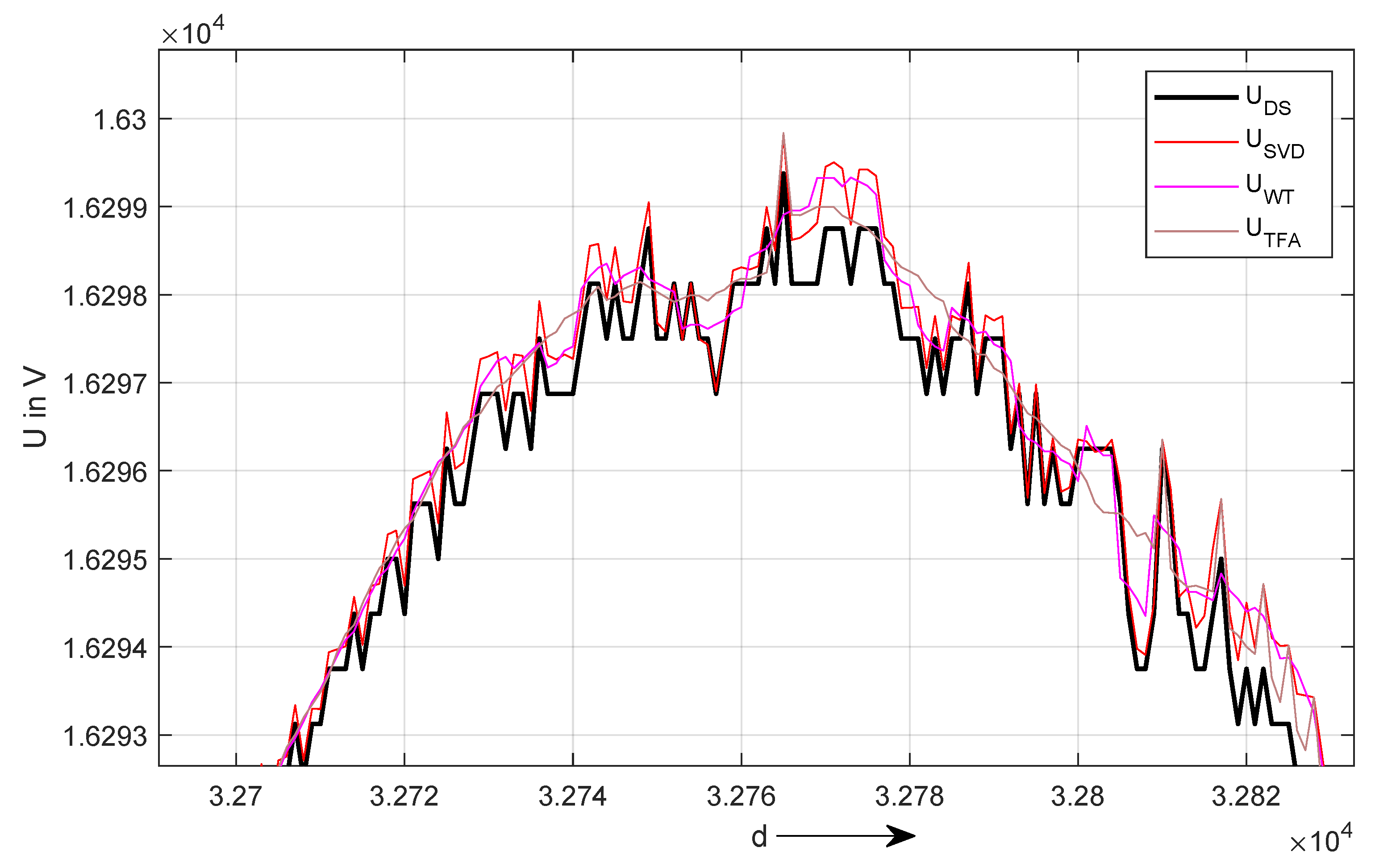
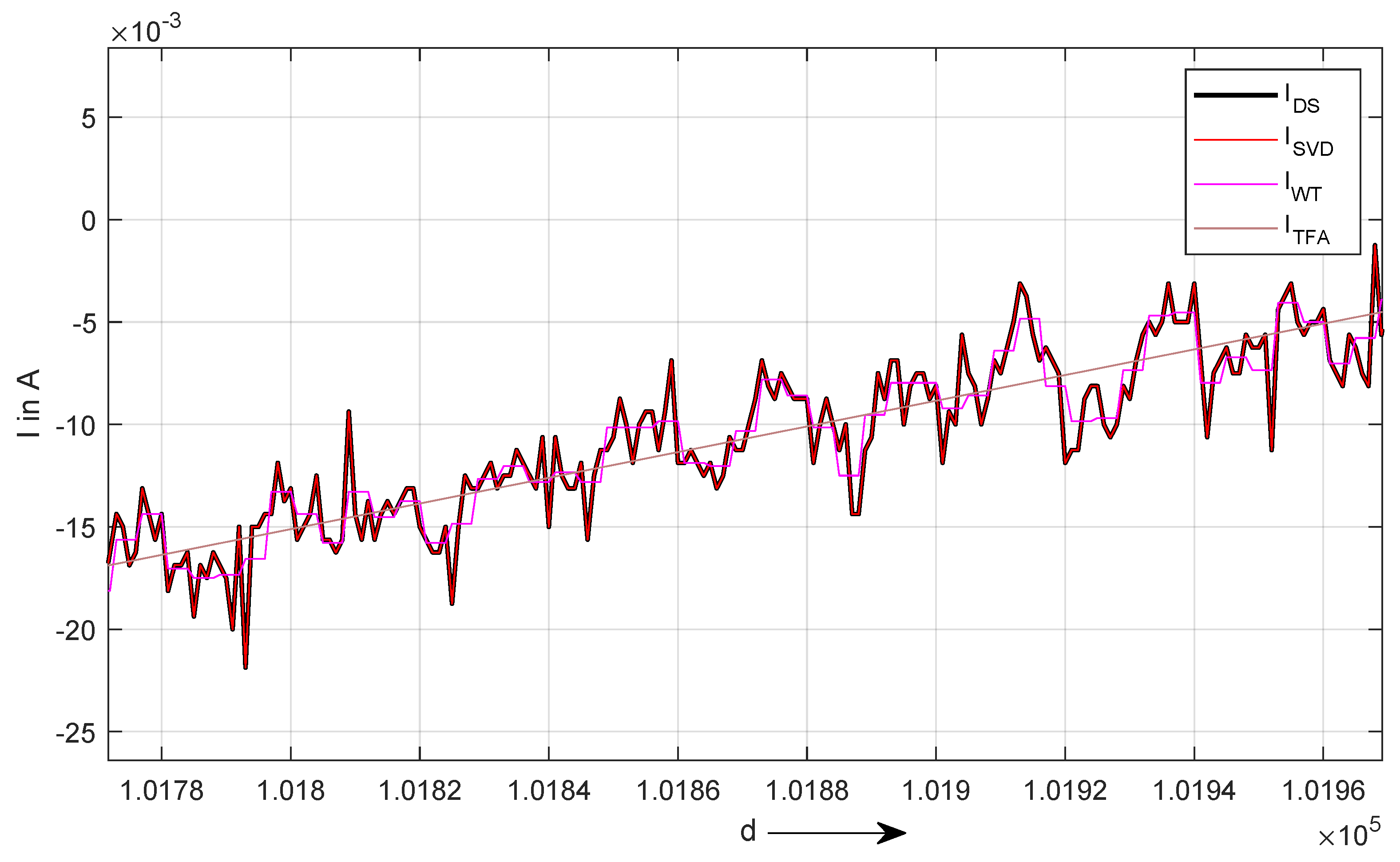
The proposed approaches have been implemented using MATLAB and performed on a PC Intel core i5-3210M processor, 2.50 GHz, with 4 GB of RAM. To illustrate the difference between the approaches, Figure 8 and Figure 9 show the resulting decompression graphs for $U_{\mathrm{Noise}}$ and $I_{\mathrm{DS}}$. In particular, the TFA algorithm does not possess good compression properties, especially when looking at Figure 9. The original curve is simply linearized because of a sluggish (high) threshold (±m$\sigma$), even if the resulting MAE is as good as in the other compression methods.

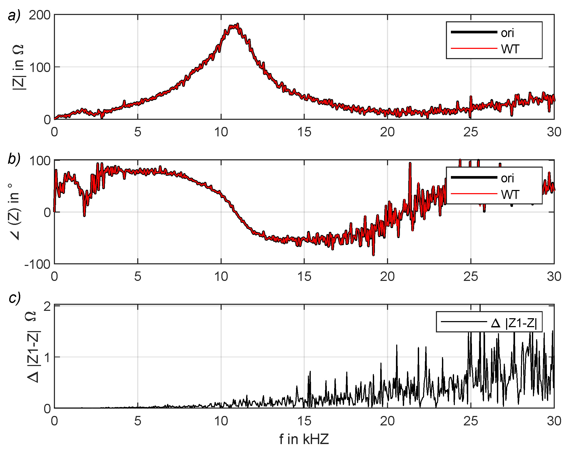
Only the WT and SVD algorithms yield accurate values for the impedance after the recombination of $U_{\mathrm{base}}$ and the decompressed $U_{\mathrm{noise}}\left(\mathrm{DC}\right)$ including the decompressed current $I_{\mathrm{DS}}\left(\mathrm{DC}\right)$. WT shows a particularly good fit of its decompressed impedance values Z to the original values $Z_1$ (Figure 10). Based on (10), Figure 10 shows the absolute impedance $\left|Z\right|$ (a), the impedance angle $\angle \left(Z\right)$ = ${\phi }_{\mathrm{Z}}$ (b), and the absolute deviation $\mathsf{\Delta }\left|Z1-Z\right|$ (c) over the frequency f.

$$\begin{array}{cc}\hfill \underline{Z}& =\left|Z\right|{\phi }_{\mathrm{Z}}\hfill \end{array}$$

(10)

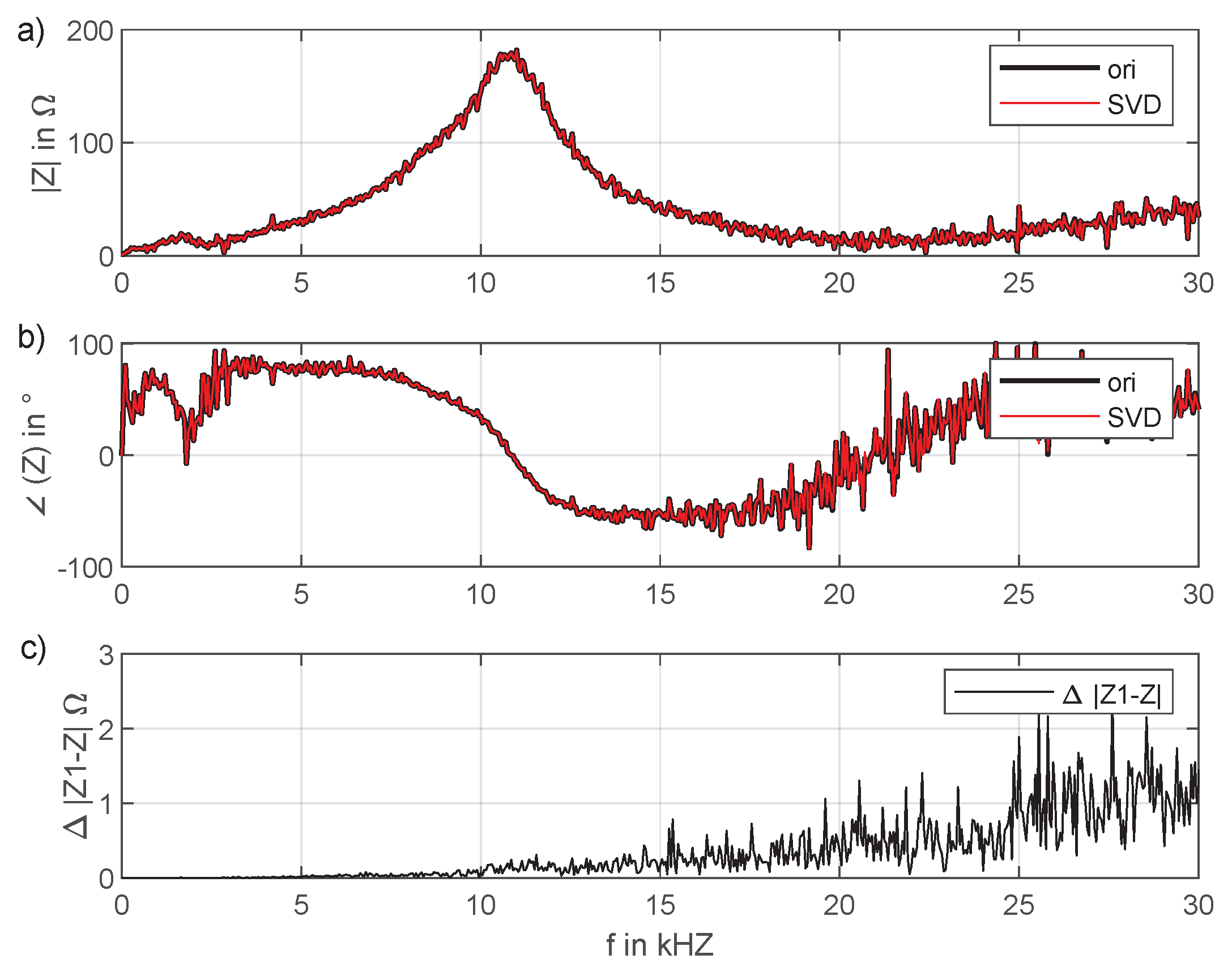
Only for frequencies ≥ 25 kHz do the discrepancies in the WT results increase slightly (≥1%), see Figure 10 (bottom). In comparison see Figure 11, the results obtained by the SVD algorithm deviate from the original dataset by almost 2% for f ≥ 25 kHz. Depending on $I_{\mathrm{DS}}$, the TFA algorithm produces a large deviation of the MAE that leads to the significantly worse results.

Additionally, both the SVD and the TFA algorithms show high processing times $t\left(I\right),t\left(U\right)$ (Table 1). An evaluation of the best fitting technique based on the processing time is only possible to a limited extent. Compression using SVD and WT should be investigated for each data set separately. Conclusively, the TFA algorithm is deemed inadequate to handle the task discussed in this paper or similar tasks.

6. Conclusions

A more detailed understanding of the effects of different voltage and current profiles on the grid impedance requires large amounts of data, especially in the future.

Thus, a very important question is whether or not it is possible to compress data sets from impedance measurements of energy systems by using lossy compression algorithms while maintaining data fidelity. In this paper, the authors show that especially the WT (Wavelet transform) show promising results by reducing the size of the dataset in an efficient way without losing relevant information. The SVD (Singular Value Decomposition) generates almost comparable results, but need much more processing time, referring to the used programming language and computational environment. The presented approach allows of easy and effective data compression with only limited computational resources and, as a result, an increase in the number of measurements that can be stored. It is also conceivable that the presented approach can be applied for efficient online or on-site external server data backup.

While high compression levels are useful in order to reduce the data amount for e.g., utilities, the needed level of data fidelity in the output dataset depends on the targeted application. That is why it is not the objective of this paper to create the best technique and perform on a given dataset. Lossy compression works better when the nature of the compressed data is taken into account (e.g., such as human ear characteristics in MP3). To be able to determine the limits of usability of lossy compression methods, further analyses need to be done. It must be analysed which lossy method generates the best possible outcome i.e., the maximum level of accuracy with the highest suitable compression ratio.

A comparison with lossless compression methods is also interesting. And the authors want to assess if the proposed method is suitable for on-line impedance measurement [4,5].