Abstract
In this work, an effective calculation method of the ion flow field that considers the impact of wind flow and water drops is presented. To be explicit, the nominal electric field is solved by the charge simulation method (CSM) whilst the space charge density is calculated adopting a second order upwind finite volume method. In addition, a method that determines the roughness factor of a conductor surface is used to enhance calculation accuracy. The influence of various properties of the water drops exerting on an ion flow field is analyzed. Eventually, a practical experiment is conducted to verify the calculated result, and the effectiveness and reliability of this method are then proved via comparing calculated and measured results.
1. Introduction
The electromagnetic environment near a high voltage DC (HVDC) transmission line is a primary concern in the electric power system, especially in certain meteorological conditions of fog and rain. In such conditions, the water drops that impinge on the conductor decrease the surface roughness factor and subsequently reduce the onset voltage of corona discharge. In the meantime, the other water drops suspending around the conductor will be charged, and then the ion flow field is affected to a certain degree. Since the corona discharge and the concomitant ion flow field may lead to issues of radiation interference, noise interference and corona loss, investigation of the ion flow field under foggy and rainy weathers, in where the ion flow field is distorted in a more intensive manner, becomes inevitable. Accurate calculation of an ion flow field has the benefit of safe operation and provides a design basis of a transmission line when it goes across areas with greater precipitation and lower temperature.
Methods calculating ion flow field under a transmission line have been developed for decades, and the most frequently used method is the means of solving electric field and space charge distribution separately and iteratively. To find an approximate solution, differences are generally reflected in how the electric field and the space field are calculated. Over the past decades, a considerable amount of the solutions of ion flow fields have been developed. The finite element method (FEM) and method of characteristics (MOC) have been the most frequently adopted in recent years to solve electric field and space charge density, respectively [1,2,3,4,5]. However, FEM has an issue of the accuracy of an electric field near a conductor surface. Additionally, the principle of MOC primarily depends on the Deustch’s assumption that disregards the impact of space charge on the direction of the electric field, and it has been proved inaccurate. Further, certain researches apply the finite volume method (FVM) to solve the current continuity equation for space charge density [6,7,8], which is based on Gauss’ Law and improves calculation accuracy and numerical stability. Also, FVM with unstructured meshing, which possesses second order accuracy and fits for complex geometries, is developed by Z. Long [9]. Moreover, a number of authors [10,11,12,13] calculate the ion flow field using fully coupled upwind FEM to avoid the oscillation that occurs in the process of a space charge solution.
To date, the majority of research focuses on the particle dynamic inside a coupled multi-phase field consisting of electrostatics, gas flow and particle phase. However, the major purpose is to verify the collection efficiency of electrostatics precipitator (ESP) equipment [14,15,16]. Further, in practical application, S Malinowski et al. [17] prepared a laccase sensing layer of electrochemical biosensors using the Corona SPP (Soft Plasma polymerization) technique. Nevertheless, few studies laid emphasis on the ion flow field altered by particle phase in a different perspective, particularly for the HVDC transmission line, which bears resemblance to ESP but still has certain differences in terms of electrode placement, voltage level and particle characteristics. X Bian researched the ion flow field in a corona cage and compared the result with that of an outdoor overhead transmission line. The distribution of space charge density in a coaxial metal cage is measured in [18], the radical space charge density distribution encircling the conductor is analyzed. P.S Maruvada [19] and T Lu [20] calculate the ion flow field considering the impact of wind flow. Y Yi et al. [21] investigates the ion flow field of an HVDC transmission line expressing concern on the influence of Kaolin particles, and the experiment is set up to examine the calculated result. Yet, the impact of water drops, of which the diameters sizing from 1 to 100 m in general rainy and foggy weathers, may differ from that of solid particles. Simultaneously, the influence of wind flow tends to be unnoticeable as the velocity is comparatively low. In contrast with the works mentioned above, in this paper, the influence of both wind flow and water drops are taken into account in the calculation of the ion flow field, by which this method is able to fit in with the actual situation. In addition, this work provides an extended application scenario of plasma in the aspect of high voltage power transmission.
In the calculation of the ion flow field in the presence of water drops, factors that influence calculation accuracy are the selected numerical method and the determination of the roughness factor of the conductor surface. With an aim to improve the calculation accuracy, this work concentrates upon the change of the ion flow field around the transmission line, which is caused by the water drops flowing past the conductor. Along this line of consideration, the ion flow field is calculated through both analytical and numerical methods, and the impact of charged water drops is analyzed. Then, the reduced-scale experiment is set up to validate the calculated result. Meanwhile, by means of comparing the calculated and measured values of ion current density, the roughness factor of the conductor surface is achieved.
2. Methodology
2.1. Governing Equations of Ion Flow Field
In the solution, the ionization layer close to the conductor is neglected. Furthermore, Kaptzov’s assumption [22] is adopted. Specifically speaking, Kaptzov assumes that the electric field on the conductor surface stops growing once corona discharge initializes, this value of the electric field is called onset electric field and is utilized as a boundary condition of the electric field. Equations that govern the ion flow field are described as [1]:
where,
- is the space charge density, C/,
- is the charge density of negative ions, C/;
- is the charge density of water drops, C/;
- b is the mobility of negative ions, ;
- is the total electric field, V/m;
- is the wind velocity vector, m/s;
- is the permittivity of air, .
2.2. Electric Field Calculation
The solution of the electric field is composed of the nominal field and the field generated by the space charges derive from ions and water drops in the calculation domain. Normally, the analytical method possesses higher precision in contrast to the numerical method, such as FVM and the finite difference method (FDM). In this method, CSM is utilized to solve the nominal field [23]. Simulation charges placed in the conductor interior are solved by:
where,
- and are the potential coefficients of the conductor surface and the ground;
- represents the simulation charges, C.
Then, the nominal electric field is hereby solved via superposing the contributions of all the simulation charges. Additionally, the total electric field can be attained when the space charge distributions of ions and water drops are known. The expression is shown as below:
where,
- is the nominal electric field on conductor surface, V/m;
- , and are the distances between observation points and simulation charges, m;
- , and are the distances between observation points and image charges, m;
- s is the area of cell, .
2.3. Space Charge Density
The space charge density spans charges of ions and water drops, with respect to the ion charges, and the second order upwind finite volume method (UFVM) is utilized in which the gradient of the space charge density is solved and applied to obtain the space charge density on the control volume edges. In this context, the calculated charge distribution precision is substantially promoted compared with the traditional FVM method that regards charge density as evenly distributed. Generally, there should be an initial value of the charge density on the conductor surface, the empirical formula presented in [24] is used:
where,
- is the initial value of conductor surface charge density, C/;
- is the electric field on the ground under conductor, V/m;
- r is the radius of conductor, m;
- is the onset voltage of conductor, V;
- is the applied voltage, V;
- is the height of the conductor above the ground, m.
The following equation can be achieved according to Equation (1):
The integral form is:
where l is the boundary of the control volume.
Equation (6) is subsequently converted into a system of linear equations in accordance with the sketch map of control volume in Figure 1:
where,
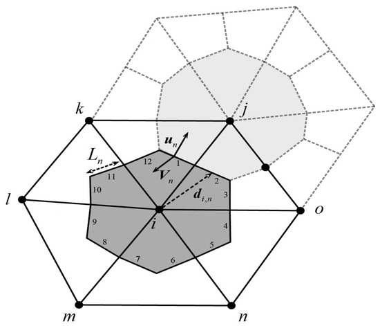
Figure 1.
Control volume.
- n is the serial number of cell edges;
- and are the normal vectors of the electric field and wind speed on cell edges;
- are the lengths of cell edges, m.
Charge densities of control volumes are then attained. The charge density on the mutual edge of two adjacent control volumes is expressed as below based on Taylor series expansion:
where,
- is the normal vector from the node to the corresponding adjacent cell edge;
- and are the gradients of the upwind node, which is solved by:
- , are the increments in the x and y direction, m;
- and are the rates of change of the charge densities of the ith node;
- is the charge density of adjacent cell, C/.
For the charge density of water drops, the medium volume diameter (MVD) of the water drops used in this work is above 50 s. Thus, only the field charging mode is considered during the charging process. As well, certain assumptions are proposed:
- Water drops are evenly distributed and their diameters are presented by MVD;
- Collisions between water drops are ignored;
- The shape of water drops remains spherical.
Once water drops enter the calculation domain, the charging process is initialized. Charge quantity of a single water drop is characterized by [15]:
is the saturation charge of a single water drop, which is described as:
where,
- is the relative permittivity of water, F/m;
- is the diameter of water drop, m;
- is the time coefficient that stands for the amount of time for the water drop to be half saturated:
As illustrated in Figure 2, the charge saturation rate climbs to a high level around 95%, and then approaches approximately constant for a long span of time. Thus, the charges of water drops are assumed to be invariant, and because the spray nozzle is positioned 40 cm away from the entrance of calculation domain, charges of water drops reach a stable level before entering the calculation domain.
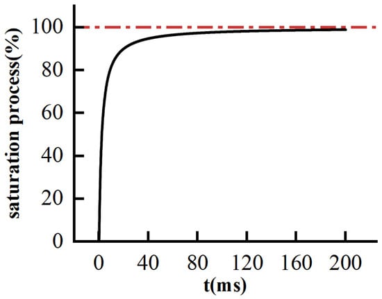
Figure 2.
Charging rate of single water drop.
The acceleration of a charged water drop in the ion flow field is calculated by the equation below [25]:
where,
- p is the dipole moment of water drop;
- is the volume of water drop, ;
- can be obtained when the size and volume fraction of water drop is known:
The volume fraction is achievable by the following equation:
where,
- Q is the water flow rate of the water spray nozzle, L/s;
- is the sectional area, .
Obviously, the acceleration is independent of the dimension of water drop and the electric field. The variation of is solved by means of substituting the electric field addressed earlier, the result indicates that the acceleration of the water drop of macron grad caused by electric force is less than −0.2 at the position where it is 5 cm away from the conductor surface, it decreases significantly along with approaching the boundary of the calculation domain. Moreover, the trajectories of water drops are assumed to be compatible with the wind flow [26]. Because the ratio of conductor diameter and the calculation domain, which is 2%, the impact of the motion fluctuation of the charged water drops stemming from the flow turbulence on the electric field and the space charge density is negligible, especially for the charge density on the ground level.
2.4. Iteration Terminal Criterion
The terminal criterion are defined to be the differences of E and of two successive iterations:
where,
- and are the terminal criterion;
- is the electric field of conductor surface, V/m;
- and are the space charge densities of two adjacent iterations of the ith cell, C/.
The charge density on the conductor surface is modified in each iteration till the terminal criterion are reached:
where and are the previous and current charge densities on the conductor surface, respectively, C/.
The detailed process is shown below in Figure 3.
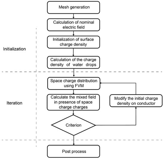
Figure 3.
Flow chart of the ion flow field calculation.
In regards to the onset electric field intensity [27], the empirical expression is shown in Equation (19):
The roughness factor m dominantly controls the onset voltage as the adhesion of water drops intensifies the local electric field distortion on the conductor surface. Therefore, determination of the roughness factor is crucial in the ion flow field calculation. In this work, the roughness factor is attained through comparing the calculated and measured ion flow current. The detailed process is shown in Figure 4.
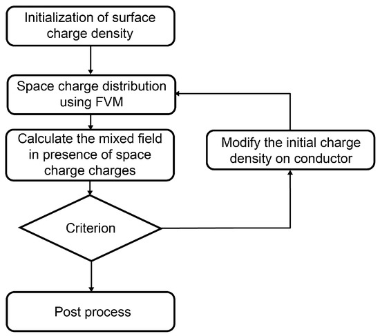
Figure 4.
Flow chart of roughness factor determination.
3. Validation
The experiment was conducted in a tunnel constructed by transparent acrylic boards, as illustrated in Figure 5. The cross-section is 500 mm square and the length of the tunnel is 900 mm.
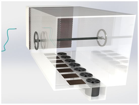
Figure 5.
Schematic diagram of experiment setup.
The stranded conductor goes across the tunnel transversely and is hung at the center points of two opposite sides. The radius of the conductor is 10 mm in this experiment. Regarding the measurement of electric field and ion flow current, seven field mills and seven 100 × 80 mm Wilson plates are flush-mounted beneath the conductor in parallel. Signals of the Wilson plates were collected by scope corder DL-850. The voltage supply is an adjustable DC voltage generator. Wind flow of 0–10 m/s was provided by a fan and passed through a flow equalizing plate to reduce fluctuation. The wind velocity was measured by a high precision digital anemometer (AS-8336). A spray pump was used to generate water drops, and two nozzles with different diameters were adopted to control the MVD of water drops. All of these are illustrated in Figure 6.
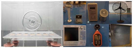
Figure 6.
Experimental installation.
The experiment was implemented in an enclosed phytotron, where the temperature was set to be 15 C throughout the whole experimentation. It is worth noting that the humidity in the phytotron was insured to be saturated in order to eliminate the influence of changing humidity during the spray process.
4. Discussion
The wind flow velocity and the parameters of water drops were set to be the variables with the goal of investigating their influences on the electric field and ion flow current beneath the conductor. In this experiment, water drops with MVDs of 58 and 92 m were adopted while the wind velocity was fixed to 0, 5, and 10 m/s, respectively. Concurrently, the influence of diverse volume fraction rates in the circumstance of the 58 m diameter water drops was investigated.
The relevant calculated and experimental results are demonstrated in Figure 7. The results reveal that the electric field is influenced by the charged water drops together with the wind flow velocity to a slight extent. However, shifts of the curves remain visible owing to the increment of the charge quantity of water drops and the wind flow velocity. It proves that the electric field is primarily dominated by the energized electrode rather than the space charge density.
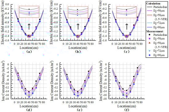
Figure 7.
(a–c) Electric field intensity of 0, 5 and 10 m/s wind velocity; (d–f) ion current density of 0, 5 and 10 m/s wind velocity.
With regard to the ion current density, the influence caused by the charged water drops becomes more apparent, because the ion current density is purely a reflection of the space charge density. Additionally, the growth of ion current density mainly reflects the change of the charge quantity of the water drop because the variation of the electric field is moderate, which leads to a basically unchanged charge quantity of ions. Furthermore, the influence of the rise of wind flow velocity tends to be more discernible when the velocity reaches 10 m/s. In addition, the assumption that regards the charge quantity of water drops as uniformly distributed in the calculation domain is supported, since there is nearly no difference observed between the symmetric measurement points with respect to the midpoint. As a consequence, such result manifests that the influence of charged water drops is decided by the total charge amount they are holding.
The ion flow field under the wind flow velocity of 15m/s is calculated as a limiting case, so as to evaluate the influence of strong wind that is unable to achieve in the experiment. However, this situation is calculated and the result is demonstrated in Figure 8. Meanwhile, the simulated result of the space charge density is shown in Figure 9. They both manifest that the degree of the shift caused by wind flow arises, especially the ion current density and the space charge density. As the experiment is set in a tunnel rather than a practical overhead transmission line, it is predictable that the ion flow field will move a large distance because of the attenuated electric field on the ground level.
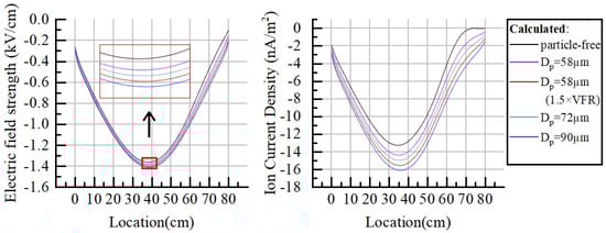
Figure 8.
Calculated electric field intensity and ion current density under 15 m/s wind velocity.
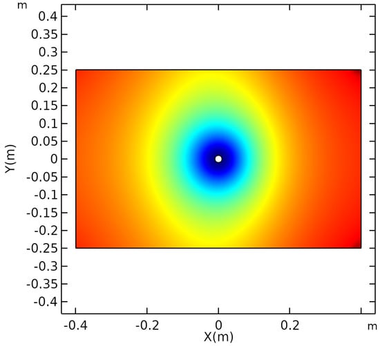
Figure 9.
Simulation result of the space charge density under 15 m/s wind velocity.
As the impact of charged water drops and wind flow velocity on the ion flow field is considerable, accurate and effective calculation facilitates the evaluation of the electromagnetic environment near transmission lines under various weather conditions. Accordingly, site selections of the infrastructures along the transmission line corridor could refer to the distribution of the ion flow field, for instance, railway, communication facility and residential area. In the meantime, conductor parameters, for example, the diameter and the number of strands, can be optimized according to the roughness factor determination method.
5. Conclusions
In summary, this paper firstly proposed the calculation method of an ion flow field that considers the influence of water drops and wind velocity. Sequentially, an experiment is designed and conducted to examine the calculated result. The comparison of numerically calculated and measured data agrees well, which proves the presented method. Secondly, determination of the roughness factor of the conductor surface is presented to improve the calculation accuracy in the situation that the conductor is adhered to by water drops. Furthermore, it provides an approach to predict the surface condition by means of ion current density measurement. As a result, it is clarified that the ion flow field, especially the ion flow current, is affected to a certain extent under rainy and foggy weather. Therefore, environmental factors of water drops and wind flow should be taken into full consideration in the design phase of a transmission line, for instance, to adopt a bundle conductor for the purpose of decreasing the electric field on a conductor surface, by which the probability of corona discharge will reduce accordingly.
Author Contributions
Conceptualization, Z.L. and X.Z.; Methodology, Z.L.; Software, Z.L.; Validation, Z.L.; Writing-Original Draft Preparation, Z.L.; Writing-Review & Editing, Z.L. and X.Z.; Supervision, X.Z.; Project Administration, X.Z. All authors have read and agreed to the published version of the manuscript.
Funding
This research received no external funding
Conflicts of Interest
The authors declare no conflict of interest.
References
- Janischewskyj, W.; Gela, G. Finite element solution for electric fields of coronating DC transmission lines. IEEE Trans. Power Appar. Syst. 1979, PAS-98, 1000–1012. [Google Scholar] [CrossRef]
- Xiao, F.; Zhang, B.; Mo, J.; He, J. Calculation of 3-D ion-flow field at the crossing of HVdc transmission lines by method of characteristics. IEEE Trans. Power Deliv. 2017, 33, 1611–1619. [Google Scholar] [CrossRef]
- Bian, X.; Yu, D.; Meng, X.; MacAlpine, M.; Wang, L.; Guan, Z.; Yao, W.; Zhao, S. Corona-generated space charge effects on electric field distribution for an indoor corona cage and a monopolar test line. IEEE Trans. Dielectr. Electr. Insul. 2011, 18, 1767–1778. [Google Scholar] [CrossRef]
- Al-Hamouz, Z.M. Corona power loss, electric field, and current density profiles in bundled horizontal and vertical bipolar conductors. IEEE Trans. Ind. Appl. 2002, 38, 1182–1189. [Google Scholar] [CrossRef]
- Li, W.; Zhang, B.; He, J.; Zeng, R.; Chen, S. Ion flow field calculation of multi-circuit DC transmission lines. In Proceedings of the 2008 International Conference on High Voltage Engineering and Application, Chongqing, China, 9–12 November 2008; pp. 16–19. [Google Scholar]
- Yin, H.; Zhang, B.; He, J.; Zeng, R.; Li, R. Time-domain finite volume method for ion-flow field analysis of bipolar high-voltage direct current transmission lines. IET Gener. Transm. Distrib. 2012, 6, 785–791. [Google Scholar] [CrossRef]
- Levin, P.L.; Hoburg, J.F. Donor cell-finite element descriptions of wire-duct precipitator fields, charges, and efficiencies. IEEE Trans. Ind. Appl. 1990, 26, 662–670. [Google Scholar] [CrossRef]
- Meroth, A.; Gerber, T.; Munz, C.; Levin, P.; Schwab, A. Numerical solution of nonstationary charge coupled problems. J. Electrost. 1999, 45, 177–198. [Google Scholar] [CrossRef]
- Long, Z.; Yao, Q.; Song, Q.; Li, S. A second-order accurate finite volume method for the computation of electrical conditions inside a wire-plate electrostatic precipitator on unstructured meshes. J. Electrost. 2009, 67, 597–604. [Google Scholar] [CrossRef]
- Huang, G.; Ruan, J.; Du, Z.; Zhao, C. Highly stable upwind FEM for solving ionized field of HVDC transmission line. IEEE Trans. Magn. 2012, 48, 719–722. [Google Scholar] [CrossRef]
- Zhou, X.; Lu, T.; Cui, X.; Zhen, Y.; Liu, G. Simulation of ion-flow field using fully coupled upwind finite-element method. IEEE Trans. Power Deliv. 2012, 27, 1574–1582. [Google Scholar] [CrossRef]
- Liu, J.; Zou, J.; Tian, J.; Yuan, J. Analysis of electric field, ion flow density, and corona loss of same-tower double-circuit HVDC lines using improved FEM. IEEE Trans. Power Deliv. 2008, 24, 482–483. [Google Scholar]
- Lu, T.; Feng, H.; Zhao, Z.; Cui, X. Analysis of the electric field and ion current density under ultra high-voltage direct-current transmission lines based on finite element method. IEEE Trans. Magn. 2007, 43, 1221–1224. [Google Scholar] [CrossRef]
- Adamiak, K.; Atten, P. Numerical simulation of the 2-D gas flow modified by the action of charged fine particles in a single-wire ESP. IEEE Trans. Dielectr. Electr. Insul. 2009, 16, 608–614. [Google Scholar] [CrossRef]
- Skodras, G.; Kaldis, S.; Sofialidis, D.; Faltsi, O.; Grammelis, P.; Sakellaropoulos, G. Particulate removal via electrostatic precipitators—CFD simulation. Fuel Process. Technol. 2006, 87, 623–631. [Google Scholar] [CrossRef]
- Zhuang, Y.; Kim, Y.J.; Lee, T.G.; Biswas, P. Experimental and theoretical studies of ultra-fine particle behavior in electrostatic precipitators. J. Electrost. 2000, 48, 245–260. [Google Scholar] [CrossRef]
- Malinowski, S.; Wardak, C.; Jaroszyńska-Wolińska, J.; Herbert, P.A.F.; Pietrzak, K. New electrochemical laccase-based biosensor for dihydroxybenzene isomers determination in real water samples. J. Water Process. Eng. 2020, 34, 101150. [Google Scholar] [CrossRef]
- Zhou, X.; Cui, X.; Lu, T.; Fang, C.; Zhen, Y. Spatial distribution of ion current around HVDC bundle conductors. IEEE Trans. Power Deliv. 2011, 27, 380–390. [Google Scholar] [CrossRef]
- Maruvada, P.S. Influence of wind on the electric field and ion current environment of HVDC transmission lines. IEEE Trans. Power Deliv. 2014, 29, 2561–2569. [Google Scholar] [CrossRef]
- Lu, T.; Feng, H.; Cui, X.; Zhao, Z.; Li, L. Analysis of the ionized field under HVDC transmission lines in the presence of wind based on upstream finite element method. IEEE Trans. Magn. 2010, 46, 2939–2942. [Google Scholar] [CrossRef]
- Yi, Y.; Zhang, C.; Chen, Z.; Wang, L. Influence of aerosols on the ion-flow field under high-voltage direct current transmission lines. IET Gener. Trans. Distrib. 2016, 10, 1479–1485. [Google Scholar] [CrossRef]
- Kaptzov, N. Electricheskie Invelentiia v Gazakh I Vakuumme; OGIZ: Moscow, Russia, 1947. [Google Scholar]
- Abdel-Salam, M.; Abdel-Aziz, E. A charge simulation based method for calculating corona loss on AC power transmission lines. J. Phys. Appl. Phys. 1994, 27, 2570. [Google Scholar] [CrossRef]
- Abdel-Salam, M.; Al-Hamouz, Z. A finite-element analysis of bipolar ionized field. IEEE Trans. Ind. Appl. 1995, 31, 477–483. [Google Scholar] [CrossRef]
- Yin, F.; Farzaneh, M.; Jiang, X. Influence of AC electric field on conductor icing. IEEE Trans. Dielectr. Electr. Insul. 2016, 23, 2134–2144. [Google Scholar] [CrossRef]
- Fu, P. Modelling and Simulation of the Ice Accretion Process on Fixed or Rotating Cylindrical Objects by the Boundary Element Method (Modélisation et Simulation des Accrétions de Glace Atmosphérique sur des Objets Cylindriques Fixes et Tournants par la Méthode des Éléments Finis de Frontière); Université du Québec à Chicoutimi: Chicoutimi, QC, Canada, 2004. [Google Scholar]
- Peek, F.W. Dielectric Phenomena in High Voltage Engineering; McGraw-Hill Book Company: New York, NY, USA, 1920. [Google Scholar]
© 2020 by the authors. Licensee MDPI, Basel, Switzerland. This article is an open access article distributed under the terms and conditions of the Creative Commons Attribution (CC BY) license (http://creativecommons.org/licenses/by/4.0/).