A Novel Maximum Power Point Tracking Control Strategy for the Building Integrated Photovoltaic System

Abstract

Thin-film photovoltaic technology has begun to be applied in building-integrated photovoltaics (BIPVs), and it is believed that thin-film photovoltaic technology has potential in building-integrated photovoltaic applications. In this paper, a hybrid approach was investigated which combined the maximum power point tracking (MPPT) algorithm of three-stage variable step size with continuous conduction mode (CCM)/discontinuous current mode (DCM). The research contents of this paper include the principle analysis of the maximum power point tracking algorithm, the design of the sampling period, and the design of a double closed-loop control system and correction factor. A system model was built in MATLAB/Simulink, and a comparative simulation was carried out to compare the performance of the proposed method with some traditional methods. The simulation results show that the proposed approach has the ability to fast-track and make the system run stably. Furthermore, it can make the system respond quickly to environmental changes. An experimental platform was built, and the experimental results validated and confirmed the advantages of the proposed method.

1. Introduction

1.1. Background and Motivation

Building-integrated photovoltaics (BIPVs) are a promising technology to integrate photovoltaic power generation modules and buildings [1]. It is an economical way to utilize renewable energy and could play an important role in meeting the world’s increasing power demand, reducing the consumption of fossil fuels, and protecting the environment [2]. Photovoltaic modules are usually installed on the surface of a protective structure around the building to provide power, while also serving as a functional part of building structure [3,4]. The products can be widely used in sunshades, curtain walls, roofs, doors, and windows. In addition to meeting the requirements of conventional lighting and architectural aesthetics, BIPVs can provide electricity in a clean and environment-friendly way. BIPVs do not occupy extra land, and they reduce the cost of power transmission and energy consumption, saving on the support structure and reducing the overall cost of the building [5,6]. Therefore, the efficiency of the power generation system is high, and the overall cost can be reduced. At present, many countries in the world are trying to reduce the manufacturing cost and improve the power generation efficiency of BIPVs, by improving the manufacturing techniques and expanding the market size [7,8].

Compared with a silicon module, thin-film photovoltaic modules, as the generation units in a BIPV system, have the advantages of electrical characteristics such as high voltage output and good response to weak light. Moreover, the cell structure of a thin-film module is different from a silicon module in that there is no hot spot. Therefore, when partial shading occurs, the power reduction of a thin-film module is much smaller than that of a silicon module. They also have other advantages, such as low production cost, controllable transparency, and energy conservation when used as building materials. Therefore, thin-film photovoltaic technology is the most commonly preferred technology for BIPVs [9].

Unlike traditional photovoltaic power plants, the operating environment of thin-film modules in BIPVs is complex. For example, as a part of the building, the modules are usually not installed at the optimal elevation angle, and these modules could be subjected to sudden changes of light intensity due to shadows cast by clouds, other architecture, people, vehicles, and so on. These problems can cause power loss. In this regard, research into maximum power point tracking (MPPT) becomes crucial [10,11,12].

1.2. Problems and Solution

In the literature, there are many reported control strategies for MPPT. Generally, there are three perturbing methods: the current perturbation method, the duty cycle perturbation method, and the voltage perturbation method. The current perturbation method has low control accuracy and large oscillations around the maximum power point, so it is not common either in theoretical research or engineering applications. The duty cycle perturbation method (also called the perturbation-and-observation method) has been widely studied [13]. However, power oscillations exist near the maximum power point. The perturbation value affects the tracking speed and the oscillation amplitude [14]. The voltage perturbation method (also known as the hill-climbing method) is also commonly used in engineering applications. The key of this method is the closed-loop control of the DC-DC converter. In terms of the control effect or control accuracy, the voltage perturbation method performs better than the former two methods [15,16].

There are many control strategies based on the voltage perturbation method to achieve the maximum power point. Among these control strategies, the most commonly used method is the use of traditional proportion integral differential (PID) controllers because they are simple and easy to implement [17,18]. Usually, most of the PID controllers are designed under a continuous conduction mode (CCM) condition; however, when the environment changes rapidly, the DC-DC converter may work in discontinuous conduction mode (DCM) [19]. The PID controllers designed for CCM cannot be employed in DCM directly; otherwise, the performance of the power generation is reduced. The fuzzy control strategy is simple in design and easy to understand, and it has strong robustness. However, the simple fuzzy processing of information can reduce the control accuracy and dynamic performance of the system [20,21]. The sliding mode control strategy is independent of the control object model, and its system response is fast. However, due to the existence of a sliding surface, there is chattering near the control target (i.e., the maximum power point), and this behavior affects the stability of the system [22]. The artificial neural network control strategy has self-learning and self-adaptive ability, but the algorithm is complex and difficult to realize [23].

In order to address the issues of the above controllers, based on the two-stage variable step size method (improved traditional hill-climbing algorithm), this paper proposes an MPPT algorithm called the three-stage variable step size (3SVSS) method. According to the inherent characteristics of the boost converter, an appropriate selection method of the sampling period is introduced that reduces the system power loss. Based on the traditional double closed-loop (DCL) controllers in CCM and DCM, this paper proposes a CCM/DCM hybrid control strategy where two correction factors are introduced. With the proposed hybrid control strategy, the control accuracy of the system is not reduced when the irradiance changes continuously, especially in an environment with weak light [24,25]. The control strategy proposed in this paper was verified by simulation and experimental work, and the proposed method was also compared to other methods in order to confirm its advantages.

2. Methodology

2.1. Characteristics of the Thin-Film Photovoltaic Modules

In Jain’s work [26], the mathematical equation of the thin-film photovoltaic module is expressed as:

$$I_{pv}=n_p{I}_L-n_p{I}_0\left\{\exp \left[\frac{q(V_{pv}+I_{pv}{R}_s)}{AKT{n}_s}\right]-1\right\}-\frac{V_{pv}+I_{pv}{R}_s}{R_{sh}}$$

(1)

where n_pI_L is the photocurrent; n_pI₀ is the reverse saturation current; q is the electron charge; K is the Boltzmann constant; T is the absolute temperature; A is the diode factor; R_s is the series resistance; and R_sh is the parallel resistance. Its equivalent circuit is shown in Figure 1.

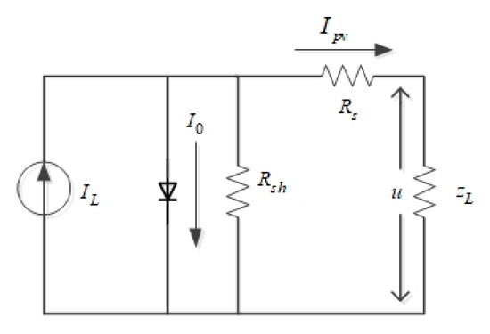
Figure 1. Physical model of the photovoltaic cell.

In engineering applications, considering some specific factors, the two-point method and its improved method are generally used to simplify Equation (1) to a certain extent. That is, parallel resistance is very large, so the part with 1/R_sh can be neglected. Since the series resistance is generally much smaller than the forward-conducting resistance of the diode, the photocurrent is assumed to be equal to the short-circuit current. Then the voltage and current in the open-circuit state and the maximum power point state are substituted into Equation (1) to obtain an approximated model.

$$I_{pv}=I_{sc}\left\{1-C_1\left[\exp (\frac{V_{pv}-dv}{C_2{V}_{oc}})-1\right]\right\}+di$$

(2)

$$C_1=\left(1-\frac{I_{mpp}}{I_{sc}}\right)\exp \left(\frac{V_{pv}-dv}{C_2{V}_{oc}}\right)$$

(3)

$$C_2=\left(\frac{V_{mpp}}{V_{oc}}-1\right)\ln \left(1-\frac{I_{mpp}}{I_{sc}}\right)$$

(4)

$$di=a\frac{S}{S_{ref}}dt+\left(\frac{S}{S_{ref}-1}-1\right)I_{sc}$$

(5)

$$dv=-bdt-R_{s}di$$

(6)

$$dt=T-T_{ref}$$

(7)

In Equations (5)–(7), S_ref = 1000 W/m², a is the current temperature coefficient, and b is the voltage temperature coefficient.

According to Equations (2)–(7), the P-V and I-V curves under different light intensities were obtained, as shown in Figure 2.

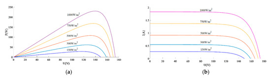
Figure 2. Simulated P-V and I-V curves under different illumination conditions: (a) P-V curves; (b) I-V curves.

2.2. Proposed MPPT Algorithm

As shown in Figure 2, the different illumination intensities hardly affected the shift of the maximum power point. The working temperature generally changed slightly; hence, its effect was not considered in this paper. The maximum power point roughly corresponded to 75% of the open-circuit voltage of the module. In the proposed MPPT algorithm, there are three stages. According to Figure 3, in stage 1, the output voltage of the module is controlled to 75% of the open-circuit voltage without detecting the voltage and current of the module. The following two stages, when approaching the maximum power point, are determination of the disturbing direction and step size by comparing with a smaller set value; hence, the step sizes are smaller than one of the traditional two-stage variable step-size control strategies. The flow chart of the proposed algorithm is shown in Figure 4. The power was calculated using the sampled voltage and current. The change in direction of the voltage was determined by comparing the voltage change with a set value.

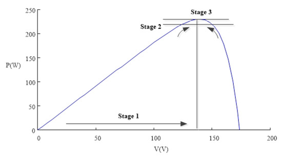
Figure 3. Schematic diagram of the three-stage variable step size.

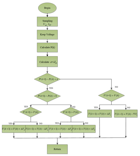
Figure 4. Flow chart of the three-stage variable step size (3SVSS) algorithm.

2.3. Proposed Control Strategy

The DCL control system is shown in Figure 5 as the boost converter works in CCM mode; that is, the output of the voltage loop is the input of the current loop, which is used to generate the pulse width modulation (PWM) signal.

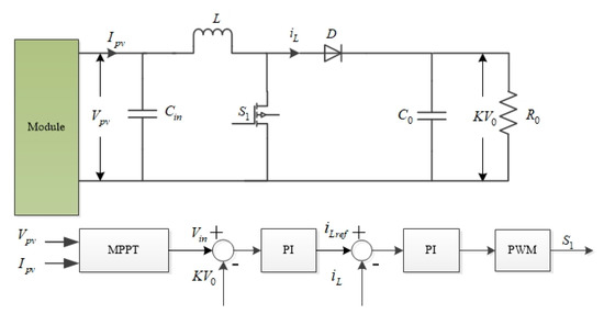
Figure 5. Double closed-loop (DCL) control in the continuous conduction mode (CCM) schematic diagram.

The state–space average modeling of the equivalent circuit of the boost converter is given by:

$$L\frac{d\overline{i_L}}{dt}=V_{in}-V_0+d{V}_0$$

(8)

$$C_0\frac{d\overline{V}}{dt}=(1-d){\overline{i}}_L-\frac{\overline{V}}{R_0}$$

(9)

where d is duty cycle of the switch. The small-signal model of the boost converter is:

$${\overline{V}}_{in}=V_{in}+\stackrel{\wedge }{V_{in}},{\overline{V}}_0=V_0+\stackrel{\wedge }{V_0},d=D+\stackrel{\wedge }{d}$$

(10)

Substituting Equation (10) into Equations (9) and (8) results in:

$$L\frac{d\stackrel{\wedge }{i}}{dt}=\stackrel{\wedge }{V_{in}}-(1-d)\stackrel{\wedge }{V_0}+V_0\stackrel{\wedge }{d}$$

(11)

$$C_0\frac{d\stackrel{\wedge }{V_0}}{dt}=(1-d)\stackrel{\wedge }{i}-\frac{\stackrel{\wedge }{V_0}}{R_0}-\overline{i_L}\stackrel{\wedge }{d}$$

(12)

The open-loop transfer function of the voltage control loop is derived as:

$$G_v(s)=\frac{V_0(s)}{i_{ref}(s)}=\frac{V_{in}-L{I}_{L}s}{K{V}_0(\frac{1}{R_0}+C_{0}s)}$$

(13)

The open-loop transfer function of the current control loop is derived and expressed by Equation (14):

$$G_i(s)=\frac{i_L(s)}{d(s)}=\frac{K{V}_0(\frac{2}{R_0}+C_{0}s)}{L{C}_0{s}^2+\frac{L}{R_0}s+\frac{V_{in}}{I_L{R}_0}}$$

(14)

When the irradiance decreases dramatically or the load increases abruptly, it is likely that the boost converter works in the DCM. The control mechanism in the DCM is different from that in the CCM because of different state–space average models and transfer functions. In order to achieve seamless transition between the two modes, a correction factor is introduced into the system. When the converter is working in CCM, the correction factor is 1, and it has no effect on the system. When the converter is working in DCM, the correction factor can compensate for the output of the CCM feedback. Therefore, the corresponding controller can be modified accordingly. As shown in Figure 6, based on the traditional closed-loop control, the correction factors α_DCM(z) and β_DCM(z) are introduced into the voltage loop and the current loop, respectively, which leads to the proposed CCM/DCM hybrid control. With this control strategy, the boost converter can be regarded as a hybrid automata model. This model includes the continuous process (CP) and the discrete process (DP). According to the continuous state signals of CP, that is the inductor current and output voltage, DP can control the transition of the discrete state as a finite state machine.

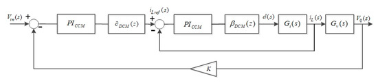
Figure 6. Block diagram of the proposed controller.

The correction factors can be calculated as follows. When the boost converter works in DCM, the state–space average model of the equivalent circuit of the boost converter is given by:

$$\overline{i_L}=\frac{i_{\max }}{2}(d_1+d_2)$$

(15)

$$d_1+d_2<1$$

(16)

$$i_{\max }=\frac{V_{in}}{L}{d}_1{T}_s$$

(17)

$$d_2=\frac{2L{\stackrel{-}{i}}_L}{d_1{T}_s{V}_{in}}-d_1$$

(18)

$$L\frac{d\overline{i_L}}{dt}=\frac{2L\overline{i_L}}{d{T}_s}(\frac{V_{in}-V_0}{V_{in}})+d_1{V}_0$$

(19)

The voltage ratio M in DCM is:

$$M=\frac{V_0}{V_{in}}=\frac{1+\sqrt{1+4d_2{}^2/K_0}}{2}$$

(20)

where K₀ = 2L/R₀T_s, T_s is the switching period.

The transfer function of the voltage loop is:

$$G_v(s)=\frac{V_0(s)}{i_{ref}(s)}=Ls+\frac{1}{G}$$

(21)

$$G=\frac{{(M-1)}^4{d}_1{}^2{T}_s{R}_0}{2L\left[R_0{C}_{0}s+\frac{2R_{0}L}{{(M-1)}^2{d}_1{}^2{T}_s}+1\right]}+\frac{2ML}{d_1{}^2{T}_s{(M-1)}^2}$$

(22)

The transfer function of the current loop is:

$$G_{id}(s)=\frac{i_L(s)}{d(s)}=\frac{V_0}{L}\frac{2}{s+2\sqrt{\frac{(V_0/V_{in}-1)V_0}{2L\overline{i_L}{T}_s}}}$$

(23)

The transformation from the S-domain to Z-domain is performed to obtain the following discretized system.

$${\partial }_{DCM}(z)=\frac{V_0}{V_0-V_{in}}d(z-1)$$

(24)

$${\beta }_{DCM}(z)=\frac{I_L-I_0}{I_L}\frac{1}{d(z-1)}$$

(25)

2.4. Design of the Sampling Period

According to the small signal equivalent circuit of the boost converter shown in Figure 7, the transfer function of ${\stackrel{\wedge }{v}}_{pv}$ to $\stackrel{\wedge }{d}$ is:

$$G_{v_{pv}}(s)=-\frac{V_0}{L{C}_{in}{s}^2+\frac{L}{R_{mpp}}s+1}=\frac{\mu {\omega }_n{}^2}{s^2+2\xi {\omega }_{n}s+{\omega }_n{}^2}$$

(26)

$${\omega }_n=1/\sqrt{L{C}_{in}},\xi =\sqrt{L{C}_{in}}/(2R_{mpp}),\mu =-V_0$$

(27)

where C_in and L are the input capacitance and inductance, respectively, and C₀ and R₀ the output capacitance and resistance, respectively. V₀ is the steady-state output voltage.

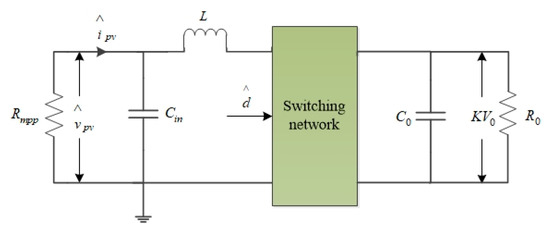
Figure 7. Small signal equivalent circuit of the boost converter.

According to Equation (26), the response of ${\stackrel{\wedge }{v}}_{pv}$ to the amplitude Δd of duty cycle disturbance $\stackrel{\wedge }{d}$ can be deduced as follows:

$${\stackrel{\wedge }{v}}_{pv}=\mu \Delta d\left[1-\frac{1}{\sqrt{1-{\xi }^2}}\exp (-\xi {\omega }_{n}T)\sin ({\omega }_{n}T\sqrt{1-{\xi }^2}+\arccos (\xi ))\right]$$

(28)

The response of $\stackrel{\wedge }{P}$ to small signal disturbance amplitude Δd can be expressed as

$$\stackrel{\wedge }{P}=-\frac{{\stackrel{\wedge }{V}}_{pv}^2}{R_{mpp}}\approx -\frac{{\mu }^2\Delta d^2}{R_{mpp}}\left\{1-\frac{1}{\sqrt{1-{\xi }^2}}\exp (-\xi {\omega }_{n}T)\sin \left[{\omega }_{n}T\sqrt{1-{\xi }^2}+\arccos (\xi )\right]\right\}$$

(29)

which is a typical second-order system. The disturbance of output power satisfies the following inequality:

$$\Delta P_0-\Delta P_{\tau }\le \stackrel{\wedge }{P}\le \Delta P_0+\Delta P_{\tau }$$

(30)

$$\Delta P_0=-\mu \Delta d^2/R_{mpp}$$

(31)

In Equation (30), ΔP_τ is the peak of the maximum overshoot of the system in the adjustment time.

According to feedback control theory, when the system has been adjusted for time T_τ, the output of the system is basically stable, and the expression of T_τ is:

$$T_{\tau }\cong -\frac{1}{\xi {\omega }_n}\ln (\tau )$$

(32)

$$\tau =\Delta P_{\tau }/\left(2\left|\Delta P_0\right|\right)$$

(33)

where τ is usually taken as a reference index for the end of the transient process. When τ < 0.03, the transient process ends. In order to prevent the MPPT algorithm from the effect caused by the inherent transient oscillation characteristics, the sampling period T_c needs to meet the following requirements:

$$T_c\ge T_{\tau }$$

(34)

It should be emphasized that Equation (34) is the constraint of the sampling period of the system output power.

According to Equations (26) and (29), the power output of the photovoltaic system is subject to an oscillation process, and the oscillation time is restricted by two factors: the inherent parameters of the system L, C_in and the resistance R_mpp corresponding to the maximum power point. In order to ensure the reliability of the MPPT algorithm and the dynamic response of the system, it is necessary to ensure that the sampling time meets Equation (34). On the basis of meeting Equation (34), the sampling period cannot be too large. The sampling time should be selected appropriately, and in this paper, it was obtained by

$$T_c\approx (2-4)T_{\tau }$$

(35)

3. Simulation Analysis

3.1. Simulation Parameters and Models

In MATLAB/Simulink, for meeting the needs of our research work in the future, two First Solar FS-4112 thin-film modules connected in series were used; their parameters are tabulated in Table 1. The simulation model of the module adopts the engineering mathematical model derived by the two-point method and its improved method. The overall system is shown in Figure 8, and the parameters are shown in Table 2.

Table 1. Thin-film module parameters.

Parameter	Value
Nominal power	112.5 W
Voltage at PMAX	68.5 V
Current at PMAX	1.64 A
Open circuit voltage	87 V
Short circuit current	1.83 A

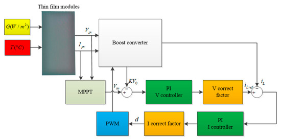
Figure 8. Schematic diagram of the system simulation.

Table 2. System parameters.

Parameter	Value
Input capacitance, Cin (μF)	600
Output capacitance, C0 (μF)	200
Inductance, L (mH)	2.4
Switching frequency, fs (kHz)	20
Output resistance, R0 (Ω)	900

3.2. Simulation Results under Fixed Irradiance

Figure 9 represents the output power of the thin-film modules under a fixed irradiance of 1000 W/m² after it turns on.

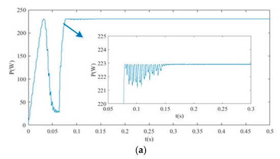
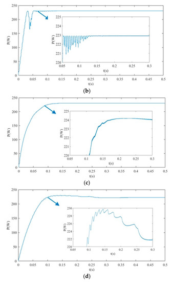
Figure 9. Comparison of four methods under a fixed irradiance: (a) perturbation-and-observation (P&O) method; (b) two-stage variable step size (2SVSS) method; (c) DCL control method; (d) the proposed approach (CCM/ discontinuous conduction mode (DCM) hybrid control method).

Figure 9a shows the results for the perturbation-and-observation (P&O) method. Because of the strict linear relationship between the output power and duty ratio of the DC-DC converter, it is difficult for the whole system to maintain a good performance in terms of the dynamic response and stability at the same time, at any step size. If the step size is too large, the tracking accuracy is reduced. If the step size is too small, it takes a long time to reach the maximum power point, especially when the light intensity changes. The time for modules to recover to the maximum power point will be very short. The vibration is also severe during the power rise. When the steady state is reached, the oscillation amplitude of the power output is larger than under the other three methods.

Figure 9b shows the results for the two-stage variable step size control strategy. Both the dynamic response and the stability at the maximum power point are obviously improved, but there is power fluctuation in the rising stage. At the same time, because the two-stage variable step control method simply uses two different steps from zero to maximum power point, it cannot meet the inherent characteristics of the system, which will lead to a large energy loss.

Figure 9c,d shows the results for the DCL control method and the proposed CCM/DCM hybrid control strategy. They adopt the same 3SVSS-MPPT algorithm but different voltage control strategies. The speed of maximum power tracking is guaranteed, because in the first stage, the voltage corresponding to the maximum power point of the module is achieved by the closed-loop control. Then a two-stage variable step-size control method is adopted near the maximum power point. When the module is working near the maximum power point, the step size of the 2nd and 3rd stage of the methods, shown in Figure 9c,d, is relatively small, the voltage at the maximum power point is stable, and the power oscillation is decreased. That is to say, the performances of these two methods are significantly improved. It should be mentioned that under fixed irradiance, the performance of the DCL control strategy is a little better than the CCM/DCM hybrid control strategy, but in other circumstances, the CCM/DCM hybrid control strategy has more advantages.

3.3. Simulation Results under Drastic Changes in Irradiance

In order to reflect the change of light intensity in the BIPV system, in Figure 10, the change of irradiance was set as follows. Within the first 0.5 s, the irradiance was 1000 W/m², and it decreased by 200 W/m² every 0.5 s until 2 s was reached. After 2 s, the irradiance increased by 200 W/m² every 0.5 s until 3.5 s.

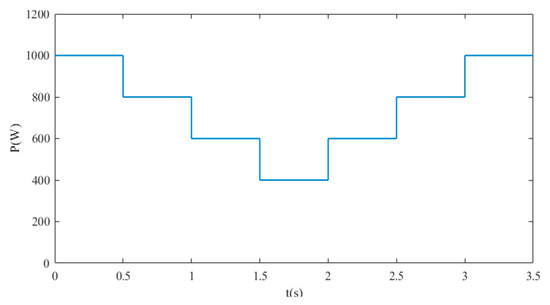
Figure 10. Simulated change of irradiance.

Figure 11 presents the simulation results of the output power of thin-film modules under the abrupt irradiance change.

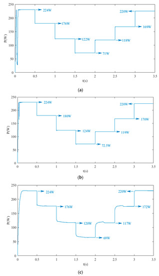
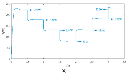
Figure 11. Comparative results of the output power of four methods under a simulated change of irradiance: (a) P&O method; (b) 2SVSS method; (c) DCL control method; (d) the proposed approach.

According to the characteristics of the module, when the irradiance changes, the current at the maximum power point of the module changes obviously, and the changing trend is almost the same as that of power, while the voltage is almost unchanged. As observed in Table 3 and Table 4, when the irradiance changed from 1000 W/m² to 400 W/m², the regulated powers by the three conventional methods were obviously lower than the theoretical value. This also means that the average powers and deviations were larger than under the CCM/DCM hybrid control strategy, especially when the irradiance was low. Compared with the three conventional methods, the most significant advantage of the CCM/DCM hybrid control strategy is high accuracy even when the irradiance is low or changes dramatically. When the irradiance changed from 400 W/m² to 1000 W/m², the CCM/DCM hybrid control strategy also had a much better performance in terms of recovering the original stable state than other methods. Among the four exhibited methods, the CCM/DCM hybrid control strategy is the only one that had good reproducibility with a deviation of no more than 1 W, as the irradiance was leaping up and down. Additionally, the CCM/DCM method delivered the most power among the four methods at a low irradiance, such as 600 and 400 W/m². This led to the highest average power being achieved by the CCM/DCM method both when the irradiance was decreasing and increasing, as exhibited in Table 3. In the whole process of irradiances change, the average power of the proposed method was the highest among the four methods. Therefore, the proposed control strategy caused less power loss than the other three methods. In another words, the control strategy proposed in this paper has a relative deviation below 2.2%, which is much lower than the other three methods, as shown in Figure 12. The relative deviation is defined as the power deviation divided by the theoretical maximum power.

Table 3. Module power (W) of various control strategies corresponding to different irradiance values.

Irradiance (W/m2)	Theoretical Maximum Power of Modules	P&O		2SVSS		DCL Control		Proposed Method
		Down	up	Down	up	Down	up	Down	up
1000	225	224	220	224	220	224	220	222	222
800	181	176	169	180	170	176	172	179	179
600	136	122	118	124	119	120	117	134	133
400	80	71	71	72.5	72.5	69	69	80	80
Average power(W)	155.5	148.25	144.5	150.13	145.38	147.5	144.5	153.75	153.5

Table 4. Deviation between the maximum power obtained by various methods and the theoretical value.

Irradiance (W/m2)	Theoretical Maximum Power of Modules	P&O		2SVSS		DCL Control		Proposed Method
		Down	up	Down	up	Down	up	Down	up
1000	225	−1	−5	−1	−5	−1	−5	−3	−3
800	181	−5	−12	−1	−11	−5	−9	−2	−2
600	136	−14	−18	−12	−17	−16	−19	−2	−3
400	80	−9	−9	−7.5	−7.5	−11	−11	0	0
Average deviation(W)	/	−7.25	−11	−5.38	−10.13	−8.13	−11	−1.8	−2

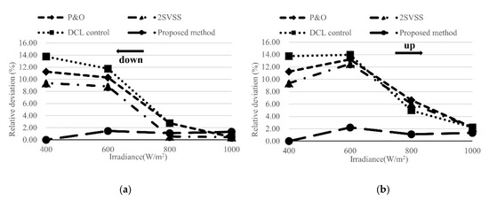
Figure 12. Comparison of the relative deviation of the four methods in the simulation: (a) the irradiance is down; (b) the irradiance is up.

Moreover, the proposed control strategy works at a higher efficiency under low irradiance, such as 400 W/m². It is the only method that could deliver the theoretical maximum power. This is particularly important for BIPVs, since the mounting angles of thin-film BIPV modules are likely perpendicular, with large deviation from the optimal elevation angle. The CCM/DCM hybrid control method could deliver more power from the thin-film modules under such conditions.

4. Experimental Validation

4.1. Description of the Experimental Setup

The overall experimental system is shown in Figure 13. In order to realize the rapid and continuous change of irradiance and maintain consistency in the simulation, a PV1000 photovoltaic simulator was utilized during debugging to substitute for the output of thin-film PV modules working under an actual light source. The parameters of the thin film in PV1000 are set the same as in Matlab. Three scenarios were simulated: working under fixed irradiance (S = 1000 W/m²), various sampling times (T_s = T_c = 100 μs, T_s = 50 μs < T_c, T_s = 200 μs), and sudden change of irradiance (the same as the condition of simulation). Other experimental parameters were the same as the simulation parameters tabulated in Table 2. The control algorithm was implemented in the TMS320F28335 control board. The data logger statement was used to obtain the experimental waveforms.

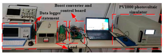
Figure 13. Experimental setup.

4.2. Experiment Results

Figure 14 shows the experimental results of the system under the fixed irradiance.

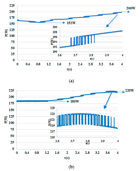
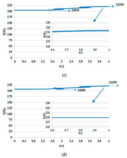
Figure 14. Comparative output power of four methods under fixed irradiance: (a) P&O method; (b) 2SVSS method; (c) DCL control; (d) the proposed approach.

When the irradiance is fixed, the experimental results confirm the simulation results and verify the advantages of the proposed CCM/DCM hybrid control strategy. As exhibited in Figure 14c,d, the rising time of the output power of the module was 3 s, which was shorter than under the other two methods, and the power oscillations within the rising time and at the maximum power point were also smaller. In terms of the P&O algorithm, the output power of the module did not reach the maximum within the test time. For the two-stage variable step method, when the modules reached the maximum power within 4 s, there were obvious oscillations and some power loss.

As shown in Figure 14c,d, the output power of the modules reached a steady state after 3 s. When the output power of the modules reaches the maximum, the oscillation state should be altered by changing the sampling period of the system, according to Equation (18). This is shown in Figure 15.

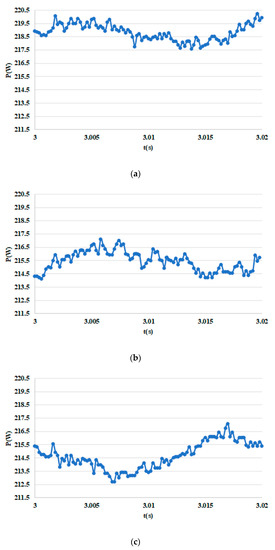
Figure 15. Test results with different sampling time T_s: (a) T_s = T_c = 100 μs meeting (18); (b) T_s = 50 μs < T_c; (c) T_s = 200 μs > T_c.

It can be seen in Figure 15 that the sampling time significantly affects the output power of the module and the stability of the MPPT algorithm. As shown Figure 15a, when the sampling period is appropriately designed, the output power of the modules is close to the theoretical value, and the oscillation near the maximum power point is about 1 W, which is relatively small. This indicates low power loss and high conversion efficiency. When the sampling time is short, there are too many transitions in the MPPT algorithm, although the oscillation of the system at the maximum power point is not more than 2 W, as shown in Figure 15b. In this case, the actual output power is slightly lower than the theoretical value, and the system efficiency is reduced. As shown in Figure 15c, if the sampling period of the system is large, the oscillation of the system at the maximum power point is nearly 3 W, and the output power is also lower than the theoretical value. The overall efficiency of the system is reduced as well.

Figure 16 shows the comparative test results for the output power of the four methods under dramatic irradiance change. These results are consistent to the simulation. When the light intensity changes dramatically, such as from 1000 W/m² to 800 W/m², only the CCM/DCM hybrid control strategy can control the output power of the modules at close to the theoretical power output value in Table 5. When the irradiance decreases dramatically in a short period of time (from 800 W/m² to 600 W/m² to 400 W/m²), it can be seen from Table 5 that the average power of the first three methods is lower than that of the proposed method. It also means that the first three control algorithms lead the output power to deviate significantly from the theoretical value, as shown in Table 6. The maximum deviation during the irradiance decreasing is 55 W. That is, their control accuracy is even worse in real applications than in the simulation, causing deterioration of the system energy efficiency. However, as shown in Figure 17, the proposed method has a relative deviation as low as 5%, which is much lower than the other three methods. What is more, the relative deviation of the CCM/DCM method remains stable between 3% and 5% for all four irradiances. When the irradiance suddenly rises again, the results are similar to those in the simulation; the proposed method has a good ability to recover the original steady state. In short, the proposed method shows a much better performance than the first three methods.

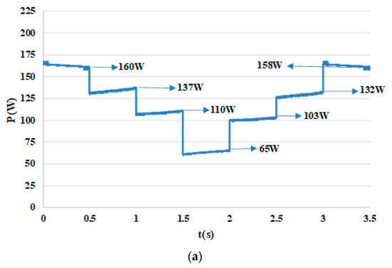
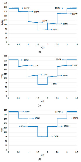
Figure 16. Output power of four methods under the dramatic irradiance change: (a) P&O method; (b) 2SVSS method; (c) DCL method; (d) the proposed method.

Table 5. Module power (W) of various control strategies corresponding to different irradiances.

Irradiance (W/m2)	Theoretical Maximum Power of Modules	P&O		2SVSS		DCL Control		Proposed Method
		Down	up	Down	up	Down	up	Down	up
1000	225	160	158	195	194	205	204	218	217
800	181	137	132	175	163	172	170	176	175
600	136	110	103	111	103	117	112	132	130
400	80	65	65	69	69	64	64	76	76
Average power (W)	155.5	118	114.5	137.5	132.25	139.5	137.5	150.5	149.5

Table 6. Deviation between the maximum power obtained by various methods and the theoretical value.

Irradiance (W/m2)	Theoretical Maximum Power of Modules	P&O		2SVSS		DCL Control		Proposed Method
		Down	up	Down	up	Down	up	Down	up
1000	225	−55	−67	−30	−31	−20	−21	−7	−8
800	181	−44	−49	−6	−18	−9	−11	−5	−6
600	136	−26	−33	−25	−33	−19	−24	−4	−6
400	80	−15	−15	−11	−11	−16	−16	−4	−4
Average deviation (W)	/	−35	−41	−18	−23.3	−16	−18	−5	−6

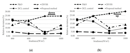
Figure 17. Comparison of the relative deviation of the four methods in this experiment: (a) the irradiance is down; (b) the irradiance is up.

Conclusively, the experimental data in Table 5 and Table 6 indicate a high tracking accuracy and energy efficiency of the CCM/DCM hybrid control strategy, compared to the other three methods. Therefore, the proposed control strategy will ensure PV system energy efficiency. Since BIPV systems operate under an irradiance lower than 1 sun and encounter in most circumstances dramatic irradiance changes, the proposed CCM/DCM hybrid control strategy is particularly suitable for BIPVs and will deliver more energy than the other three methods.

5. Conclusions

In this paper, considering the special working environment of BIPV systems and the characteristics of thin-film photovoltaic modules, a 3SVSS MPPT algorithm was proposed. This algorithm was realized by disturbing the voltage of thin-film modules. After the MPPT algorithm was introduced, a reasonable design of sampling period was introduced in this paper, so that the energy loss of the system was reduced. Lastly, a CCM/DCM hybrid control strategy based on CCM and DCM of the DC-DC converter was proposed to realize perturbing the voltage of the modules. The proposed method simplified the design of the control parameters in two modes to a certain extent and could fully guarantee the respective control performances. What is more, the proposed control strategy can be used for other DC-DC converters as well, although only the boost converter was used in this paper.

In order to reflect the advantages of the MPPT control strategy proposed in this paper, by setting a fixed light intensity in the simulation and comparing with other control algorithms (P&O, two-stage variable step size, and DCL control), the MPPT control strategy proposed in this paper demonstrated a good performance in two basic indicators of MPPT performance, namely, rapidity and stability. In order to better reflect its application advantages in BIPV systems, different irradiance conditions were considered in the simulation. The simulation results showed that the proposed algorithm has high tracking accuracy and is promising for applications in BIPVs. The experimental work further verified the proposed scheme and proved that the proposed controller is suitable for BIPV applications.

References

- Goetzler, G.; Droesch, W. Research and Development Needs for Building-Integrated Solar Technologies; EERE: Washington, DC, USA, 2014.
- Jia, T.; Dai, Y.; Wang, R. Refining energy sources in winemaking industry by using solar energy as alternatives for fossil fuels: A review and perspective. Renew. Sust. Energy. Rev. 2018, 88, 278–296. [Google Scholar] [CrossRef]
- Tian, Z.; Zhang, X.; Jin, X.; Zhou, X.; Si, B.; Shi, X. Towards adoption of building energy simulation and optimization for passive building design: A survey and a review. Energy Build. 2018, 158, 1306–1316. [Google Scholar] [CrossRef]
- Shukla, A.; Sudhakar, K.; Baredar, P. Recent advancement in BIPV product technologies: A review. Energy Build. 2017, 140, 188–195. [Google Scholar] [CrossRef]
- Femia, N.; Lisi, G.; Petrone, G.; Spagnuolo, G.; Vitelli, M. Distributed maximum power point tracking of photovoltaic arrays: Novel approach and system analysis. IEEE Trans. Ind. Electron. 2008, 55, 2610–2621. [Google Scholar] [CrossRef]
- Jayathissa, P.; Luzzatto, M.; Schmidli, J.; Hofer, J.; Nagy, Z.; Schlueter, A. Optimizing building net energy demand with dynamic BIPV shading. Appl. Energy 2017, 202, 726–735. [Google Scholar] [CrossRef]
- Cronemberger, J.; Corpas, M.; Cerón, I.; Caamaño-Martín, E.; Sánchez, S. BIPV technology application: Highlighting advances, tendencies and solutions through Solar Decathlon Europe houses. Energy Build. 2014, 83, 44–56. [Google Scholar] [CrossRef]
- Sánchez-Palencia, P.; Martín-Chivelet, N.; Chenlo, F. Modeling temperature and thermal transmittance of building integrated photovoltaic modules. Sol. Energy 2019, 184, 153–161. [Google Scholar] [CrossRef]
- Kumar, N.; Sudhakar, K.; Samykano, M. Performance evaluation of CdTe BIPV roof and façades in tropical weather conditions. Energy Sources Part A 2020, 42, 1057–1071. [Google Scholar] [CrossRef]
- Zomer, C.; Costa, M.; Nobre, A.; Rüther, R. Performance compromises of building-integrated and building-applied photovoltaics (BIPV and BAPV) in Brazilian airports. Energy Build. 2013, 66, 607–615. [Google Scholar] [CrossRef]
- Spiliotis, K.; Gonçalves, J.; Van De Sande, W. Modeling and validation of a DC/DC power converter for building energy simulations: Application to BIPV systems. Appl. Energy 2019, 240, 646–665. [Google Scholar] [CrossRef]
- Sande, W.; Daenen, M.; Spiliotis, K.; Goncalves, J.; Ravyts, S.; Saelens, D. Reliability comparison of a DC-DC converter placed in building-integrated photovoltaic module frames. In Proceedings of the 2018 7th International Conference on Renewable Energy Research and Applications (ICRERA), Paris, France, 14–17 October 2018. [Google Scholar] [CrossRef]
- Alik, R.; Jusoh, A. Modified Perturb and Observe (P&O) with checking algorithm under various solar irradiation. Sol. Energy 2017, 148, 128–139. [Google Scholar] [CrossRef]
- Bradai, R.; Boukenoui, R.; Kheldoun, A.; Salhi, H.; Ghanes, M. Experimental assessment of new fast MPPT algorithm for PV systems under nonuniform irradiance conditions. Appl. Energy 2017, 199, 416–429. [Google Scholar] [CrossRef]
- Jiang, Y.; Qahouq, J.A.A.; Haskew, T.A. Adaptive step size with adaptive-perturbation-frequency digital MPPT controller for a single-sensor photovoltaic solar system. IEEE Trans. Power Electron. 2012, 28, 3195–3205. [Google Scholar] [CrossRef]
- Dasgupta, N.; Pandey, A.; Mukerjee, A. Voltage-sensing-based photovoltaic MPPT with improved tracking and drift avoidance capabilities. Sol. Energy Mat. Sol. Cell 2008, 92, 1552–1558. [Google Scholar] [CrossRef]
- Alzate, R.; Oliveira, V.; Magossi, R. Double Loop Control Design for Boost Converters Based on Frequency Response Data. In Proceedings of the IFAC, Toulouse, France, 9–14 July 2017. [Google Scholar] [CrossRef]
- Le, H.; Orikawa, K.; Itoh, J. Circuit-parameter-independent nonlinearity compensation for boost converter operated in discontinuous current mode. IEEE Trans. Ind. Electron. 2016, 64, 1157–1166. [Google Scholar] [CrossRef]
- Forouzesh, M.; Siwakoti, Y.; Gorji, S.A.; Blaabjerg, F.; Lehman, B. Step-up DC-DC converters: A comprehensive review of voltage-boosting techniques, topologies, and applications. IEEE Trans. Power Electron. 2017, 32, 9143–9178. [Google Scholar] [CrossRef]
- Chen, Y.; Jhang, Y.; Liang, R. A fuzzy-logic based auto-scaling variable step-size MPPT method for PV systems. Sol. Energy 2016, 126, 53–63. [Google Scholar] [CrossRef]
- Liu, C.; Chen, J.; Liu, Y. An asymmetrical fuzzy-logic-control-based MPPT algorithm for photovoltaic systems. Energies 2014, 7, 2177–2193. [Google Scholar] [CrossRef]
- Yatimi, H.; Aroudam, E. Assessment and control of a photovoltaic energy storage system based on the robust sliding mode MPPT controller. Sol. Energy 2016, 139, 557–568. [Google Scholar] [CrossRef]
- Messalti, S.; Harrag, A.; Loukriz, A. A new variable step size neural networks MPPT controller: Review, simulation and hardware implementation. Renew. Sustain. Energy Rev. 2017, 68, 221–233. [Google Scholar] [CrossRef]
- Rashid, K.; Mohammadi, K.; Powell, K. Dynamic simulation and techno-economic analysis of a concentrated solar power (CSP) plant hybridized with both thermal energy storage and natural gas. J. Clean. Prod. 2020, 248. [Google Scholar] [CrossRef]
- Songwongwanich, A.; Yang, Y.; Blaabjerg, F. Delta Power Control Strategy for Multistring Grid-Connected PV Inverters. IEEE Trans. Ind. Appl. 2016. [Google Scholar] [CrossRef]
- Jain, A.; Kapoor, A. Exact analytical solutions of the parameters of real solar cells using Lambert W-function. Sol. Energy Mater. Sol. Cells 2004, 81, 269–277. [Google Scholar] [CrossRef]
© 2020 by the authors. Licensee MDPI, Basel, Switzerland. This article is an open access article distributed under the terms and conditions of the Creative Commons Attribution (CC BY) license (http://creativecommons.org/licenses/by/4.0/).