Long-Term Temperature Evaluation of a Ground-Coupled Heat Pump System Subject to Groundwater Flow


Abstract
1. Introduction
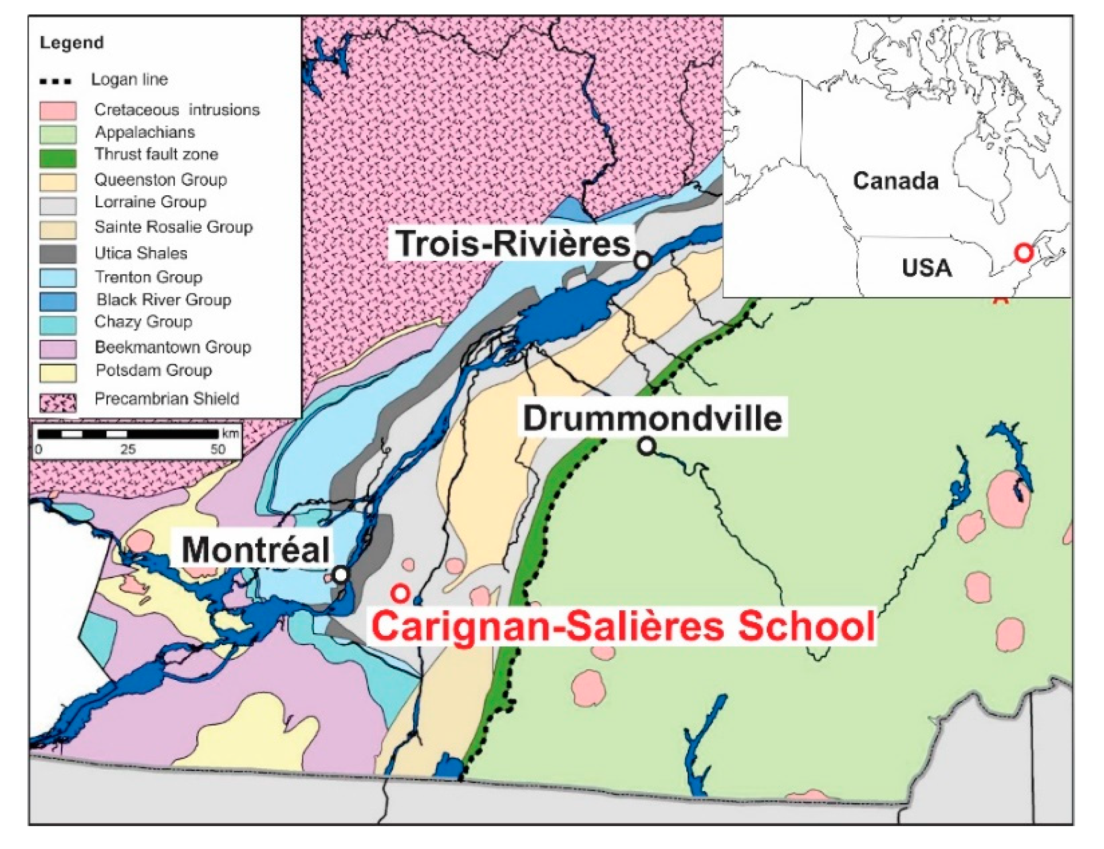
2. Site Description
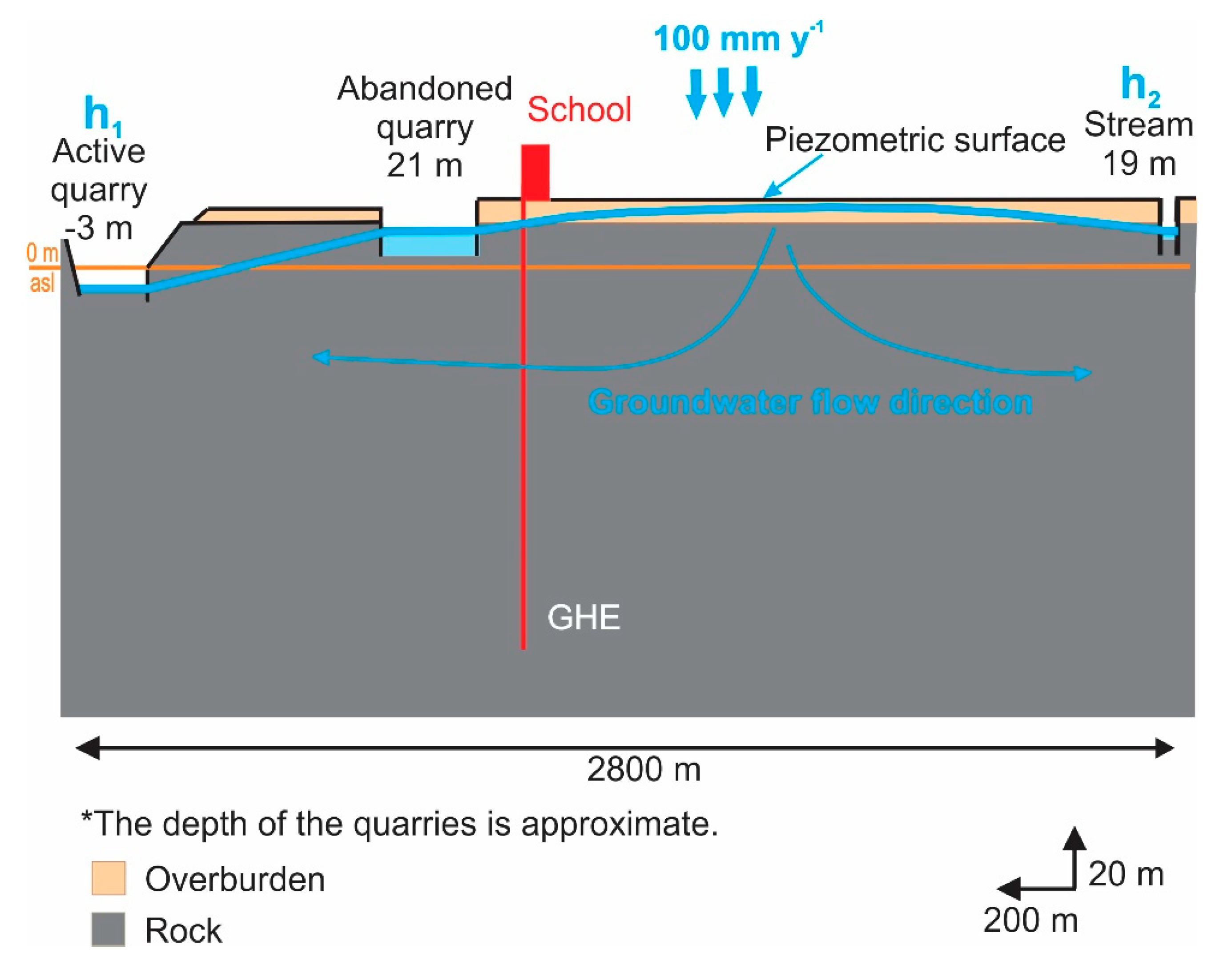
2.1. Geological and Hydrogeological Setting
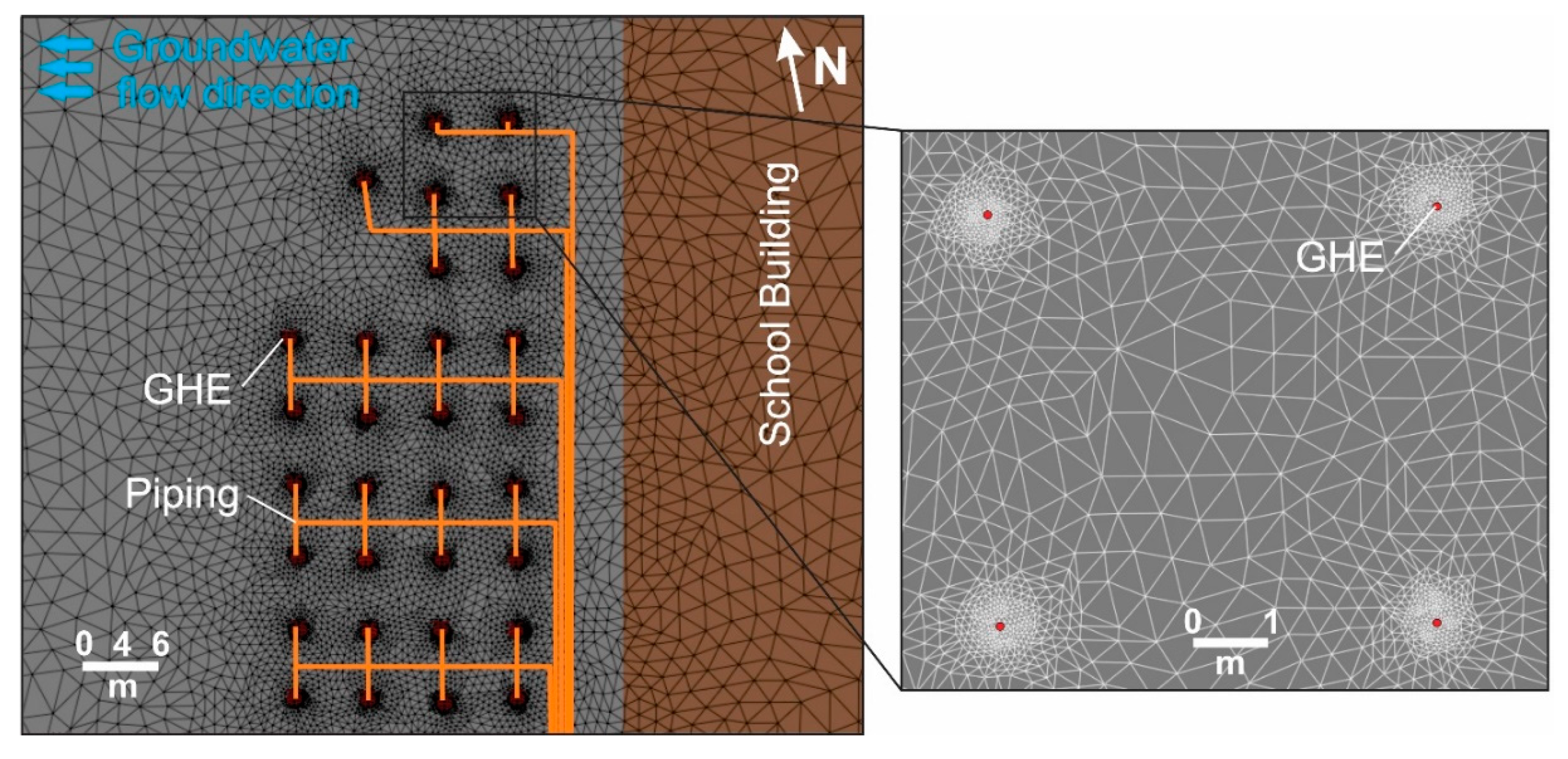
2.2. Ground Heat Exchanger Characteristics
3. Methodology
3.1. Laboratory Measurement of Thermal Conductivity
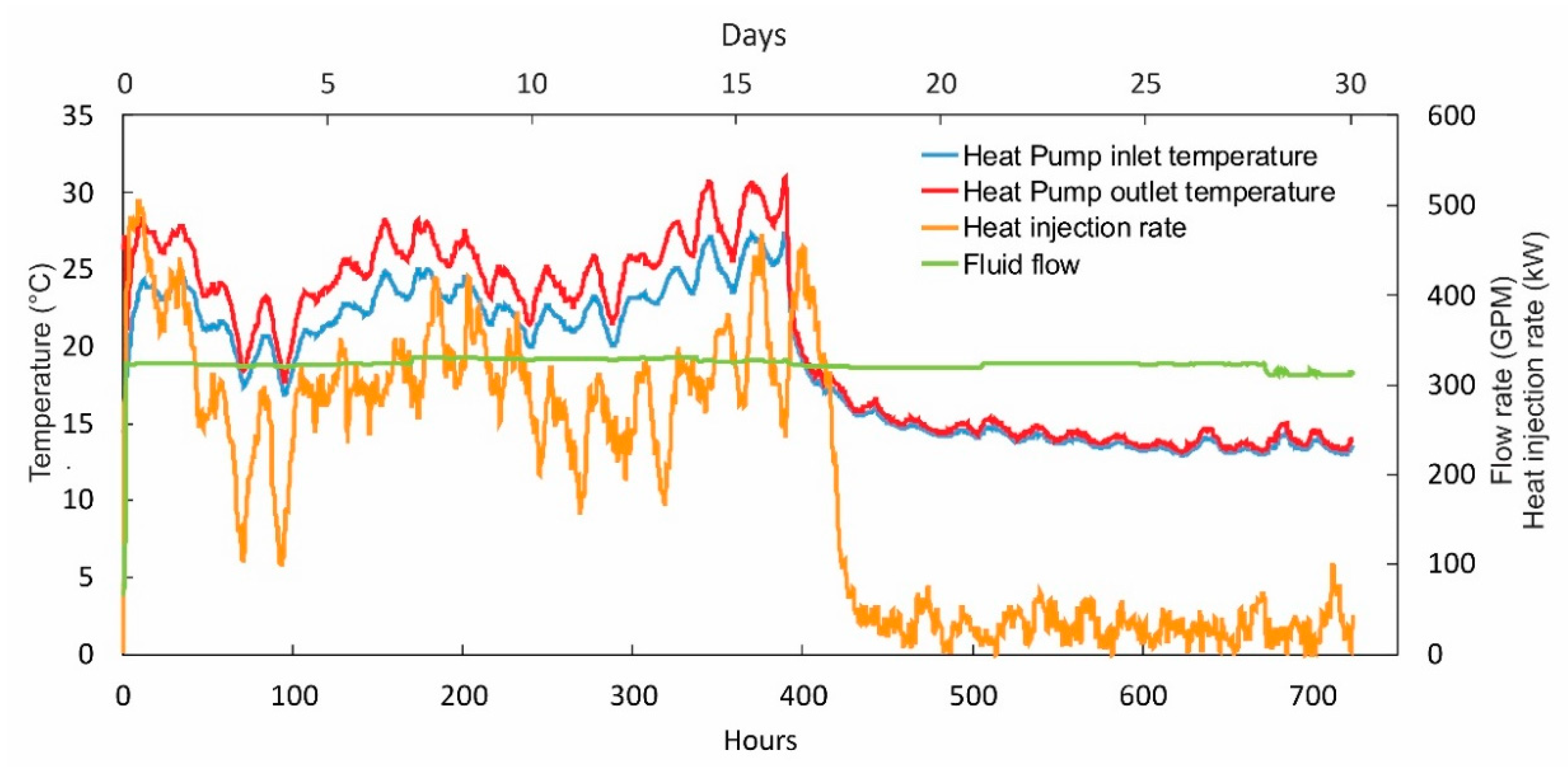
3.2. In-Situ Heat Injection Test
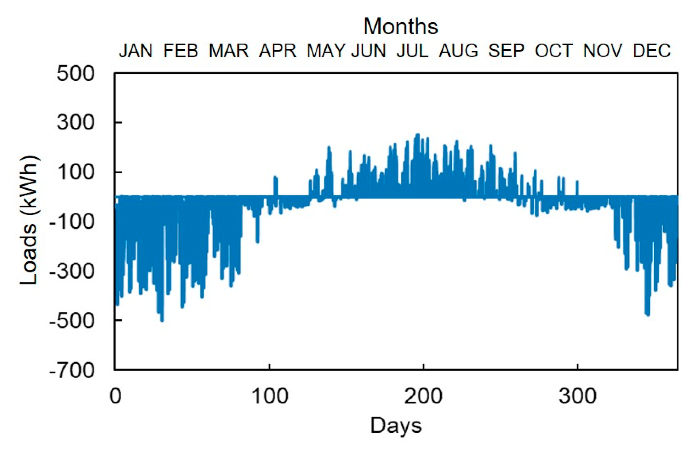
3.3. Building and Ground Load Evaluation
3.4. GCHP System Simulation
3.4.1. Governing Equations
3.4.2. Model Geometry and Properties
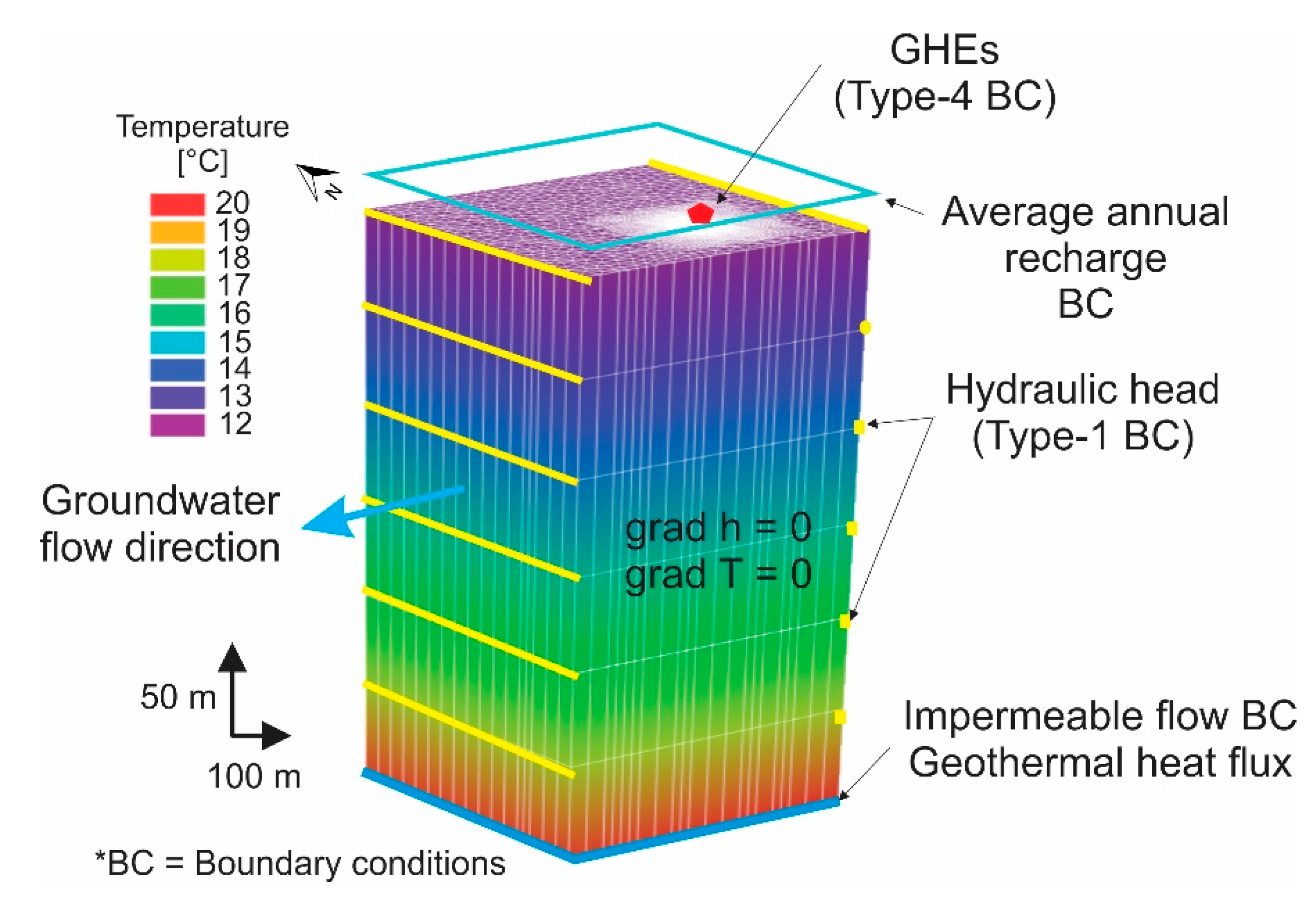
3.4.3. Initial and Boundary Conditions
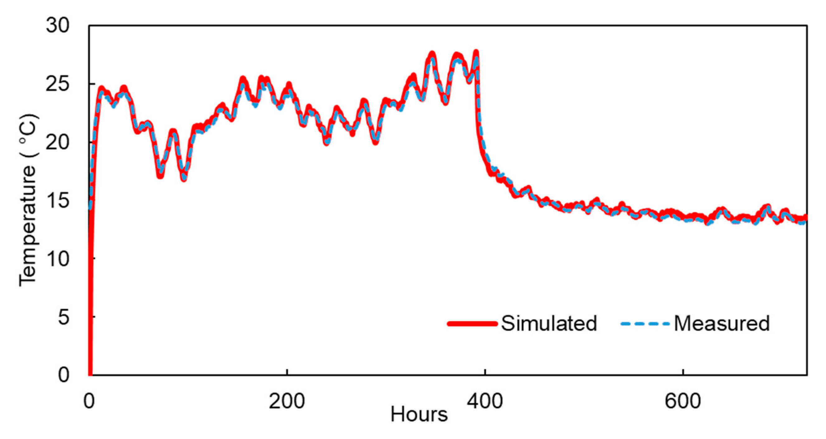
3.4.4. Model Calibration
4. Results
4.1. Groundwater Flow Conditions
4.2. Subsurface Thermal Conductivity
4.3. In-Situ Heat Injection Test
4.4. GCHP System Simulation
4.4.1. Ground Loads
4.4.2. Model Calibration
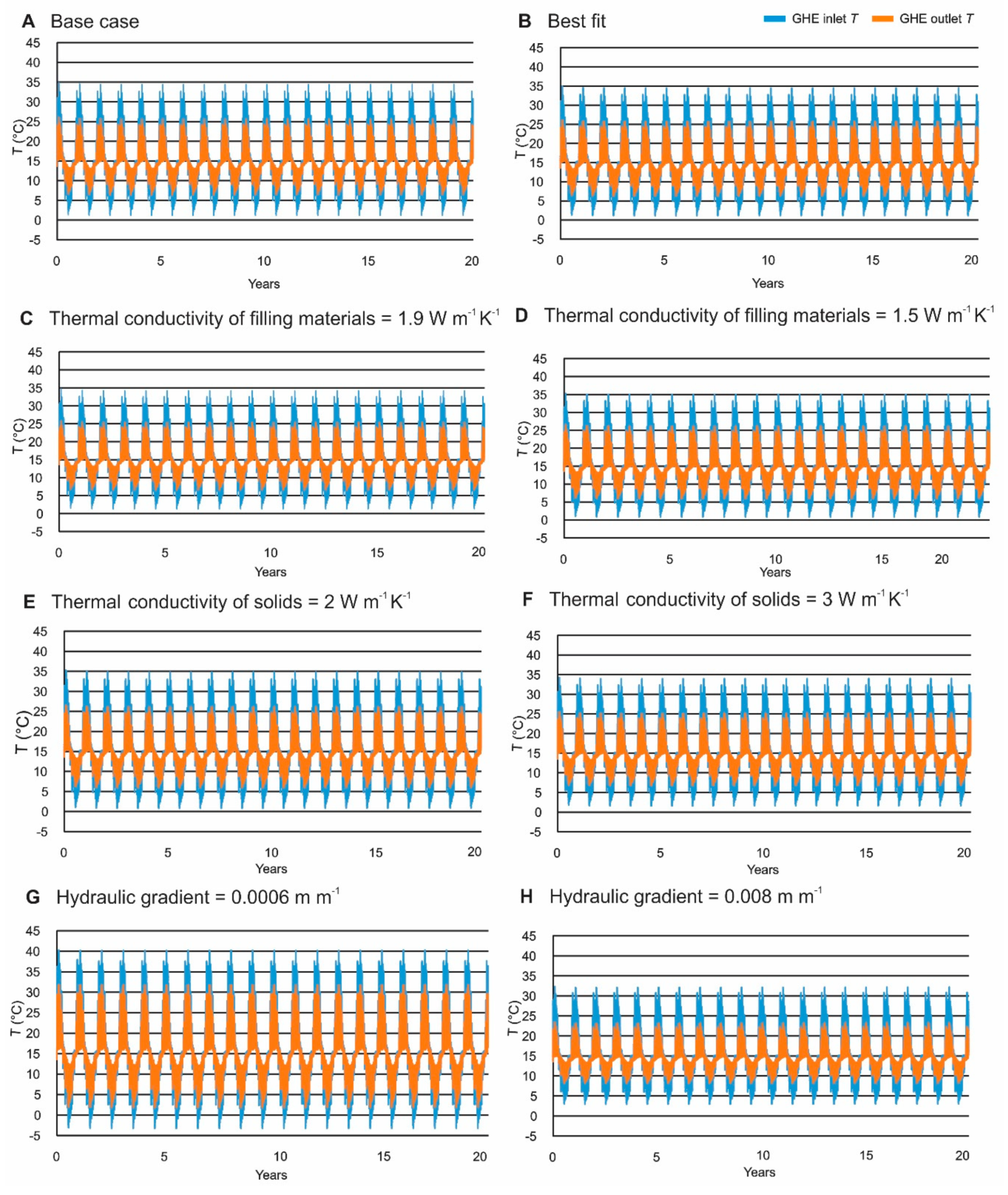
4.4.3. System Operation—Twenty-Year Simulations
5. Discussion
6. Conclusions
Author Contributions
Funding
Acknowledgments
Conflicts of Interest
Nomenclature
| c | Specific heat capacity [J kg−1 K−1] |
| COP | Coefficient of performance [−] |
| ε | Volume fraction [−] |
| H | Heat source/sink term [W m−3] |
| h | Hydraulic head [m] |
| K | Hydraulic conductivity tensor [m s−1] |
| K | Hydraulic conductivity [m s−1] |
| L | Distance [m] |
| P | Heating load [W] |
| Q | Hydraulic source/sink term [m3 s−1] |
| q | Darcy flux tensor [m s−1] |
| λ | Thermal conductivity tensor [W m−1 K−1] |
| λ | Thermal conductivity [W m−1 K−1] |
| ρ | Density [kg m−3] |
| ρc | Volumetric heat capacity [J m−3 K−1] |
| Ss | Specific storage coefficient [m−1] |
| T | Temperature [K] or [°C] |
| t | Time [s] |
| Thermal hydrodynamic dispersion tensor [W m−2 K−1] | |
| u | Heat carrier fluid velocity tensor [m s−1] |
| w | Annual recharge [m s−1] |
Subscripts
| EOB | Extended Oberbeck-Boussineq approximation |
| g | Grout |
| gw | Groundwater flow |
| il | Inlet pipe |
| ol | Outlet pipe |
| r | Heat carrier fluid |
| s | Subsurface |
Abbreviations
| asl | Above sea level |
| E | East |
| GCHP | Ground-coupled heat pump |
| GHE | Ground heat exchanger |
| MTPS | Modified transient plane source |
| TRT | Thermal response test |
| W | West |
References
- Dehkordi, S.E.; Schincariol, R.A. Effect of thermal-hydrogeological and borehole heat exchanger properties on performance and impact of vertical closed-loop geothermal heat pump systems. Hydrogeol. J. 2014, 22, 189–203. [Google Scholar] [CrossRef]
- Ferguson, G. Screening for heat transport by groundwater in closed geothermal systems. Groundwater 2015, 53, 503–506. [Google Scholar] [CrossRef] [PubMed]
- Zanchini, E.; Lazzari, S.; Priarone, A. Long-term performance of large borehole heat exchanger fields with unbalanced seasonal loads and groundwater flow. Energy 2012, 38, 66–77. [Google Scholar] [CrossRef]
- Bernier, M. Ground-coupled heat pump system simulation. ASHRAE Trans. 2001, 107, 605–616. [Google Scholar]
- Fujii, H.; Itoi, R.; Fujii, J.; Uchida, Y. Optimizing the design of large-scale ground-coupled heat pump systems using groundwater and heat transport modeling. Geothermics 2005, 34, 347–364. [Google Scholar] [CrossRef]
- Fujii, H.; Inatomi, T.; Itoi, R.; Uchida, Y. Development of suitability maps for ground-coupled heat pump systems using groundwater and heat transport models. Geothermics 2007, 36, 459–472. [Google Scholar] [CrossRef]
- Signorelli, S.; Bassetti, S.; Pahud, D.; Kohl, T. Numerical evaluation of thermal response tests. Geothermics 2007, 36, 141–166. [Google Scholar] [CrossRef]
- Bozdağ, Ş.; Turgut, B.; Paksoy, H.; Dikici, D.; Mazman, M.; Evliya, H. Ground water level influence on thermal response test in Adana, Turkey. Int. J. Energy Res. 2008, 32, 629–633. [Google Scholar] [CrossRef]
- Bauer, D.; Heidemann, W.; Müller-Steinhagen, H.; Diersch, H.J.G. Modelling and simulation of groundwater influence on borehole thermal energy stores. Effstock. In Proceedings of the 11th International Conference on Energy Storage, Stockholm, Sweden, 14–17 June 2009. [Google Scholar]
- Giordano, N.; Raymond, J. Alternative and sustainable heat production for drinking water needs in a subarctic climate (Nunavik, Canada): Borehole thermal energy storage to reduce fossil fuel dependency in off-grid communities. Appl. Energy 2019, 252, 113463. [Google Scholar] [CrossRef]
- Nguyen, A.; Pasquier, P.; Marcotte, D. Borehole thermal energy storage systems under the influence of groundwater flow and time-varying surface temperature. Geothermics 2017, 66, 110–118. [Google Scholar] [CrossRef]
- Bédard, K.; Comeau, F.-A.; Raymond, J.; Malo, M.; Nasr, M. Geothermal Characterization of the St. Lawrence Lowlands Sedimentary Basin, Québec, Canada. Nat. Resour. Res. 2017, 27, 479–502. [Google Scholar] [CrossRef]
- Raymond, J.; Sirois, C.; Nasr, M.; Malo, M. Evaluating the geothermal heat pump potential from a thermostratigraphic assessment of rock samples in the St. Lawrence Lowlands, Canada. Environ. Earth Sci. 2017, 76, 83. [Google Scholar] [CrossRef]
- Raymond, J.; BÉdard, K.; Comeau, F.-A.; Gloaguen, E.; Comeau, G.; Millet, E.; Foy, S. A workflow for bedrock thermal conductivity map to help designing geothermal heat pump systems in the St. Lawrence Lowlands, Québec, Canada. Sci. Technol. Built Environ. 2019, 25, 963–979. [Google Scholar] [CrossRef]
- Brisebois, D.; Brun, J. La Plate-Forme du Saint-Laurent et les Appalaches. Géologie du Québec; Gouvernement du Québec, Public Report MM 94 -01; Ministère des ressources naturelles: Quebec City, QC, Canada, 1994; pp. 95–120. [Google Scholar]
- Séjourné, S.; Dietrich, J.; Malo, M. Seismic characterization of the structural front of southern Quebec Appalachians. Bull. Can. Pet. Geol. 2003, 51, 29–44. [Google Scholar] [CrossRef]
- Castonguay, S.; Lavoie, D.; Dietrich, J.; Laliberté, J.-Y. Structure and petroleum plays of the St. Lawrence Platform and Appalachians in southern Quebec: Insights from interpretation of MRNQ seismic reflection data. Bull. Can. Pet. Geol. 2010, 58, 219–234. [Google Scholar] [CrossRef]
- Globensky, Y. Géologie des Basses-Terres du Saint-Laurent; Ministère de l’Énergie et des Ressources du Québec: Quebec City, QC, Canada, 1987. [Google Scholar]
- Foster, J.; Symons, D.T.A. Defining a paleomagnetic polarity pattern in the Monteregian intrusives. Can. J. Earth Sci. 1979, 16, 1716–1725. [Google Scholar] [CrossRef]
- Foland, K.A.; Gilbert, L.A.; Sebring, C.A.; Jiang-Feng, C. 40Ar/39Ar ages for plutons of the Monteregian Hills, Quebec: Evidence for a single episode of Cretaceous magmatism. GSA Bull. 1986, 97, 966–974. [Google Scholar] [CrossRef]
- Feininger, T.; Goodacre, A.K. The eight classical Monteregian hills at depth and the mechanism of their intrusion. Can. J. Earth Sci. 1995, 32, 1350–1364. [Google Scholar] [CrossRef]
- Hodgson, C.J. Monteregian Dike Rocks. Ph.D. Thesis, McGill University, Montreal, QC, Canada, 1969. [Google Scholar]
- Carrier, M.-A.; Lefebvre, R.; Rivard, C.; Parent, M.; Ballard, J.-M.; Benoit, N.; Vigneault, H.; Beaudry, C.; Malet, X.; Laurencelle, M.; et al. Portrait des Ressources en eau Souterraine en Montérégie Est, Québec, Canada; PACES Final Report R-1433; Institut national de la recherche scientifique—Centre Eau Terre Environnement: Quebec City, QC, Canada, 2013. [Google Scholar]
- Environment Canada Climate Normals 1981–2010. Available online: http://www.climat.meteo.ec.gc.ca/climate_normals/index_e.html (accessed on 20 November 2019).
- Côté, J.; Masoumifard, V.; Noreau, É. Optimizing the thermal conductivity of alternative geothermal grouts. In Proceedings of the 65th Canadian Geotechnical Conference, Winnipeg, MB, Canada, 30 September–3 October 2012. [Google Scholar]
- Leblanc, Y. Analyse d’un essai de réponse thermique—Ville de Carignan; Internal Report; Richelieu Hydrogéologie: Richelieu, QC, Canada, 2012. [Google Scholar]
- Renaud, B. Évaluation de la conductivité du sol—École Carignan-Salières; Internal Report; Géo-énergie: Boucherville, QC, Canada, 2013. [Google Scholar]
- Bristow, K.L.; White, R.D. Comparison of single and dual probes for measuring soil thermal properties with transient heating. Aust. J. Soil Res. 1994, 32, 447–464. [Google Scholar] [CrossRef]
- Barry-Macaulay, D.; Bouazza, A.; Singh, R.M.; Wang, B.; Ranjith, P.G. Thermal conductivity of soils and rocks from the Melbourne (Australia) region. Eng. Geol. 2013, 164, 131–138. [Google Scholar] [CrossRef]
- Raymond, J. Colloquium 2016: Assessment of subsurface thermal conductivity for geothermal applications. Can. Geotech. J. 2018, 55, 1209–1229. [Google Scholar] [CrossRef]
- Di Sipio, E.; Galgaro, A.; Destro, E.; Teza, G.; Chiesa, S.; Giaretta, A.; Manzella, A. Subsurface thermal conductivity assessment in Calabria (southern Italy): A regional case study. Environ. Earth Sci. 2014, 72, 1383–1401. [Google Scholar] [CrossRef]
- Harris, A.; Kazachenko, S.; Bateman, R.; Nickerson, J.; Emanuel, M. Measuring the thermal conductivity of heat transfer fluids via the modified transient plane source (MTPS). J. Therm. Anal. Calorim. 2014, 116, 1309–1314. [Google Scholar] [CrossRef]
- Decagon Services KD2 Pro thermal properties analyzer; Instruction manual, Decagon Services: Pullman, WA, USA, 2016.
- C-Therm Technologies TCi Thermal Conductivity Analyzer; Instruction Manual; C-Therm Technologies: Fredericton, NB, Canada, 2016.
- Hirsch, J.J. DOE-2.2 Building Energy Use and Cost Analysis Program. Volume 1: Basics; Lawrence Berkely National Laboratory: Berkeley, CA, USA, 2004; Available online: http://doe2.com/DOE2/index.html (accessed on 20 November 2019).
- Diersch, H.J.G.; Bauer, D.; Heidemann, W.; Schatzl, P. FEFLOW White Papers Vol. 5; DHI-WASY GmbH: Berlin, Germany, 2010. [Google Scholar]
- Diersch, H.-J.G.; Bauer, D.; Heidemann, W.; Rühaak, W.; Schätzl, P. Finite element modeling of borehole heat exchanger systems: Part 2. Numerical simulation. Comput. Geosci. 2011, 37, 1136–1147. [Google Scholar] [CrossRef]
- Eskilson, P.; Claesson, J. Simulation model for thermally interacting heat extraction boreholes. Numer. Heat Transf. 1988, 13, 149–165. [Google Scholar] [CrossRef]
- Al-Khoury, R.; Bonnier, P.G.; Brinkgreve, R.B.J. Efficient finite element formulation for geothermal heating systems. Part I: Steady state. Int. J. Numer. Methods Eng. 2005, 63, 988–1013. [Google Scholar] [CrossRef]
- Al-Khoury, R.; Bonnier, P.G. Efficient finite element formulation for geothermal heating systems. Part II: Transient. Int. J. Numer. Methods Eng. 2006, 67, 725–745. [Google Scholar] [CrossRef]
- Rühaak, W.; Renz, A.; Schätzl, P.; Diersch, H.J.G. Numerical Modelling of Geothermal Applications; World Geothermal Congress: Bali, Indonesia, 2010. [Google Scholar]
- Bauer, D.; Heidemann, W.; Müller-Steinhagen, H.; Diersch, H.-J.G. Thermal resistance and capacity models for borehole heat exchangers. Int. J. Energy Res. 2011, 35, 312–320. [Google Scholar] [CrossRef]
- Saull, V.A.; Clark, T.H.; Doig, R.P.; Butler, R.B. Terrestrial Heat Flow in the St. Lawrence Lowland of Québec. Can. Min. Metall. Bull. 1962, 65, 63–66. [Google Scholar]
- Fetter, C.W. Applied Hydrogeology, 4th ed.; Prentice Hall: Upper Saddle River, NJ, USA, 2001. [Google Scholar]
- Pasquale, V.; Verdoya, M.; Chiozzi, P. Measurements of rock thermal conductivity with a Transient Divided Bar. Geothermics 2015, 53, 183–189. [Google Scholar] [CrossRef]
- Nasr, M.; Raymond, J.; Malo, M.; Gloaguen, E. Geothermal potential of the St. Lawrence Lowlands sedimentary basin from well log analysis. Geothermics 2018, 75, 68–80. [Google Scholar] [CrossRef]
- Chiasson, A.; Rees, S.J.; Spitler, J.D. A preliminary assessment of the effects of groundwater flow on closed-loop ground-source heat pump systems. ASHRAE Trans. 2000, 106, 380–393. [Google Scholar]
- Fujimoto, M.; Fujii, H.; Nagano, K.; Hiromatsu, A. Numerical modelling of large-scale cluster of vertical ground heat exchangers. GRC Trans. 2011, 35, 1101–1105. [Google Scholar]
- Jaziri, N.; Raymond, J.; Boisclair, M. Performance evaluation of a ground coupled heat pump system with a heat injection test analysis. In Proceedings of the 69th Canadian Geotechnical Conference, Vancouver, BC, Canada, 2–5 October 2016. [Google Scholar]
- Hackel, S.; Pertzborn, A. Building on experience with hybrid ground source heat pump systems. ASHRAE Trans. 2011, 117, 271–278. [Google Scholar]
- Hellström, G. Ground Heat Storage: Thermal Analysis of Duct Storage Systems. Ph.D. Thesis, Department of mathematical physics, University of Lund, Lund, Sweden, 1991. [Google Scholar]
- Philippe, M.; Bernier, M.; Marchio, D. Sizing calculation spreadsheet–Vertical geothermal borefields. ASHRAE J. 2010, 52, 20–28. [Google Scholar]
- Morrison, A.D. GS2000tm Software. In Proceedings of the Fourth International Conference on Heat Pumps in Cold Climates, Alymer, QC, Canada, 17–18 August 2000. [Google Scholar]
- Chiasson, A.; O’Connell, A. New analytical solution for sizing vertical borehole ground heat exchangers in environments with significant groundwater flow: Parameter estimation from thermal response test data. HVAC R Res. 2011, 17, 1000–1011. [Google Scholar]
- Molina-Giraldo, N.; Blum, P.; Zhu, K.; Bayer, P.; Fang, Z. A moving finite line source model to simulate borehole heat exchangers with groundwater advection. Int. J. Therm. Sci. 2011, 50, 2506–2513. [Google Scholar] [CrossRef]


| Parameter | Value |
|---|---|
| Subsurface | |
| Specific storage | 10−4 m−1 |
| Volumetric heat capacity of water | 4.2 × 10⁶ J m−3 K−1 |
| Volumetric heat capacity of subsurface solids | 2.52 × 10⁶ J m−3 K−1 |
| Thermal conductivity of water | 0.65 W m−1 K−1 |
| GHE | |
| Pipe spacing | 0.10 m |
| Inlet and outlet pipe diameter | 0.032 m |
| Pipe thermal conductivity | 0.39 W m−1 K−1 |
| Pipe wall thickness | 0.0038 m |
| Heat carrier fluid thermal conductivity | 0.48 W m−1 K−1 |
| Heat carrier fluid density | 1033 kg m−3 |
| Rock Type | Measurement Method | Number of Samples Analyzed | Average Thermal Conductivity (W m−1 K−1) |
|---|---|---|---|
| Gabbro | Needle probe | 3 | 1.87 |
| Gabbro | MTPS | 2 | 1.82 |
| Calcarenite | MTPS | 1 | 3.58 |
| Dark shale | MTPS | 3 | 2.42 |
| Light shale | MTPS | 3 | 2.85 |
| Calibration Parameter | Possible Range | Chosen Value |
|---|---|---|
| Kx (m s−1) | 10−5–10−3 | 10−4 |
| Ky (m s−1) | 10−7–10−3 | 10−4 |
| Kz (m s−1) | 10−9–10−3 | 10−6 |
| λ borehole filling material (W m−1 K−1) | 1.5–1.9 | 1.75 |
| λ host rock solids (W m−1 K−1) | 2.1–2.4 | 2.4 |
| Porosity (%) | 3–5 | 3 |
| Scenario | Hydraulic Head at Lateral Boundaries (m) | Hydraulic Gradient (m m−1) | Thermal Conductivity of Subsurface Solids (W m−1 K−1) | Thermal Conductivity of Borehole Filling Material (W m−1 K−1) |
|---|---|---|---|---|
| A | 26–24 | 0.002 | 2.5 | 1.75 |
| B | 26–24 | 0.002 | 2.4 | 1.75 |
| C | 26–24 | 0.002 | 2.4 | 1.90 |
| D | 26–24 | 0.002 | 2.4 | 1.50 |
| E | 26–24 | 0.002 | 2.0 | 1.75 |
| F | 26–24 | 0.002 | 3.0 | 1.75 |
| G | 26–25.7 | 0.0006 | 2.4 | 1.75 |
| H | 26–22 | 0.008 | 2.4 | 1.75 |
| Scenario | Hydraulic Gradient | Thermal Conductivity of Subsurface Solids | Thermal Conductivity of Borehole Filling Material | GHE Outlet Minimum/Maximum Temperature during Year 20 | |||
|---|---|---|---|---|---|---|---|
| (%) | (%) | (%) | Heating Mode | Cooling Mode | |||
| (°C) | (%) | (°C) | (%) | ||||
| A | − | − | − | 6.4 | − | 25.6 | − |
| B | 0 | −4 | 0 | 6.4 | 0 | 25.6 | 0 |
| C | 0 | −4 | 9 | 6.5 | 2 | 25.4 | −1 |
| D | 0 | −4 | −14 | 6.1 | −5 | 26.1 | 2 |
| E | 0 | −20 | 0 | 6.1 | −5 | 26.0 | 2 |
| F | 0 | 20 | 0 | 6.9 | 8 | 25.1 | −2 |
| G | −70 | −4 | 0 | 2.0 | −69 | 31.7 | 24 |
| H | 300 | −4 | 0 | 8.3 | 30 | 23.1 | −10 |
© 2019 by the authors. Licensee MDPI, Basel, Switzerland. This article is an open access article distributed under the terms and conditions of the Creative Commons Attribution (CC BY) license (http://creativecommons.org/licenses/by/4.0/).
Share and Cite
Jaziri, N.; Raymond, J.; Giordano, N.; Molson, J. Long-Term Temperature Evaluation of a Ground-Coupled Heat Pump System Subject to Groundwater Flow. Energies 2020, 13, 96. https://doi.org/10.3390/en13010096
Jaziri N, Raymond J, Giordano N, Molson J. Long-Term Temperature Evaluation of a Ground-Coupled Heat Pump System Subject to Groundwater Flow. Energies. 2020; 13(1):96. https://doi.org/10.3390/en13010096
Chicago/Turabian StyleJaziri, Nehed, Jasmin Raymond, Nicoló Giordano, and John Molson. 2020. "Long-Term Temperature Evaluation of a Ground-Coupled Heat Pump System Subject to Groundwater Flow" Energies 13, no. 1: 96. https://doi.org/10.3390/en13010096
APA StyleJaziri, N., Raymond, J., Giordano, N., & Molson, J. (2020). Long-Term Temperature Evaluation of a Ground-Coupled Heat Pump System Subject to Groundwater Flow. Energies, 13(1), 96. https://doi.org/10.3390/en13010096