Full Coverage of Optimal Phasor Measurement Unit Placement Solutions in Distribution Systems Using Integer Linear Programming

Abstract

Integer linear programming (ILP) has been widely applied to solve the optimal phasor measurement unit (PMU) placement (OPP) problem for its computational efficiency. Using ILP, a placement with minimum number of Phasor Measurement Units (PMUs) and maximum measurement redundancy can be obtained while ensuring system observability. Author response: please delete this above sentence. However, the existing ILP-based OPP methods does not guarantee full coverage of solutions to the optimization problem, which may sequentially results in suboptimal supervision of the system. In this paper, a hybrid ILP-based method is proposed to cover all solutions to the OPP problem without any omission. Comparing with the existing exhaustive searching methods, the proposed method is more computationally efficient, which makes finding all solutions in a large system a more feasible problem.

1. Introduction

A phasor measurement unit (PMU) is able to provide voltage and current phasor measurements, which are linear in the system states (Bus voltage phasor) [1]. Therefore, the use of PMUs at each bus will lead to simplified linear state estimation [2]. Since a PMU is able to measure the voltage phasor at the installed bus as well as current flow along lines incident to the installed bus, it is possible to observe the entire system by instrumenting a subset of system buses with PMUs [3]. This requires strategic placement of PMUs among the system buses. Optimal placement of PMU (OPP) aims at finding a minimum number and the optimal locations of PMUs to make the system topologically observables [1]. The main objective of placement algorithms is to guarantee full system observability with a minimum number of measurements in order to minimize the total installation cost [2].

Many OPP algorithms have been well documented since the pioneer work of Baldwin in 1993 [1,4,5,6,7,8,9]. Integer linear programming (ILP) is a fast and easy-to-implement algorithm which has long been used to solve the OPP problem. In [3], the authors used a numerical implementation of ILP for the network analysis, and for the cost of PMU installation with mixed measurement sets which included conventional power flow and the injection measurements is reported. It dealt with zero injection through an approximation way. The description of a simple modified ILP-based optimal placement method, ensuring complete topological observability of the system under intact and critical contingency cases, is presented in [10]. Gou used an integer programming technique accounting for power networks with and without conventional power flow and injection measurements [11]. This concept was extended in [12] to consider zero-injection buses, incomplete observability and measurement redundancy. The aforementioned literatures have not considered the multiple solutions to the OPP problem. In [13], a procedure for multistage PMU placement in a given time horizon using an ILP framework is presented. Two indices are proposed to further rank these multiple solutions, i.e., the bus observability index (BOI) and the system observability redundancy index (SORI). However, it is possible that multiple solutions exist even after ranking using SORI, which have not been considered in [13].

In practice, it is possible that multiple solutions, while equally optimal in terms of PMU number and SORI, can be further distinguished by other criteria that cannot be integrated in the ILP optimization problem. In the field of OPP, it is likely that two placement strategies having the same number of PMUs and SORI have different performance in other aspects such as robustness or state estimation (SE) variance that cannot be easily implemented in the objective function [14]. For example, the state estimation variance cannot be expressed directly by the locations of PMUs. Moreover, it is possible that some specific buses have higher priority to be installed with a PMU such as critical buses, generator buses and tie-line buses, but the priority is not easy to be quantified and integrated into the objective function. Hence, obtaining all the solution efficiently will allow the decision maker to examine and select the overall best solution, taking into consideration the factors that are mathematically difficult to express, without suffering any deterioration in the objective function.

The multiple solutions issue has been mentioned in [15,16], but full coverage of optimal solutions is not considered. Hitherto, there has not been a method that identifies all alternative optimal solutions to the OPP problem besides the exhaustive search method, which is extremely time consuming and not practical for large scale systems. In this paper a hybrid method is proposed to address the multiple solutions to the OPP problem. The most important contribution of the proposed hybrid method lies in its ability to locate all the optimal solutions without resorting to exhaustive search. It is able to identify all the solutions that achieve maximum SORI with minimum number of PMUs efficiently. A novel method is proposed to catagorize the network buses into three categories, and one of these categories is further analyzed to find the missing optimal solutions. Results show that the proposed method does not overlook solutions that satisfy the given critera. The proposed method has been tested on the IEEE 33, IEEE 34 and IEEE 123 bus systems, and the results show that the proposed method is able to give all the optimal solutions efficiently, even for large scale systems.

The rest of this paper is organized as follows: Section 2 introduces the formulation of the OPP, as well as how ILP is used to solve the OPP in the literatures. The proposed method is presented in detail in Section 3. It is tested on several standard systems and the results are discussed in Section 4. Concluding remarks are drawn in Section 5.

2. Optimal PMU Placement

This section introduces the preliminary knowledge of OPP including the indices to evaluate the placement and the generic expression of OPP problem. ILP is introduced and a tutorial example is given to show the application of ILP in OPP. Author response: please delete the above sentence.

2.1. Formulation of the OPP Problem

A PMU can measure not only the voltage phasor at the installed bus but also all incident currents. With network topology information, the adjacent buse’s voltage can be calculated. OPP allows a minimum number of PMUs to be used to observe a bus network in its entirety. The input of the OPP is the topology of a network and the output is a subset of the network buses. In OPP, it is possible that multiple solutions having the same number of PMUs exist. In this case, two indices are proposed to evaluate the quality of these solutions, the bus observability index (BOI) and the SORI [17].

In BOI, ${\beta }_i$ is defined as the times that bus i is observed, and equals to the number of PMUs observing bus i. Note that the maximum bus observability index is limited to maximum connectivity ${\eta }_i$ of a bus plus one, which happens only when all adjacent buses and the bus itself is equipped with PMUs.

$${\beta }_i\le {\eta }_i+1$$

(1)

SORI can be obtained by simply adding up BOI at all buses in the system. Higher SORI value indicates that the PMU-based monitoring system is more reliable. The SORI can be calculated by the following equation:

$$\gamma ={\displaystyle \sum _{i=1}^n}{\beta }_i.$$

(2)

Therefore, the OPP problem can be formulated as:

$$\begin{array}{c}\underset{N_P}{min}\left\{max\gamma (N_P,S\left(N_P\right))\right\}\hfill \\ \mathrm{s}.\mathrm{t}.O_{bs}(N_P,S\left(N_P\right))=1,\hfill \end{array}$$

(3)

where $N_P$ is the minimum number of PMUs, $S\left(N_P\right)$ is a set of bus indices where the $N_P$ PMUs are installed, $\gamma (N_P,S\left(N_P\right))$ is the redundancy measurement index and $O_{bs}$ is the observability evaluation logical function [9].

2.2. Integer Linear Programming

Integer programming is a mathematical programming method of solving an optimization problem in which some or all of the variables are restricted to integers. A linear objective function and constraints lead to ILP. When applied to solve the OPP problem, ILP is efficient in minimizing the number of PMUs while ensuring system observability. Besides, it is efficient in maximizing SORI given a specific number of PMUs. While guaranteeing observability of the system, the two objectives of the optimization problem, i.e., minimizing the PMU number and maximizing SORI, are in conflict and cannot be included in a single cost function. The minimization of the PMU number is an objective with higher priority, thus is solved in the first step and used as a constraint in the second step of the optimization problem.

The minimization of PMU number is the essential objective and an additional constraint for maximization of SORI. Therefore, the original optimization problem is divided into two optimization problems that are solved sequentially. There are two steps involved when ILP is applied to solve the OPP problem formulated in Equation (3):

• Minimizing the number of PMU while ensuring system observability.
• Maximizing the SORI using limited number of PMUs.

Step (i) can be summarized in the following equation.

$$\begin{array}{c}\underset{\mathbf{x}}{min}{\mathit{f}}^{\mathit{T}}\mathit{x}\hfill \\ \mathrm{s}.\mathrm{t}.\mathit{Ax}\ge \mathit{b},\hfill \end{array}$$

(4)

where $\mathit{f}={[1,1,\dots ,1]}^T$, f is set as a unit vector such that the objective function $f^{T}x$ indicates the number of PMU allocated, $\mathit{x}$ is a binary decision variable vector indicating whether a PMU is placed at a bus; $\mathit{A}$ is the system connectivity matrix, so $\mathit{Ax}$ indicates how many PMUs are observing a bus; $\mathit{b}$ is a all ‘1’ vector; $\mathit{Ax}\ge$ is the system observability constraint.

Step (i) above will lead to a solution $\mathit{x}$. The number of ‘1’s in the solution is the minimum number of PMUs ensuring the system observability. This result will be included in Step (ii) as an additional constraint. Step (ii) is summarized in the following equation. This step aims at maximizing the system observability redundancy index.

$$\begin{array}{c}\underset{\mathit{x}}{max}{\mathit{g}}^{\mathit{T}}\mathit{x}\hfill \\ \mathrm{s}.\mathrm{t}.\left\{\begin{array}{c}\mathit{Ax}\ge \mathit{b}\hfill \\ {\mathit{A}}_{\mathit{eq}}\mathit{x}={\mathit{b}}_{\mathit{eq}}\hfill \end{array}\right.,\hfill \end{array}$$

(5)

where ${\mathit{A}}_{\mathit{eq}}=[1,1,\dots ,1]$ and $\mathit{g}={[g_1,g_2,\dots ,g_n]}^T$ is the coefficient vector to maximize SORI, $g_i$ is equal to the number of incident lines of bus i plus 1, which is the BOI of each bus ${\beta }_i$. Hence the objective function ${\mathit{g}}^{\mathit{T}}\mathit{x}$ indicates the SORI. The objective function ${\mathit{g}}^{\mathit{T}}\mathit{x}$ indicates the SORI, while $b_{eq}$ is the number of PMU as determined in step (i). After these two steps, an optimal placement strategy can be deduced.

3. Proposed Method to Identify All the Optimal Solutions

We propose in this work a hybrid method that is based on the ILP algorithm and exhaustive search to identify all optimal solutions that provide full observability of a system with minimum number of PMUs and maximum SORI. The proposed method incorporates several steps after two steps are applied to minimize the number of PMU and maximize SORI successively. The complete process is summarized as follows:

(1)

Minimization of number of PMU using ILP. This step has been explained in detail in Section 2.2. The minimum number of PMU obtained in this step is denoted as N and included in following step as the second constraint as shown in Equation (5).

(2)

Generating multiple solutions that maximize the SORI. These multiple solutions may not cover all the optimal solutions that maximizes the SORI, so the next few steps are designed to locate all the optimal solutions.

(3)

Classification of network buses according to multiple solutions is obtained in Step (2).

(4)

Grouping of uncertain buses and forming subnetworks.

(5)

Optimization of each subnetwork in an exhaustive manner.

(6)

Summarize the placement strategy and list all the optimal solutions.

Step (1) has been explained in detail in Section 2.2. Denote the minimum number of PMU with N and an additional constraint is included in Step (2).

3.1. Generating Multiple Solutions

Step (2) in the proposed method that serves to generate multiple solutions that maximize the SORI. In this step, a small disturbance $\Delta$ is added to each entry of the coefficient $\mathit{g}$. The original $\mathit{g}$ equals the BOI of bus i${\beta }_i$ and is given by $\mathit{g}={[g_1,g_2,\dots ,g_n]}^T$.

With $0<\Delta <1$, these multiple solutions obtained will lead to the same optimal objective value when $\Delta$ is removed, which means that these different solutions are alternative optimal solutions for the original problem. The detailed proof is given in Appendix A.1.

Equation (6) lists a series of modified coefficient $\mathit{g}$ and how they are constructed. The overline above the symbol $\mathit{g}$ indicates that it is a modified coefficient, and the superscript indicates which entry of $\mathit{g}$ is modified.

$$\begin{array}{cc}\hfill {\overline{\mathbf{g}}}^1=& {[g_1+\Delta ,g_2,\dots ,g_n]}^T\hfill \\ \hfill {\overline{\mathbf{g}}}^2=& {[g_1,g_2+\Delta ,\dots ,g_n]}^T\hfill \\ \hfill \hspace{1em}& ⋮\hfill \\ \hfill {\overline{\mathbf{g}}}^n=& {[g_1,g_2,\dots ,g_n+\Delta ]}^T.\hfill \end{array}$$

(6)

In order to avoid missing any solutions, an opposite sign disturbance is also added to the coefficient as follows.

$$\begin{array}{cc}\hfill {\overline{\mathbf{g}}}^{n+1}=& {[g_1-\Delta ,g_2,\dots ,g_n]}^T\hfill \\ \hfill {\overline{\mathbf{g}}}^{n+2}=& {[g_1,g_2-\Delta ,\dots ,g_n]}^T\hfill \\ \hfill \hspace{1em}& ⋮\hfill \\ \hfill {\overline{\mathbf{g}}}^{2n}=& {[g_1,g_2,\dots ,g_n-\Delta ]}^T.\hfill \end{array}$$

(7)

These modified coefficients are used to maximize the SORI as shown in Equation (5), where the two constraints stand for system observability and the number of PMU as determined in step (1). We then obtained $2n$ solutions corresponding to the $2n$ different coefficients $\overline{\mathit{g}}\mathit{x}$. Note that boldface letter with a superscript indicates a solution which is generated by adding a small disturbance to the corresponding entry of $\mathit{g}$, while the subscript denotes an entry in the solution:

$${\mathit{x}}^{\mathbf{1}},{\mathit{x}}^{\mathbf{2}},\dots ,{\mathit{x}}^{\mathit{n}},{\mathit{x}}^{\mathit{n}+\mathbf{1}},{\mathit{x}}^{\mathit{n}+\mathbf{2}},\dots ,{\mathit{x}}^{\mathbf{2}\mathit{n}},$$

(8)

and these $2n$ solutions have the following features:

• It is possible that some solutions are identical with some other, which means that the number of actual solutions could be less than $2n$.
• If multiple solutions exist for the original problem, ${\mathit{x}}^{\mathbf{1}}$ to ${\mathit{x}}^{\mathbf{2}\mathit{n}}$ would NOT be identical. In other words, more than one distinct solution will be obtained by step (2) as long as multiple solutions exist for this problem.
• Solutions ${\mathit{x}}^{\mathbf{1}}$ to ${\mathit{x}}^{\mathbf{2}\mathit{n}}$, irrespective of whether they are identical, are solutions to the original optimization problem which has the original coefficient $\mathit{g}$, and that they share the same maximized value of SORI. The proof is given in Appendix A.1.
• Finally, ${\mathit{x}}^{\mathbf{1}}$ to ${\mathit{x}}^{\mathbf{2}\mathit{n}}$ may not cover all the multiple solutions to the original problem. In other words, some alternative optimal solutions could be missing from the collection of ${\mathit{x}}^{\mathbf{1}}$ to ${\mathit{x}}^{\mathbf{2}\mathit{n}}$.

So far, some optimal solutions have been identified. However, the aim of this work is to find all the optimal solutions. These multiple solutions obtained can provide an indication on how the other missing optimal solutions can be located. Additional steps are proposed, as outlined in the next section, to help identify all other missing optimal solutions.

3.2. Classification of Network Buses

From the obtained multiple solutions, some patterns can be identified. For example, some locations are never assigned with a PMU no matter how the coefficient $\mathit{g}$ changes, while some locations that are always assigned with a PMU irrespective of the coefficient $\mathit{g}$. On the other hand, there are some locations that are assigned with a PMU in some solutions but not in other solutions. The buses in the network are classified into three categories based on the above observations:

• The first category includes those buses that are allocated with PMUs in each of these multiple solutions. These buses are called primary buses and they form the set $\gamma$.
• The second category includes those buses that are not allocated with PMUs in each of these multiple solutions. These buses are called trivial buses and they form the set $\xi$.
• The rest of the system buses are classified into the third category. These buses are allocated PMUs in some of these multiple solutions, but are not allocated PMUs in the other multiple solutions. These buses are called uncertain buses and they form the set $\lambda$.

The reason to make such a classification is that the missing optimal solutions can be located by further analyzing the uncertain buses group. It will be proven that the missing alternative optimal solutions also obey the classification in Appendix A.2. Sets $\gamma$, $\xi$ and $\lambda$ are defined based on the multiple solutions obtained in the previous steps. Next, another three sets $\Gamma$, $\Xi$ and $\Lambda$ are defined as follows: If a bus is assigned with a PMU in all the optimal solutions, not limited to the optimal solutions found in step (2) and including potential missing optimal solutions, it is an element of the set $\Gamma$; if a bus is not assigned with a PMU in any of all the optimal solutions, it is an element of the set Ξ; if a bus is assigned with a PMU in some, but not all of the optimal solutions, it is an element of the set $\Lambda$. It can be proven that the sets $\gamma ,\xi$ and $\lambda$ are identical to the sets $\Gamma ,\Xi$ and $\Lambda$ respectively as will be shown in the Appendix A.2.

Therefore, the sets $\Gamma ,\Xi$ and $\Lambda$ can be identified using step (3). The information about the category of buses is then used to further find the solutions exhaustively. After analyzing these uncertain buses, it is found that these buses are usually distributed as cluster(s). Next, step (4) is executed to group the uncertain buses.

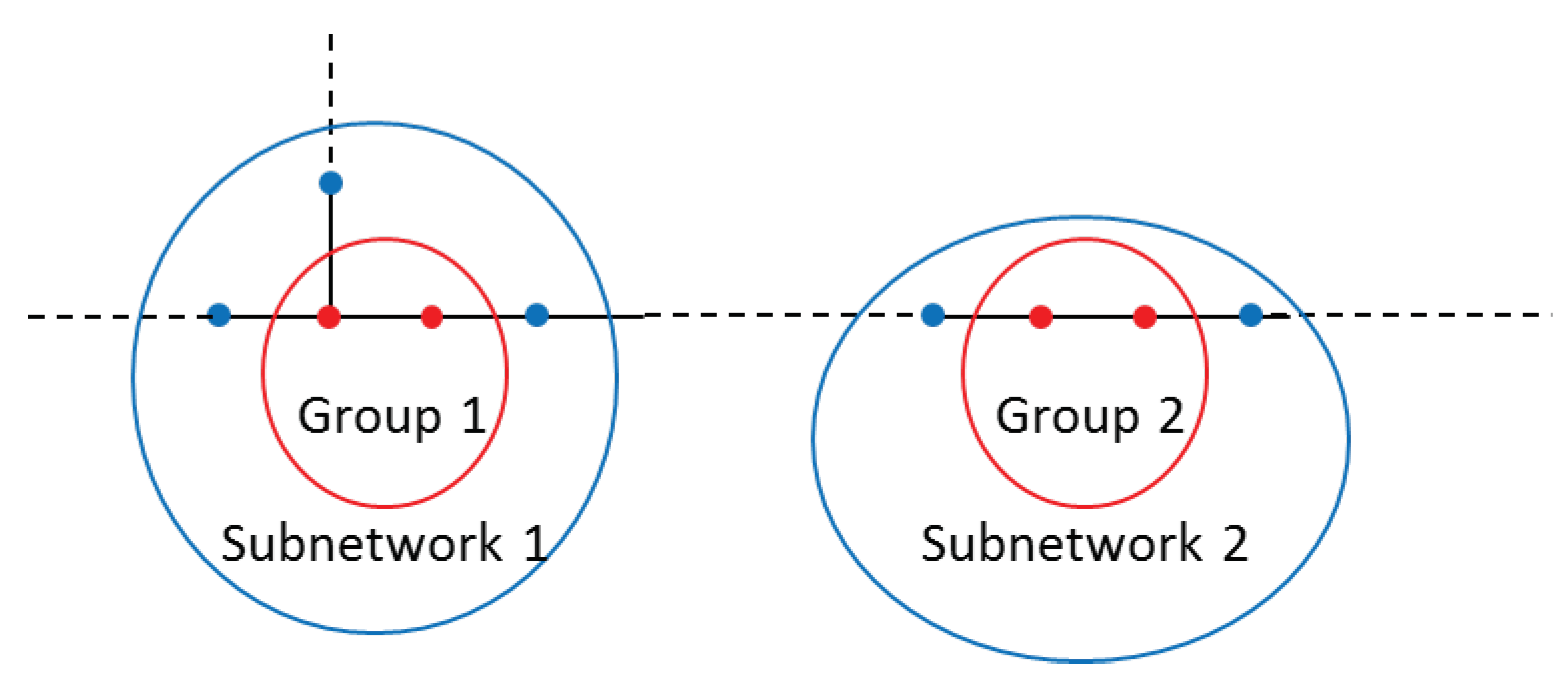
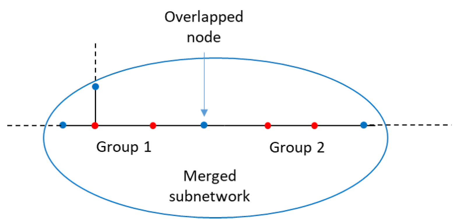
3.3. Group of Uncertain Buses

Uncertain buses are divided into independent groups that are isolated geographically. In the set $\Lambda$, it is very likely that one bus is adjacent to another and these adjacent buses are grouped together. Grouping is accomplished using the system connectivity matrix. Next is to determine the placement of PMUs among those uncertain buses. However, those buses connected to the uncertain buses will also be affected in terms of observability and measurement redundancy. Therefore, a subnetwork is formed for each group, which is made up of the uncertain nodes in the group, as well as the connected nodes. Due to the geographically isolation of each group, no matter how the PMUs are allocated in a group, only the subnetwork will be affected. The remaining part of network will not be affected, in terms of both observability and SORI. If two subnetworks are overlapped, then they are joined together to form a larger subnetwork.

The grouping of uncertain buses and subnetwork is illustrated in Figure 1. The red dots represent the uncertain buses, and the blue dots do not belong to $\Lambda$, but are connected to the uncertain buses. The red and blue dots together form a subnetwork. When conducting the optimization of each subnetwork, while the candidate locations are the uncertain buses, but the observability of the whole subnetwork should be considered. Taking the subnetwork 1 shown in Figure 1 as an example, although only two red dots are the candidate locations of the PMUs, however, the observability of the five dots (two red and three blue) need to be considered when searching for optimal placement.

Figure 1. Groups and subnetworks.

It is possible that two subnetworks have an overlap. In this case, the overlapped subnetworks are merged together to form a larger subnetwork. The merging does not affect the candidate locations. Figure 2 illustrates the merging process of two subnetworks which have a common node. This merged subnetwork consists of eight buses among which there are four candidate buses.

Figure 2. Merging overlapped subnetworks.

3.4. Subnetwork Optimization

After subnetworks are formed, optimization is carried out for each subnetworks. The optimization process for each subnetwork consists of two steps: minimization of PMU number with the observability constraint and maximization of SORI with the minimum number fixed. The minimum number of PMUs required for each subnetwork can be easily determined using the ILP algorithm:

$$\begin{array}{c}\underset{{\mathit{x}}_{sub}}{min}{\mathit{f}}_{sub}^T{\mathit{x}}_{sub}\hfill \\ \mathrm{s}.\mathrm{t}.{\mathit{A}}_{sub}{\mathit{x}}_{sub}\ge {\mathit{b}}_{sub},\hfill \end{array}$$

(9)

where ${\mathit{f}}_{\mathit{sub}}={[1,1,\dots ,1]}^T$ is a set such that the objective function ${\mathit{f}}_{\mathit{sub}}^{\mathit{T}}{\mathit{x}}_{\mathit{sub}}$ is the number of PMUs allocated, ${\mathit{x}}_{sub}$ is a binary decision variable vector indicating whether a PMU is placed at a bus and ${\mathit{A}}_{sub}$ is the corresponding matrix that indicates the connection of candidate locations and all nodes in a subnetwork. Since a subnetwork consists of a group of uncertain buses and buses connected to uncertain buses, a subnetwork has more nodes than the number of candidate locations. Therefore, the matrix ${\mathit{A}}_{sub}$ usually is not a square matrix.

Note that formulation of ${\mathit{b}}_{\mathit{sub}}$ is not the same as the formulation of $\mathit{b}$ in Equation (4), where $\mathit{b}$ is a unit vector (all ‘1’ vector) to ensure that every node in a network is observable. As a subnetwork is not a standalone network, it is a part of the whole network and has connection with other part of the network, it is possible that some of the buses in a subnetwork are already observed by a PMU outside this subnetwork. Nonetheless, those buses are still included in the subnetwork because they have impact on the SORI.

After applying all these steps, all the alternative optimal placement of the network can be obtained. The minimum number of PMU required to make the system observable is determined as N, and their placements should follow the steps below to achieve maximum SORI:

• All the primary buses are assigned PMUs. Since the number of primary buses is less than the minimum number of PMU, there will be some PMUs remain unassigned.
• The remaining PMUs are allocated to each subnetwork. Based on the optimization results for individual subnetwork, it is known how many PMUs should be assigned to each subnetwork and how they should be placed to render the subnetwork observable and achieve the maximum SORI.

One can list all the placement strategies that ensures the minimum number of PMU and maximum SORI following the above steps. Since all the subnetworks are geographically isolated, the placement in each subnetwork does not affect the other subnetwork.

3.5. OPP Considering PMU Loss

The solutions generated by previous steps guarantee the system observability under normal operating condition. However, in case of branch outage or PMU loss, the system observability is not guaranteed. Although PMU are highly reliable, they are prone to failure. In order to account for PMU loss, the system observability constraints in Equations (4) and (5) need to be modified.

In Equations (4) and (5), vector $\mathit{b}$ is set to 1, which practically means that each bus is observed by at least one PMU. If it is expected that the system remains fully observable in presence of single PMU loss, it is required that each bus is observed by at least two PMUs, which can be achieved by setting the vector $\mathit{b}$ to 2. Similarly, if it is expected the system remains fully observable in presence of two PMU loss, the vector $\mathit{b}$ should be set to 3. Note that it is possible that there is no solution for multiple PMU loss, because the maximum times a bus is observed by PMUs is limited by the number of incident lines connected to the bus.

3.6. Tutorial Example

A seven-bus example with the topology shown in Figure 3 illustrates the formulation of the constraint equations. The connectivity matrix A is firstly built using the rule stated in Equation (10)

$$A_{k,m}=\left\{\begin{array}{cc}1,\hfill & \mathrm{if}k=m\mathrm{or}k\mathrm{and}m\mathrm{are}\mathrm{connected}\hfill \\ 0,\hfill & \mathrm{if}\mathrm{otherwise}\hfill \end{array}\right.$$

(10)

Figure 3. A seven-bus topology.

The matrix A can be formulated based on the topology or directly obtained from the bus admittance matrix by transforming its entries into binary form. The connectivity matrix A of the example system is:

$$A=\left[\begin{array}{ccccccc}1& 1& 0& 0& 0& 0& 0\\ 1& 1& 1& 0& 0& 1& 1\\ 0& 1& 1& 1& 0& 1& 0\\ 0& 0& 1& 1& 1& 0& 1\\ 0& 0& 0& 1& 1& 0& 0\\ 0& 1& 1& 0& 0& 1& 0\\ 0& 1& 0& 1& 0& 0& 1\end{array}\right].$$

(11)

Applying step (i) to minimize the number of PMU using ILP, the problem is formulated in Equation (12). Note that $\mathit{f}={[1,1,1,1,1,1]}^T$. Solving Equation (12) yields the minimum number of PMUs which is denoted by $N_P$ and will be used in next step as an additional constraint. In this case $N_P=2$, which means at least two PMUs are required to observe the entire system.

$$\begin{array}{c}\underset{\mathit{x}}{min}{\mathit{f}}^{\mathit{T}}\mathit{x}=x_1+x_2+x_3+x_4+x_5+x_6+x_7\hfill \\ \mathrm{s}.\mathrm{t}.\left[\begin{array}{ccccccc}1& 1& 0& 0& 0& 0& 0\\ 1& 1& 1& 0& 0& 1& 1\\ 0& 1& 1& 1& 0& 1& 0\\ 0& 0& 1& 1& 1& 0& 1\\ 0& 0& 0& 1& 1& 0& 0\\ 0& 1& 1& 0& 0& 1& 0\\ 0& 1& 0& 1& 0& 0& 1\end{array}\right]\left[\begin{array}{c}{x}_1\\ x_2\\ x_3\\ x_4\\ x_5\\ x_6\\ x_7\end{array}\right]\ge \left[\begin{array}{c}1\\ 1\\ 1\\ 1\\ 1\\ 1\\ 1\end{array}\right].\hfill \end{array}$$

(12)

Next, step (ii) is applied to maximize the SORI using the $N_P=2$ PMUs. The optimization formula for this 7 bus sytem is illustrated in Equation (13). Note that in this case $\mathit{g}={[2,5,4,4,2,3,3]}^T$. Solving Equation (13) yields the $\mathit{x}={[0,1,0,0,1,0,0]}^T$. Therefore, it is suggested to place one PMU on bus 2 and another PMU on bus 4 to achieve maximum SORI.

$$\begin{array}{c}\underset{\mathit{x}}{max}{\mathit{g}}^{\mathit{T}}\mathit{x}=2x_1+5x_2+4x_3+4x_4+2x_5+3x_6+3x_7\hfill \\ \mathrm{s}.\mathrm{t}.\left[\begin{array}{ccccccc}1& 1& 0& 0& 0& 0& 0\\ 1& 1& 1& 0& 0& 1& 1\\ 0& 1& 1& 1& 0& 1& 0\\ 0& 0& 1& 1& 1& 0& 1\\ 0& 0& 0& 1& 1& 0& 0\\ 0& 1& 1& 0& 0& 1& 0\\ 0& 1& 0& 1& 0& 0& 1\end{array}\right]\left[\begin{array}{c}{x}_1\\ x_2\\ x_3\\ x_4\\ x_5\\ x_6\\ x_7\end{array}\right]\ge \left[\begin{array}{c}1\\ 1\\ 1\\ 1\\ 1\\ 1\\ 1\end{array}\right]\hfill \\ x_1+x_2+x_3+x_4+x_5+x_6+x_7=N_P.\hfill \end{array}$$

(13)

4. Case Studies and Results

In this section the proposed hybrid method is tested in the IEEE 33, 34 and 123 node test feeders to show its efficiency to get all optimal placement schemes. The simulations are performed using MATLAB version R2016a on a Windows 10 computer configured with Intel^® Core™, CPU i7-4500U, 1.80 GHz and 8 GB RAM. The input of our method is the single line topology of the network, so it is applicable for both balanced and unbalanced networks. Note that for unbalanced networks, single phase or two phases PMUs might be utilized.

4.1. IEEE 33 Node Test Feeder

The proposed hybrid method is applied to IEEE 33 node test feeder [18]. The topology of the IEEE 33 node test feeder is illustrated in Figure 4. In this case study, it is clear to observe the merging of overlapping subnetworks and how the proposed method deals with the overlap. All the optimal solutions are identified by carrying out the following steps.

Figure 4. IEEE 33 node test feeder with several groups (subnetwork).

(1)

Minimizing the number of PMUs. Applying Equation (4) yields the minimum number of PMUs required to make the system observable as 11, that is, ${\mathit{f}}^{\mathit{T}}\mathit{x}=11$.

(2)

Maximizing the SORI to obtain multiple solutions. Optimize Equation (5) with 66 different $\overline{\mathit{g}}$ and then obtain 66 solutions. After deleting the repeated solutions, four distinct solutions are left and the PMUs are installed at the following buses:

• 2, 4, 8, 11, 14, 17, 21, 24, 26, 29, 32.
• 2, 5, 8, 11, 14, 17, 21, 24, 26, 29, 32.
• 2, 5, 8, 11, 14, 17, 21, 24, 27, 29, 32.
• 2, 5, 8, 11, 14, 17, 21, 24, 27, 30, 32.

(3)

Classifying network buses based on the four distinct solutions obtained from the previous step.

• Primary buses: 2, 8, 11, 14, 17, 21, 24, 32.
• Uncertain buses: 4, 5, 26, 27, 29, 30.
• Trivial buses: 1, 3, 6, 7, 9, 10, 12, 13, 15, 16, 18, 19, 20, 22, 23, 25, 28, 31, 33.

(4)

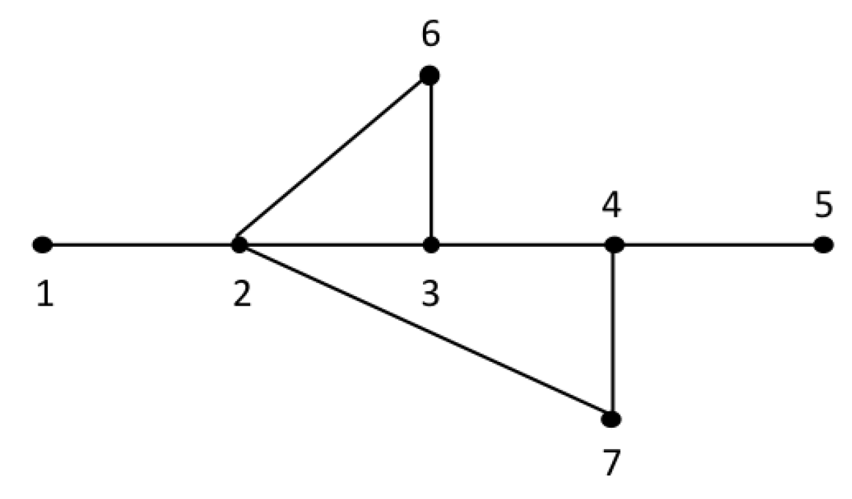
Grouping uncertain buses. After grouping adjacent uncertain buses, three groups and subnetworks are formed. However, these three subnetworks have overlapping buses. Hence, these subnetworks are merged into one larger subnetwork, as illustrated in Figure 4. The overlapping buses are buses 6 and 28. The blue box indicates the merged subnetwork. There are ten nodes in this subnetwork, and only six of them are candidate locations.

(5)

Minimizing the number of PMU for this subnetwork using Equation (9) gives the minimum number of PMU needed for this subnetwork as 3.

(6)

Maximizing the SORI for this subnetwork. There are six candidate buses in this subnetwork. The previous step yields the minimum number of PMU in this subnetwork as three. Therefore, there are 20 possible combinations of candidate locations. After examining the observability and SORI of the subnetwork, four optimal placements are identified.

(7)

Obtaining the optimal placements for this network by following the sub-steps below. The results are given in Table 1. According to Table 1, it is clear that:

Table 1. Phasor measurement unit (PMU) placement for 33 node test feeder using proposed hybrid method.

System	Min. No.	Location for Placing PMUS	SORI
IEEE 33	11	2, 8, 11, 14, 17, 21, 24, 32, 4, 26, 29	34
		2, 8, 11, 14, 17, 21, 24, 32, 5, 26, 29
		2, 8, 11, 14, 17, 21, 24, 32, 5, 27, 29
		2, 8, 11, 14, 17, 21, 24, 32, 5, 27, 30

(a)

at least 11 PMUs are required so as to make IEEE 33 node test feeder observable.

(b)

in order to maximize SORI, these 11 PMUs should be placed as follows:

• 8 PMUs will be assigned to the primary buses: 2, 8, 11, 14, 17, 21, 24, 32.
• The remaining 3 PMUs are assigned to uncertain buses: 4, 5, 26, 27, 29, 30. There are four optimal placements that can achieve the maximum SORI and full observability of the subnetwork: 5, 27, 30; 5, 27, 29; 5, 26, 29; 4, 26, 29;

4.2. IEEE 34 Node Test Feeder

The proposed hybrid method was then applied to IEEE 34 bus system [19,20]. The following steps illustrate how to implement our proposed method.

(1)

Minimizing the number of PMUs. Applying Equation (4) yielded the minimum number of PMU required to make the system observable as 12, that is, ${\mathit{f}}^{\mathit{T}}\mathit{x}=12$.

(2)

Maximizing the SORI obtained multiple solutions. In this step, Equation (5) was optimized with the coefficient in Equations (6) and (7). This step yielded 68 solutions, but some of them were identical. There were two distinct solutions among the 68 solutions, and the rest were the same.

(3)

Classifying the network buses based on the two solutions obtained from the previous step.

• Primary buses: 2, 4, 10, 12, 17, 21, 23, 25, 28, 31, 33.
• Uncertain buses: 7, 8.
• Trivial buses: 1, 3, 5, 6, 9, 11, 13, 14, 15, 16, 18, 19, 20, 22, 24, 26, 27, 29, 30, 32, 34.

(4)

Grouping uncertain buses. As there was only one group, hence only one subnetwork was formed. It consisted of these nodes: 6, 7, 8, 9.

(5)

Minimizing the number of PMUs for this subnetwork using Equation (9) gave the minimum number of PMU needed for this subnetwork which equals to one.

(6)

Maximizing the SORI for this subnetwork. It was found that two placement strategies can render the subnetwork observable and maximize the measurement redundancy.

(7)

In summary, the optimal placements for this network can be obtained following the sub-steps below. The results are tabulated in Table 2 and more information could be obtained as follows:

Table 2. PMU placement for 34 node test feeder using proposed hybrid method.

System	Min. No.	Location for Placing PMUs	SORI
IEEE 34	12	2, 4, 7, 10, 12, 17, 21, 23, 25, 28, 31, 33	42
		2, 4, 8, 10, 12, 17, 21, 23, 25, 28, 31, 33

(a)

At least 12 PMUs were needed to make the network observable.

(b)

In order to achieve maximized SORI, these 12 PMUs should be placed as follows:

• 11 PMUs should be assigned to the primary buses.
• 1 PMU should be assigned to bus 7 or 8.

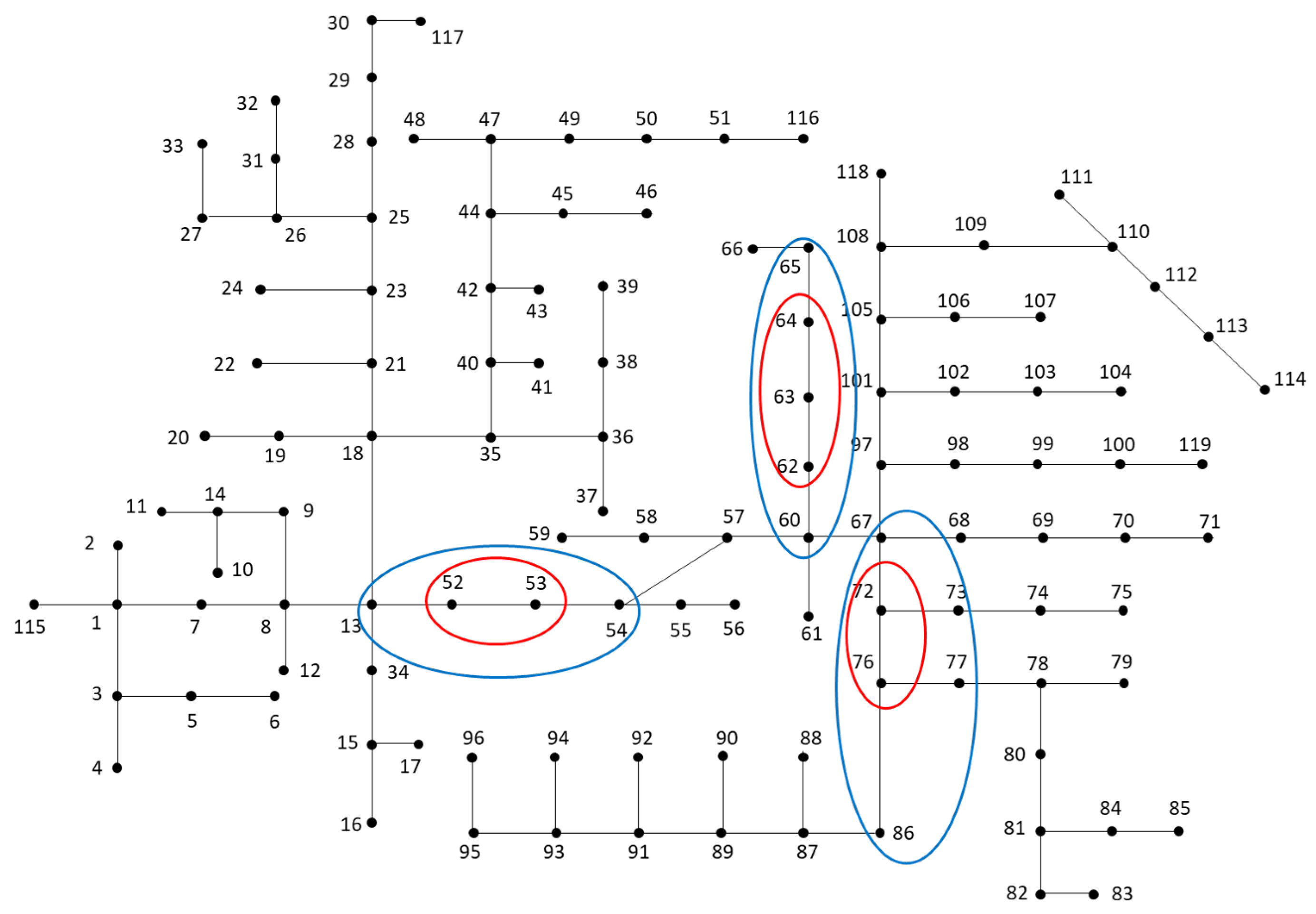
4.3. IEEE 123 Node Test Feeder

In order to verify the efficiency of our proposed method, a larger scale system, the IEEE 123 node test feeder is used [19,20]. This feeder consists of 123 nodes and several switches. There are 119 nodes in this network and the topology is illustrated in Figure 5.

Figure 5. IEEE 123 node test feeder.

(1)

Minimizing the number of PMUs. Note that at least 45 PMUs are needed to make the entire system observable.

(2)

Generate the $2n$ (in this case $2n=238$) solutions, out of which there are 5 distinct solutions and the rest are identical.

(3)

Classifying of the buses yields the following (the bus number is ignored for simplicity).

• Primary buses: 42 buses.
• Uncertain buses: 7 buses.
• Trivial buses: the rest of the buses (60 buses).

(4)

Grouping the uncertain nodes. There are three independent groups for this network and hence there are three subnetworks.

(5)

Optimization for each subnetwork. The minimum number of PMUs and placements that maximize SORI are tabulated in Table 3.

Table 3. Optimization results for each subnetwork.

Grouping	Minimum No. of PMU	Solutions that Maximize SORI
52, 53	1	52 or 53
62, 63, 64	1	62 or 63 or 64
72, 76	1	72 or 76

(6)

In summary, the optimal placements for this network can be obtained following the sub-steps below. In total there are 12 optimal placements that achieve minimum number of PMU and maximum SORI.

(a)

At least 45 PMUs are needed to make the network observable.

(b)

In order to achieve maximized SORI, these 45 PMUs should be placed as follows:

• 42 PMUs will be assigned to the primary buses (the bus number are not listed for simplicity).
• 1 PMU will be assigned to any bus between: 52, 53.
• 1 PMU will be assigned to any bus among: 62, 63, 64.
• 1 PMU will be assigned to any bus between: 72, 76.

4.4. Optimization Results Considering Single PMU Loss

When taking single PMU loss into consideration, a high number of PMUs is expected. Table 4 compares the minimum number of PMU required in different cases. The number of PMUs increases more than 2 times even when a single PMU loss occurs. The conclusion mentioned above is verified.

Table 4. Number of PMU required in different situations.

System	IEEE 33	IEEE 34	IEEE 123
Normal	11	12	45
Single PMU loss	24	27	97

The optimal solutions for the IEEE 34 node test feeder is given in Table 5. The optimal solutions for IEEE 33 and 123 node test feeder are too many to be exhaustively listed, so the placement strategies are summarized in Table 6 and Table 7 instead.

Table 5. PMU placement for 34 node test feeder using proposed hybrid method considering single PMU loss.

System	Min. No.	Location for Placing PMUs
IEEE 34	27	1,2,4,5,9,10,12,13,14,17,18,20,21,22,23,24, 25,28,29,31,32,33,34;15,26,6,7
		1,2,4,5,9,10,12,13,14,17,18,20,21,22,23,24, 25,28,29,31,32,33,34;15,26,6,8
		1,2,4,5,9,10,12,13,14,17,18,20,21,22,23,24, 25,28,29,31,32,33,34;15,26,7,8
		1,2,4,5,9,10,12,13,14,17,18,20,21,22,23,24, 25,28,29,31,32,33,34;15,27,6,7
		1,2,4,5,9,10,12,13,14,17,18,20,21,22,23,24, 25,28,29,31,32,33,34;15,27,6,8
		1,2,4,5,9,10,12,13,14,17,18,20,21,22,23,24, 25,28,29,31,32,33,34;15,27,7,8
		1,2,4,5,9,10,12,13,14,17,18,20,21,22,23,24, 25,28,29,31,32,33,34;16,26,6,7
		1,2,4,5,9,10,12,13,14,17,18,20,21,22,23,24, 25,28,29,31,32,33,34;16,26,6,8
		1,2,4,5,9,10,12,13,14,17,18,20,21,22,23,24, 25,28,29,31,32,33,34;16,26,7,8
		1,2,4,5,9,10,12,13,14,17,18,20,21,22,23,24, 25,28,29,31,32,33,34;16,27,6,7
		1,2,4,5,9,10,12,13,14,17,18,20,21,22,23,24, 25,28,29,31,32,33,34;16,27,6,8
		1,2,4,5,9,10,12,13,14,17,18,20,21,22,23,24, 25,28,29,31,32,33,34;16,27,7,8

Table 6. PMU placement for 33 node test feeder using proposed hybrid method considering single PMU loss.

Bus Type	Index	Bus Number	No. of Combination
Primary buses	-	1,2,3,6,8,10,12,14,16,17,18, 21,22,24,25,32,33	-
Groups	1	19,20	2
	2	4,5,26,27,28,29,30,31	9

Table 7. PMU placement for 123 node test feeder using proposed hybrid method considering single PMU loss.

Bus Type	Index	Bus Number	No. of Combination
Primary buses		1,2,3,4,5,6,8,10,11,12,13,14,15,16,17,19,20,
		21,22,23,24,25,27,30,31,32,33,34,37,38,39,
		40,41,42,43,45,46,47,48,51,54,55,56,58,59,
	-	60,61,65,66,67,70,71,72,74,75,76,78,79,81,	-
		82,83,84,85,87,88,89,90,91,92,93,94,95,96,
		97,100,101,103,104,106,107,108,110,111,
		113,114,115,116,117,118,119
Groups	1	52, 53	2
	2	28, 29	2
	3	49, 50	2
	4	62, 63, 64	3
	5	68, 69	2
	6	98, 99	2

4.5. Optimization Results without Considering Single PMU Loss

The optimal placements without considering PMU loss for the test systems are summarized in Table 8. The objectives of the optimization consist of minimum number of PMUs and maximum SORI. The proposed hybrid ILP-based method was able to find 2, 4, and 12 optimal placements for IEEE 34, 33 and 123 bus system respectively. It was confirmed that the results were the same with those obtained using the exhaustive search method. Therefore, it is concluded that the proposed hybrid ILP based method is able to identify all the alternative optimal solutions as the exhaustive search method does.

Table 8. Simulation results obtained for the IEEE 34, 33 and IEEE 123 systems without considering PMU loss.

Systems	Min. No. of PMU	Max. SORI	No. of Subnetworks	No. of Optimal Placements
		with Min. PMU
IEEE 34	12	42	1	2
IEEE 33	11	34	1	4
IEEE 123	45	162	3	12

The computational time of the proposed method is given in Table 9 and is compared with the ILP and the exhaustive search methods [21]. In the three test systems mentioned above, the ILP takes least time to find a optimal solution. However, the limitation of this method could not be ignored because it provides only one optimal solution. In practice some buses are not suitable or quite difficult to be installed with PMU due to hostile environment. Even though the customized exhaustive search method identifies all the optimal solutions, it takes more than 3 h for the IEEE 123 bus system. The consuming time would grow exponentially with the increasing scale of distribution system. The proposed hybrid ILP based method is able to give the same results as the customized exhaustive search method while it consumes much less time in the IEEE 123 bus system.

Table 9. Computational time comparison using three different method.

Systems	Custom. Exhaustive		ILP		Proposed Hybrid Method
	NO. of Solutions	Time	No. of Solutions	Time	No. of Solutions	Time
IEEE 34	2	0.26s	1	0.09s	2	3.61s
IEEE 33	4	62.13s	1	0.09s	4	3.54s
IEEE 123	12	> 3 hours	1	0.15s	12	12.77s

The proposed method includes the efficiency of the ILP algorithm and the ability of exhaustive search method to locate all the optimal solutions. Author response: please delete above sentence. The proposed method has dual advantage of being able to find all solutions to the optimization problem and being computationally efficient at the same time. The ILP based method makes it easy to be implemented and PMU loss can be integrated with less effort. With all optimal solutions obtained, the decision maker would evaluate these solutions using other criteria that are mathematically difficult to express or based on the application requirement to choose the best solution [14].

5. Conclusions

In this paper, a hybrid ILP method is proposed to find all the optimal solutions in the placement of PMUs. The constraints considered in the optimization include the system observability, number of PMUs and the measurement redundancy. A novel method is introduced to classify the network buses into three categories, and the uncertain buses are further analyzed and grouped. It is proven that the proposed method will not omit any optimal solutions that satisfy the given constraints. PMU loss can also be accounted for by the proposed method. The proposed method has been tested on the IEEE 33, 34 and 123 node test feeders, and the results show that the proposed method is able to give all the alternative solutions efficiently, even for large scale systems.

Appendix A.1. Proof of Δ Does Not Affect the Optimal Solutions of OPP

In this section it is proven mathematically that the optimal solutions, ${\mathit{x}}^{\mathbf{1}},{\mathit{x}}^{\mathbf{2}},\cdots ,{\mathit{x}}^{\mathbf{2}\mathit{n}}$, obtained using the modified coefficient $\overline{\mathit{g}}$ are also optimal solutions to the original optimization problem, with $0<\Delta <1$. The objective value of the original optimization problem is ${\mathit{g}}^T{\mathit{x}}^0$, where ${\mathit{x}}^0$ is the optimal solution obtained using the original coefficient $\mathit{g}$. Let $\overline{\mathit{x}}$ be the optimal solution corresponding to $\overline{\mathit{g}}$.

Since ${\mathit{x}}^0$ and $\overline{\mathit{x}}$ are the optimal solutions corresponding to $\mathit{g}$ and $\overline{\mathit{g}}$, the following inequalities can be deduced.

$$\begin{array}{cc}{\mathit{g}}^T{\mathit{x}}^0\hfill & \hfill \ge {\mathit{g}}^T\overline{\mathit{x}}\\ {\overline{\mathit{g}}}^T\overline{\mathit{x}}\hfill & \hfill \ge {\overline{\mathit{g}}}^T{\mathit{x}}^0.\end{array}$$

(A1)

The proof is completed by contradiction. Suppose the solution $\overline{\mathit{x}}$ is not the optimal solution to the original problem, it is deduced that ${\mathit{g}}^T\overline{\mathit{x}}<{\mathit{g}}^T{\mathit{x}}^0$ considering Equation (A1). Since $g_i\in \mathbb{N},x_i\in 0,1$, $\exists z\in \mathbb{Z}\mathrm{and}z>0$ such that

$${\mathit{g}}^T\overline{\mathit{x}}+z={\mathit{g}}^T{\mathit{x}}^0.$$

(A2)

Appendix A.1.1. When the Disturbance Is Positive

When $\Delta$ is added to one entry of $\mathit{g}$, $\overline{\mathit{g}}$ is constructed as:

$$\overline{\mathit{g}}={[g_1,\dots ,g_i+\Delta \dots ,g_n]}^T.$$

(A3)

So the following equation holds.

$${\overline{\mathit{g}}}^T{\mathit{x}}^0={\mathit{g}}^T{\mathit{x}}^0+\Delta x_i\ge {\mathit{g}}^T{\mathit{x}}^0.$$

(A4)

Combining inequalities Equations (A1) and (A4) yields

$${\overline{\mathit{g}}}^T\overline{\mathit{x}}\ge {\overline{\mathit{g}}}^T{\mathit{x}}^0\ge {\mathit{g}}^T{\mathit{x}}^0\ge {\mathit{g}}^T\overline{\mathit{x}}.$$

(A5)

Substitute Equation (A2) into Equation (A5), Equation (A6) can be deduced.

$${\overline{\mathit{g}}}^T\overline{\mathit{x}}\ge {\mathit{g}}^T\overline{\mathit{x}}+z.$$

(A6)

On the other hand, the construction of $\overline{\mathit{g}}$ implies that

$${\overline{\mathit{g}}}^T\overline{\mathit{x}}=[g_1,\dots ,g_i+\Delta \dots ,g_n]\mathit{x}={\mathit{g}}^T\overline{\mathit{x}}+\Delta x_i.$$

(A7)

From Equations (A6) and (A7) the following inequalities are deduced.

$$\begin{array}{c}{\overline{\mathit{g}}}^T\overline{\mathit{x}}-{\mathit{g}}^T\overline{\mathit{x}}\ge z\end{array}$$

(A8)

$$\begin{array}{c}{\overline{\mathit{g}}}^T\overline{\mathit{x}}-{\mathit{g}}^T\overline{\mathit{x}}\le \Delta .\end{array}$$

(A9)

Obviously the above inequalities cannot be true at the same time. Therefore, the assumption is wrong that solution $\overline{\mathit{x}}$ is not the optimal solution to the original problem.

Appendix A.1.2. When the Disturbance Is Negative

The construction of $\overline{\mathit{g}}$ is like

$$\overline{\mathit{g}}={[g_1,\dots ,g_i-\Delta \dots ,g_n]}^T.$$

(A10)

So the following equation holds.

$${\overline{\mathit{g}}}^T\overline{\mathit{x}}={\mathit{g}}^T\overline{\mathit{x}}-\Delta x_i\le {\mathit{g}}^T\overline{\mathit{x}}.$$

(A11)

Combining inequalities Equations (A1) and (A11) yields

$${\mathit{g}}^T{\mathit{x}}^0\ge {\mathit{g}}^T\overline{\mathit{x}}\ge {\overline{\mathit{g}}}^T\overline{\mathit{x}}\ge {\overline{\mathit{g}}}^T{\mathit{x}}^0.$$

(A12)

Substitute Equation (A2) into Equation (A12), Equation (A13) can be deduced.

$${\mathit{g}}^T\overline{\mathit{x}}+z\ge {\overline{\mathit{g}}}^T\overline{\mathit{x}}.$$

(A13)

On the other hand, the construction of $\overline{\mathit{g}}$ implies that

$${\overline{\mathit{g}}}^T\overline{\mathit{x}}=[g_1,\dots ,g_i-\Delta \dots ,g_n]\mathit{x}={\mathit{g}}^T\overline{\mathit{x}}-\Delta x_i.$$

(A14)

From Equations (A13) and (A14) the following inequalities are deduced.

$$\begin{array}{c}{\mathit{g}}^T\overline{\mathit{x}}-{\overline{\mathit{g}}}^T\overline{\mathit{x}}\ge z\hfill \\ {\mathit{g}}^T\overline{\mathit{x}}-{\overline{\mathit{g}}}^T\overline{\mathit{x}}\le \Delta .\hfill \end{array}$$

(A15)

Obviously the above inequaitons cannot be true at the same time. Therefore, the assumption is wrong that solution $\overline{\mathit{x}}$ is not the optimal solution to the original problem.

Hence, with $0<\Delta <1$, the optimal solutions obtained using the modified coefficient $\overline{\mathit{g}}$ are definitely the optimal solutions to the original problem.

Appendix A.2. Proof of Set γ = Γ,ξ = Ξ,λ = Λ

The authors have stated that the proposed hybrid method based on linear integer programming algorithm is able to find all the alternative optimal solutions that satisfy the constraints of achieving the minimum number of PMU and maximizing the SORI. The reasoning is that, on one hand, the classification of network buses is valid not only on multiple solutions, but also those potential missing optimal solutions, and on the other hand, the uncertain buses are grouped into independent groups and each group is optimized separately in an exhaustive manner. Therefore, it is guaranteed that no optimal alternative solution is omitted by our proposed method. In this section, it is proven that the classification of network buses also applies to potential missing optimal solutions, which is the most important assertion that underscores our proposed hybrid method.

Appendix A.2.1. Proof of γ = Γ

The proof is completed by contradiction that $\Gamma \subseteq \gamma$. Assume that a bus k is an element of set $\Gamma$ but not an element of set $\gamma$. That is to say among the $2n$ solutions, at least one of them is

$${\mathit{x}}^{\mathit{k}}={[\dots ,\dots ,x_k=0,\dots ]}^T$$

(A16)

Since all the $2n$ solutions are optimal solution, ${\mathit{x}}^{\mathit{k}}$ must be an optimal solution as well. Therefore, the bus k which equals to zero in one of the optimal solutions cannot be an element of $\Gamma$, which however, violates the assumption. Hence, it is impossible that the bus k is an elements of the set $\Gamma$, but not an element of the set $\gamma$, which therefore indicates that $\Gamma \subseteq \gamma$.

Next, it is proven similarly that $\gamma \subseteq \Gamma$, by contradiction. Assume that a bus k is an element of the set $\gamma$ but not an element of set $\Gamma$. This means that the bus k is assigned with a PMU in every solution among the $2n$ solutions but there is a missing optimal solution in which bus k is not assigned with a PMU. That is to say, there is at least one missing optimal solution with the following structure:

$$\overline{\mathit{x}}={[\dots ,\dots ,x_k=0,\dots ]}^T.$$

(A17)

However, note that $x_k$ is always assigned with a PMU (the value of this entry is 1) in all the $2n$ solutions. The following ${\overline{\mathit{g}}}^{\mathit{n}+\mathit{k}}$ is used when generating the multiple solutions,

$${\overline{\mathit{g}}}^{\mathbf{n}+\mathit{k}}={[g_1,g_2,\dots ,g_k-\Delta ,\dots ,g_n]}^T.$$

(A18)

The associated solution, which is one of the $2n$ solutions, is

$${\overline{\mathit{x}}}^{\mathbf{n}+\mathit{k}}={[\dots ,\dots ,x_k=1,\dots ]}^T$$

(A19)

Since both $\overline{\mathit{x}}$ and ${\overline{\mathit{x}}}^{\mathit{n}+\mathit{k}}$ are the optimal solutions, they ought to share the same objective function value.

$${\mathit{g}}^T{\overline{\mathit{x}}}^{\mathbf{n}+\mathit{k}}={\mathit{g}}^T\overline{\mathit{x}}$$

(A20)

Note that the only differences between ${\overline{\mathit{g}}}^{\mathit{n}+\mathit{k}}$ and $\mathit{g}$ are their i-th elements, and the i-th element of ${\overline{\mathit{g}}}^{\mathit{n}+\mathit{k}}$ is $\Delta$ smaller than that of $\mathit{g}$. Since the i-th element of ${\overline{\mathit{x}}}^{\mathit{n}+\mathit{k}}$ is 0, the value of ${\mathit{g}}^T\overline{\mathit{x}}={{\overline{\mathit{g}}}^{\mathit{n}+\mathit{k}}}^T\overline{\mathit{x}}$. Furthermore, since the i-th element of ${\overline{\mathit{x}}}^{\mathit{n}+\mathit{k}}$ is 1, ${\left\{{\overline{\mathit{g}}}^{\mathit{n}+\mathit{k}}\right\}}^T{\overline{\mathit{x}}}^{\mathit{n}+\mathit{k}}<{\mathit{g}}^T{\overline{\mathit{x}}}^{\mathit{n}+\mathit{k}}$.

$$\begin{array}{ccc}\hfill {\mathit{g}}^T\overline{\mathit{x}}& =& {\left\{{\overline{\mathit{g}}}^{\mathbf{n}+\mathit{k}}\right\}}^T\overline{\mathit{x}}\hfill \end{array}$$

(A21)

$$\begin{array}{ccc}\hfill {\mathit{g}}^T{\overline{\mathit{x}}}^{\mathbf{n}+\mathit{k}}& >& {\left\{{\overline{\mathit{g}}}^{\mathbf{n}+\mathit{k}}\right\}}^T{\overline{\mathit{x}}}^{\mathbf{n}+\mathit{k}}\hfill \end{array}$$

(A22)

Using Equations (A20)–(A22), it is deduced that

$${\left\{{\overline{\mathit{g}}}^{\mathbf{n}+\mathit{k}}\right\}}^T\overline{\mathit{x}}>{\left\{{\overline{\mathit{g}}}^{\mathbf{n}+\mathit{k}}\right\}}^T{\overline{\mathit{x}}}^{\mathbf{n}+\mathit{k}}$$

(A23)

Note that ${\overline{\mathit{x}}}^{\mathit{n}+\mathit{k}}$ in Equation (A23) is obtained by maximizing the ${\left\{{\overline{\mathit{g}}}^{\mathit{n}+\mathit{k}}\right\}}^T\mathit{x}$ in Equation (5). Therefore, $\overline{\mathit{x}}$ does not exist such that Equation (A23) holds. That is, it is impossible that a bus k is an element of set $\gamma$ but not an element of set $\Gamma$, which means $\gamma \subseteq \Gamma$.

In conclusion, it is proven that $\gamma =\Gamma$. This is to say, if a bus is assigned with a PMU in every solution among the $2n$ solutions, it will surely be assigned with a PMU in any potential missing optimal solutions.

Appendix A.2.2. Proof of ξ = Ξ

It can be proven by contradiction that $\Xi \subseteq \xi$. Assume that a bus k is an element of set $\Xi$ but not an element of set $\xi$. That is to say, among the $2n$ solutions, at least one of them is

$${\mathit{x}}^{\mathit{k}}={[\dots ,\dots ,x_k=1,\dots ]}^T.$$

(A24)

Since all the $2n$ solutions are optimal solutions, ${\mathit{x}}^{\mathit{k}}$ must be an optimal solution as well. Therefore, the bus k which equals to 1 in one of the optimal solutions cannot be an element of $\Xi$, which thus violates the assumption. Hence, it is impossible that the bus k is an elements of the set $\Xi$ but not an element of the set $\xi$, which indicates that $\Xi \subseteq \xi$.

It is proven that $\xi \subseteq \Xi$ by contradiction. Assume that a bus k is an element of the set $\xi$ but not an element of the set $\Xi$, which means the bus k is not assigned with a PMU in any of those $2n$ solutions, but assigned with a PMU in a missing optimal solution. That is to say, there is at least one missing optimal solution of the following structure:

$$\overline{\mathit{x}}={[\dots ,\dots ,x_k=1,\dots ]}^T.$$

(A25)

However, in all the $2n$ solutions, the $x_k$ is always assigned with 0. In one of the $2n$ solutions, the following $\overline{{\mathit{g}}^{\mathit{k}}}$ is used.

$${\overline{\mathit{g}}}^{\mathit{k}}={[g_1,g_2,\dots ,g_k+\Delta ,\dots ,g_n]}^T$$

(A26)

The associated solution, which is one of the $2n$ solutions, is

$${\overline{\mathit{x}}}^{\mathit{k}}={[\dots ,\dots ,x_k=0,\dots ]}^T.$$

(A27)

Since both $\overline{\mathit{x}}$ and ${\overline{\mathit{x}}}^{\mathit{k}}$ are optimal solutions, they ought to share the same objective function value.

$${\mathit{g}}^T{\overline{\mathit{x}}}^{\mathit{k}}={\mathit{g}}^T\overline{\mathit{x}}.$$

(A28)

Note that the only differences of ${\overline{\mathit{g}}}^{\mathit{k}}$ and $\mathit{g}$ are their i-th elements, the i-th element of ${\overline{\mathit{g}}}^{\mathit{k}}$ is $\Delta$ greater than that of $\mathit{g}$. Since the i-th element of ${\overline{\mathit{x}}}^{\mathit{k}}$ is 1, the value of ${\mathit{g}}^T\overline{\mathit{x}}<{\left\{{\overline{\mathit{g}}}^{\mathit{k}}\right\}}^T\overline{\mathit{x}}$. Since the i-th element of ${\overline{\mathit{x}}}^{\mathit{k}}$ is 0, ${\left\{{\overline{\mathit{g}}}^{\mathit{k}}\right\}}^T{\overline{\mathit{x}}}^{\mathit{k}}={\mathit{g}}^T{\overline{\mathit{x}}}^{\mathit{k}}$.

$$\begin{array}{ccc}\hfill {\mathit{g}}^T\overline{\mathit{x}}& <& {\left\{{\overline{\mathit{g}}}^{\mathit{k}}\right\}}^T\overline{\mathit{x}}\hfill \end{array}$$

(A29)

$$\begin{array}{ccc}\hfill {\mathit{g}}^{\prime }{\overline{\mathit{x}}}^{\mathit{k}}& =& {\left\{{\overline{\mathit{g}}}^{\mathit{k}}\right\}}^T{\overline{\mathit{x}}}^{\mathit{k}}.\hfill \end{array}$$

(A30)

Using Equations (A28)–(A30),

$${\left\{{\overline{\mathit{g}}}^{\mathit{k}}\right\}}^T\overline{\mathit{x}}>{\left\{{\overline{\mathit{g}}}^{\mathit{k}}\right\}}^T{\overline{\mathit{x}}}^{\mathit{k}}.$$

(A31)

Note that ${\overline{\mathit{x}}}^{\mathit{k}}$ in Equation (A31) is obtained by maximizing ${\left\{{\overline{\mathit{g}}}^{\mathit{k}}\right\}}^T\mathit{x}$ in Equation (5). Therefore, $\overline{\mathit{x}}$ does not exist such that Equation (A31) holds. That is, it is impossible that a bus k is an element of the set $\xi$ but not an element of the set $\Xi$, which means $\xi \subseteq \Xi$.

In conclusion, it is proven that $\xi =\Xi$. This is to say, if a bus is never assigned with a PMU in any solution among the $2n$ solutions, it will not be assigned with a PMU in any potential missing optimal solution.

Appendix A.2.3. Proof of λ = Λ

Since $\gamma =\Gamma$ and $\xi =\Xi$, the conclusion that $\lambda =\Lambda$ can be drawn without much effort. Therefore, since these three sets are identical, and each subnetwork is searched in an exhaustive manner, it is ascertained that no one optimal solution is missing. Therefore, the proposed hybrid method generates the same solutions to OPP problem with the exhaustive search method.

References

1. Baldwin, T.L.; Mili, L.; Boisen, M.B.; Adapa, R. Power system observability with minimal phasor measurement placement. IEEE Trans. Power Syst. 1993, 8, 707–715. [Google Scholar] [CrossRef]
2. Manousakis, N.M.; Korres, G.N.; Georgilakis, P.S. Taxonomy of PMU placement methodologies. IEEE Trans. Power Syst. 2012, 27, 1070–1077. [Google Scholar] [CrossRef]
3. Xu, B.; Abur, A. Observability analysis and measurement placement for systems with PMUs. In Proceedings of the IEEE PES Power Systems Conference and Exposition, New York, NY, USA, 10–13 October 2004; Volume 2, pp. 943–946. [Google Scholar]
4. Chakrabarti, S.; Kyriakides, E. Optimal placement of phasor measurement units for power system observability. IEEE Trans. Power Syst. 2008, 23, 1433–1440. [Google Scholar] [CrossRef]
5. Chakrabarti, S.; Kyriakides, E.; Eliades, D.G. Placement of synchronized measurements for power system observability. IEEE Trans. Power Deliv. 2009, 24, 12–19. [Google Scholar] [CrossRef]
6. Milošević, B.; Begović, M. Nondominated sorting genetic algorithm for optimal phasor measurement placement. IEEE Trans. Power Syst. 2003, 18, 69–75. [Google Scholar] [CrossRef]
7. Nuqui, R.F.; Phadke, A.G. Phasor measurement unit placement techniques for complete and incomplete observability. IEEE Trans. Power Deliv. 2005, 20, 2381–2388. [Google Scholar] [CrossRef]
8. Yuill, W.; Edwards, A.; Chowdhury, S.; Chowdhury, S. Optimal PMU placement: A comprehensive literature review. In Proceedings of the 2011 IEEE Power and Energy Society General Meeting, San Diego, CA, USA, 24–29 July 2011; pp. 1–8. [Google Scholar]
9. Manousakis, N.; Korres, G.; Georgilakis, P. Optimal placement of phasor measurement units: A literature review. In Proceedings of the 2011 16th International Conference on Intelligent System Applications to Power Systems, Hersonissos, Greece, 25–28 September 2011; pp. 1–6. [Google Scholar]
10. Sodhi, R.; Srivastava, S.; Singh, S. Optimal PMU placement to ensure system observability under contingencies. In Proceedings of the Power Energy Society General Meeting, Calgary, AB, Canada, 26–30 July 2009; pp. 1–6. [Google Scholar]
11. Gou, B. Generalized integer linear programming formulation for optimal PMU placement. IEEE Trans. Power Syst. 2008, 23, 1099–1104. [Google Scholar] [CrossRef]
12. Gou, B. Optimal placement of PMUs by integer linear programming. IEEE Trans. Power Syst. 2008, 23, 1525–1526. [Google Scholar] [CrossRef]
13. Dua, D.; Dambhare, S.; Gajbhiye, R.K.; Soman, S.A. Optimal Multistage Scheduling of PMU Placement: An ILP Approach. IEEE Trans. Power Deliv. 2008, 23, 1812–1820. [Google Scholar] [CrossRef]
14. Sun, L.; Chen, T.; Chen, X.; Ho, W.K.; Ling, K.; Tseng, K.; Amaratunga, G.A.J. Optimum Placement of Phasor Measurement Units in Power Systems. IEEE Trans. Instrum. Meas. 2019, 68, 421–429. [Google Scholar] [CrossRef]
15. Xia, N.; Gooi, H.B.; Chen, S.; Wang, M. Redundancy based PMU placement in state estimation. Sustain. Energy Grids Netw. 2015, 2, 23–31. [Google Scholar] [CrossRef]
16. Maji, T.K.; Acharjee, P. Multiple solutions of optimal PMU placement using exponential binary PSO algorithm for smart grid applications. IEEE Trans. Ind. Appl. 2017, 53, 2550–2559. [Google Scholar] [CrossRef]
17. Zhong, J. Phasor measurement unit (PMU) placement optimisation in power transmission network based on hybrid approach. Master’s Thesis, Electrical and Computer Engineering, RMIT University, Melbourne, Australia, 2012. [Google Scholar]
18. Zhu, J. Optimal reconfiguration of electrical distribution network using the refined genetic algorithm. Electr. Power Syst. Res. 2002, 62, 37–42. [Google Scholar] [CrossRef]
19. Kersting, W.H. Radial distribution test feeders. IEEE Trans. Power Syst. 1991, 6, 975–985. [Google Scholar] [CrossRef]
20. Kersting, W. Radial distribution test feeders. In Proceedings of the 2001 IEEE Power Engineering Society Winter Meeting. Conference Proceedings (Cat. No. 01CH37194), Columbus, OH, USA, 28 January–1 February 2001; Volume 2, pp. 908–912. [Google Scholar]
21. Chen, X.; Chen, T.; Tseng, K.; Sun, Y.; Amaratunga, G. Hybrid approach based on global search algorithm for optimal placement of Micro-PMU in distribution networks. In Proceedings of the 2016 IEEE Innovative Smart Grid Technologies—Asia (ISGT-Asia), Melbourne, Australia, 28 November–1 December 2016; pp. 559–563. [Google Scholar]
Article Metrics
Citations
Article Access Statistics
Multiple requests from the same IP address are counted as one view.