Nonlinear Control for Autonomous Trajectory Tracking While Considering Collision Avoidance of UAVs Based on Geometric Relations

Abstract

Trajectory tracking with collision avoidance for a multicopter is solved based on geometrical relations. In this paper, a new method is proposed for a multicopter to move from the start position to a desired destination and track a pre-planned trajectory, while avoiding collisions with obstacles. The controller consists of two parts: First, a tracking control is introduced based on the errors between the relative position of the multicopter and the reference path. Second, once the obstacles with a high possibility of collision are detected, a boundary sphere/cylinder of the obstacle is generated by the dimensions of the vehicle and the obstacles, so as to define the safety and risk areas. Afterwards, from the relation between the vehicle’s motion direction, and the tangential lines from the vehicle’s current position to the sphere/cylinder of the obstacle, a collision detection angle is computed to decide the fastest direction to take in order to avoid a collision. The obstacle/collision avoidance control is activated locally when an object is close, and null if the vehicle moves away from the obstacles. The velocity control law and the guidance law are obtained from the Lyapunov stability. In addition, a proportional controller is used at the end of vehicle’s journey to ensure the vehicle stops at the target position. A numerical simulation in different scenarios was performed to prove the effectiveness of the proposed algorithm.

1. Introduction

Today, multicopters are being used more frequently due to the their many practical applications, especially in places where the working environment is dangerous or human capacity is limited, such as data collection [1,2], search and rescue [3], payload carrying [4], crop spraying in agriculture [5,6,7], and military operations [8,9]. In these applications, the multicopters usually have to work within a complex environment. Furthermore, the problem of avoiding collisions between a multicopter and a variety of moving objects or stationary objects is extremely important in autonomous flight. This is especially true in some applications that require the combination of trajectory tracking with collision avoidance, such as crop spraying in agriculture, which requires the multicopter to move from the start position to a desired destination point and track a pre-planned trajectory with a reference speed, while avoiding collisions with obstacles. In this case, the coordination between the tracking control and the collision avoidance control must be harmonized to ensure that the vehicle operates safely and efficiently. This problem is especially difficult and represents a significant challenge in the autonomous flight of the vehicle. Much research has been conducted in related fields. Generally, the literature can be classified into two main groups. In the first group, the research is based on a proposed navigation algorithm, which integrates the movement of the unmanned aerial vehicles (UAVs) from the start position to a given point with collision avoidance, but they do not focus on the trajectory tracking of the vehicle. In the second group, these studies introduce methods for trajectory tracking or target tracking of the UAVs with an object, but they do not consider collision avoidance.

1.1. Related Works

Collision avoidance of UAVs is a classic research area in the field of robotics. The challenge is that the vehicle must share space with other objects, which may be moving or stationary. Therefore, the vehicle has to be integrated with a reliable sensing system to estimate the position of the objects and generate safe areas to move within, so as to avoid a collision. Furthermore, the sensing system may encounter errors, which can be caused by time delay, wind, or other disturbances. Therefore, the collision avoidance algorithm must compensate for these uncertainties and low computations. There are many studies based on vision systems to detect and avoid obstacles based on the optical flow sensor [10,11,12,13,14,15,16], or stereo vision, monocular camera [17,18,19,20,21,22,23]. Most of these studies only focused on the image processing techniques with intensive computation. Other studies, using various techniques, have been inspired by the path-planning algorithm to solve the collision avoidance problem for UAVs [24,25,26,27,28,29,30,31]. These proposed methods are based on optimization techniques. Therefore, the computation is complicated. In order to overcome this disadvantage, other more simple and low computation methods for collision avoidance of UAVs have been proposed that are based on a geometry approach [32,33,34,35,36,37,38]. However, the fundamental limitation of these solutions is that they focus on avoiding obstacles or collisions without considering a method to approach the desired position or to track a pre-planned trajectory before and after the completion of the collision avoidance process.

Another challenge is the tracking control of UAVs, which has become a popular topic in recent years. There are many studies that attempt to solve this problem. Various control methodologies have been proposed, such as: Nonlinear model predictive control [39,40,41], nonlinear robust adaptive control [42,43], and simultaneous localization and mapping (SLAM) [44,45]. Other research has focused on the sliding mode control (SMC) [46,47,48,49,50,51]. Most of these studies, however, only focus on trajectory tracking or tracking a moving object.

A few papers have studied the much more complicated case of combining both tracking control and obstacle/collision avoidance control [52,53]. In these studies, the procedure to obtain controllers is not a simple one, making it difficult to implement in real world applications. Therefore, a simple and practical solution in both tracking control and collision avoidance control is a necessary requirement to guarantee the safe, flexible, and efficient operation of the vehicle.

1.2. Main Contributions

The combination of trajectory tracking control and obstacle/collision avoidance control in the autonomous flights of multicopters is introduced in this paper. This study presents a new method to drive the multicopters from a start position to a desired destination, whilst tracking a pre-planned trajectory and avoiding collisions with obstacles. The problem becomes simplified if the control objective is divided into two tasks, which are tracking control and collision avoidance control. Both of these were solved separately, and then combined by the movement strategy. The main advantage of this combination is to ensure that each controller focuses on one task. Furthermore, the collision avoidance control method can only work locally, and it is null if the vehicle moves away from the obstacles. Following this, the tracking control continues working without perturbations. This makes computation much faster. First, from the geometrical relation between a multicopter and the pre-planned path, the tracking errors are computed to design a tracking control law that guarantees the vehicle follows the reference path with a reference speed. Once an obstacle is detected, the safety and risk zones are generated, and then a collision detection angle is computed to determine the fastest direction for avoiding obstacles. A guidance law is presented to control the heading angle of the multicopter to steer the vehicle to the left or right to avoid an object. The overall control laws are obtained from the Lyapunov stability. During the working process, both the velocity and heading angular rate are simultaneously controlled to ensure a smooth movement of the vehicle. In addition, the proportional (P) controller is used in the end of the robot’s journey to guarantee the vehicle reaches a given point and stops there.

Furthermore, this study presents a simple, practical, and effective controller in comparison with other advanced methods [54,55] with considerations of the implementation on a real-time embedded system. The full control scheme, introduced in this paper, comprises of a multi-loop architecture, which includes an outer loop and an inner loop. The presented algorithms are applied in the outer loop position and heading control to generate a set-point for velocity and heading angular rate. A conventional proportional integral derivative (PID) controller is applied in the inner loop. The performance of the proposed algorithms is verified by numerical simulations with a quadcopter.

1.3. The Organizations

The remainder of this article is organized as follows. Section 2 describes the mathematic model of a quadcopter, which is used for the simulation. In Section 3, the trajectory tracking control, based on the geometrical relations, is presented. In Section 4, the collision avoidance control and movement strategy are introduced. The numerical simulations with different scenarios are given in Section 5. Finally, brief conclusions and further work are discussed in Section 6.

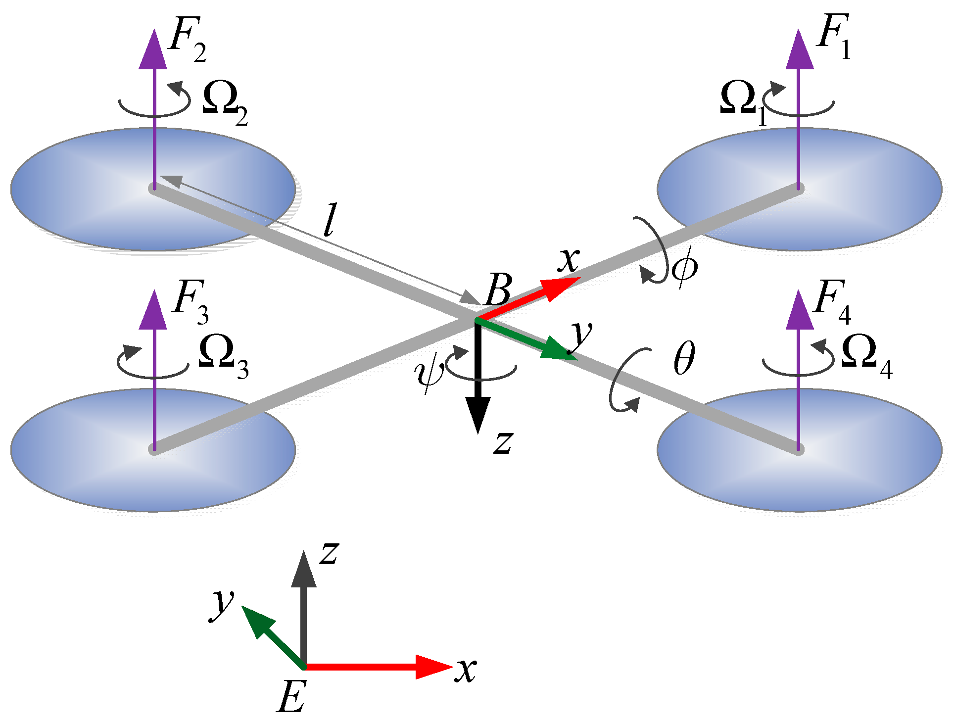
2. Mathematic Model of a Quadcopter

The dynamic model of a quadcopter has been reported in many related studies [56,57,58,59,60,61,62,63,64,65,66,67]. In this section, the mathematic model is briefly presented. The fixed frame, E, and body frame, B, are considered and presented in Figure 1.

Let ${\varphi }_m,{\theta }_m$, ${\varphi }_m\in \left(-\pi /2,\pi /2\right), {\theta }_m\in \left(-\pi /2,\pi /2\right)$ and ${\psi }_m$, ${\psi }_m\in \left(-\pi ,\pi \right)$ represent roll, pitch, and yaw angles of a quadcopter, respectively. The position of vehicle in a fixed frame E is denoted by vector $\left(x_m,y_m,z_m\right)$. l represents the arm length of the vehicle. Let $I_{xx},I_{yy},I_{zz}$ represent the moment of inertia along x, y, z axes of the quadcopter, respectively; m is the total mass. The mathematic model of the vehicle is described as follows [60]:

$$\left[\begin{array}{l}{\ddot{\varphi }}_m\\ {\ddot{\theta }}_m\\ {\ddot{\psi }}_m\\ {\ddot{z}}_m\\ {\ddot{x}}_m\\ {\ddot{y}}_m\end{array}\right]=\left[\begin{array}{c}\frac{I_{yy}-I_{zz}}{I_{xx}}{\dot{\theta }}_m{\dot{\psi }}_m+\frac{l}{I_{xx}}{U}_2\\ \frac{I_{zz}-I_{xx}}{I_{yy}}{\dot{\varphi }}_m{\dot{\psi }}_m+\frac{l}{I_{yy}}{U}_3\\ \frac{I_{xx}-I_{yy}}{I_{zz}}{\dot{\theta }}_m{\dot{\varphi }}_m+\frac{1}{I_{zz}}{U}_4\\ \frac{\left(\cos {\varphi }_m\cos {\theta }_m\right)U_1}{m}-g\\ \frac{U_1}{m}\left(\cos {\varphi }_m\sin {\theta }_m\cos {\psi }_m+\sin {\varphi }_m\sin {\psi }_m\right)\\ \frac{U_1}{m}\left(\cos {\varphi }_m\sin {\theta }_m\sin {\psi }_m-\sin {\varphi }_m\cos {\psi }_m\right)\end{array}\right]$$

(1)

where, the first three equations of expression (1) describe the rotational dynamics, and the next three equations present the translational dynamics; $U_i\in ℝ, i=1,2,3,4$ are control inputs to control the thrust, roll, pitch, and yaw rotation of the vehicle, which are given by [60]:

$$\left[\begin{array}{l}{U}_1\\ U_2\\ U_3\\ U_4\end{array}\right]=\left[\begin{array}{c}b\left({\mathsf{\Omega }}_1^2+{\mathsf{\Omega }}_2^2+{\mathsf{\Omega }}_3^2+{\mathsf{\Omega }}_4^2\right)\\ b\left(-{\mathsf{\Omega }}_2^2+{\mathsf{\Omega }}_4^2\right)\\ b\left(-{\mathsf{\Omega }}_1^2+{\mathsf{\Omega }}_3^2\right)\\ d\left({\mathsf{\Omega }}_1^2-{\mathsf{\Omega }}_2^2+{\mathsf{\Omega }}_3^2-{\mathsf{\Omega }}_4^2\right)\end{array}\right]$$

(2)

where F_i = bΩ_i represents the thrust force produced by the motor i (i = 1, …, 4); Ω_i denotes the speed of the motor i; b and d represent the thrust coefficient and ratio coefficient from force to torque, respectively. The mathematic model of quadcopter UAVs, as shown in Equations (1) and (2), is used to verify the proposed algorithm. Let $u_x$ and $u_y$ are position controllers of x, and y axes, which can be obtained from the Equation (1).

$$\{\begin{array}{l}{u}_x=\left(\cos {\varphi }_m\sin {\theta }_m\cos {\psi }_m+\sin {\varphi }_m\sin {\psi }_m\right)\\ u_y=\left(\cos {\varphi }_m\sin {\theta }_m\sin {\psi }_m-\sin {\varphi }_m\cos {\psi }_m\right)\end{array}$$

(3)

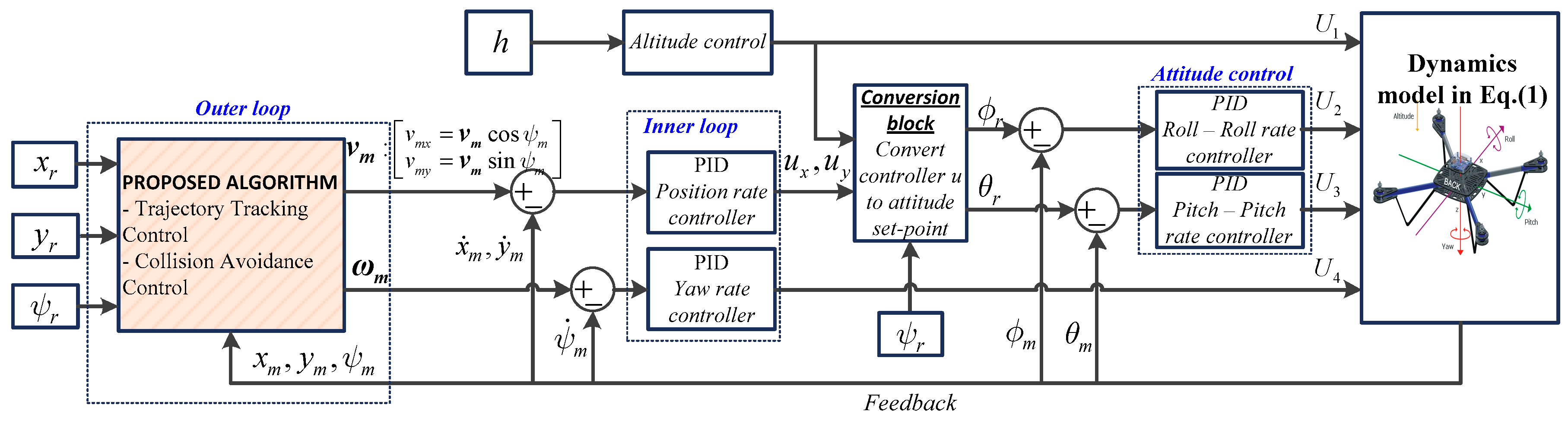
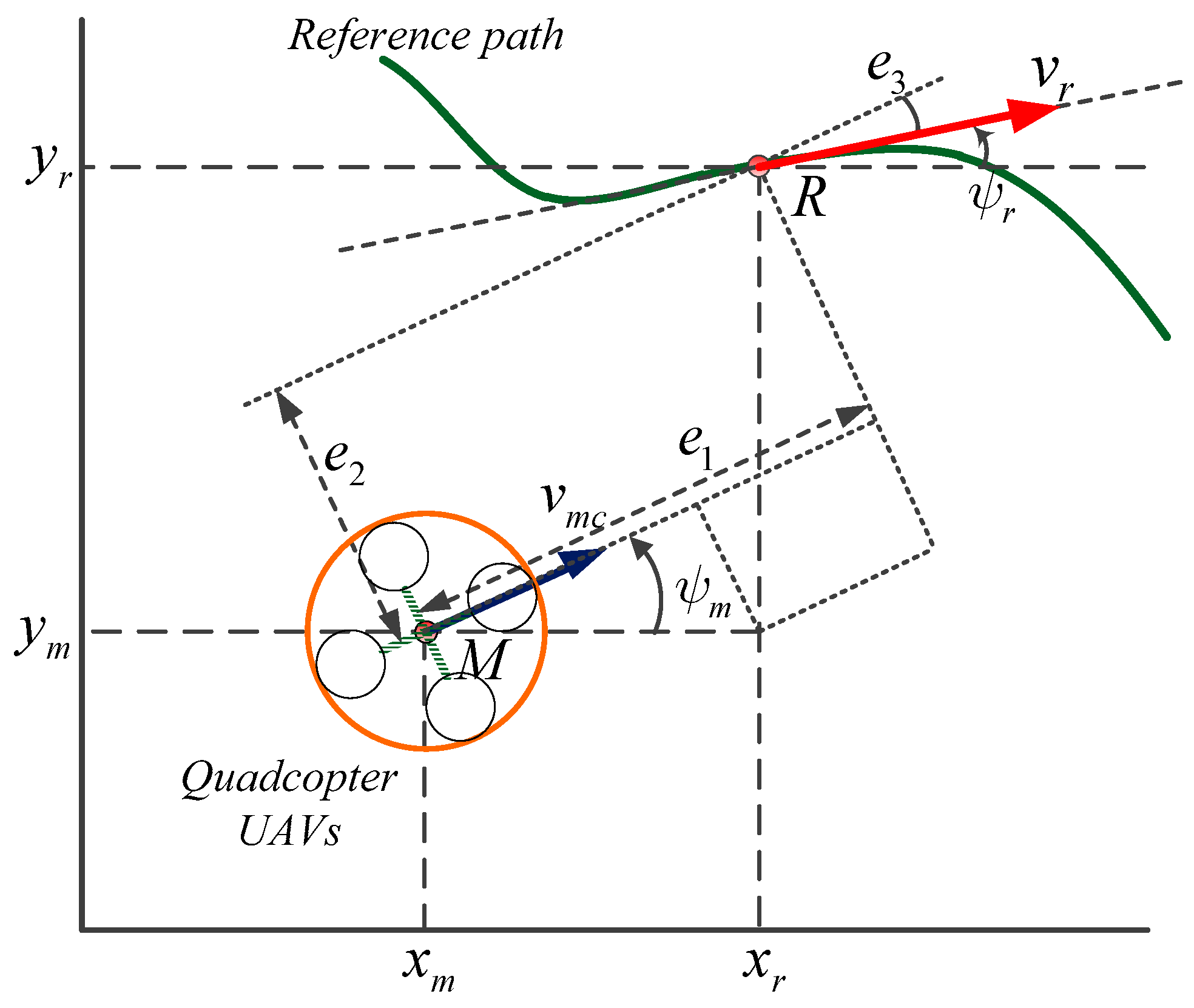
3. Trajectory Tracking Control

This section introduces the trajectory tracking control algorithm. The objective of trajectory tracking is to drive the convergence of errors between the vehicle’s position and a time-varying reference point of the pre-planned trajectory to zero. From Equation (3), it can be seen that [62,63]:

$$\begin{array}{l}{\varphi }_r={\sin }^{-1}\left(u_x\sin {\psi }_r-u_y\cos {\psi }_r\right)\\ {\theta }_r={\sin }^{-1}\left(\frac{u_x\cos {\psi }_r+u_y\sin {\psi }_r}{\cos {\varphi }_r}\right)\end{array}$$

(4)

Obviously, Equation (4) is used to convert the position controllers ($u_x,u_y$) into desired reference attitude angles ${\varphi }_r,{\theta }_r$ via desired yaw (${\psi }_r$). The values of ${\varphi }_r,{\theta }_r$ are considered as set-points of attitude controller for rotational dynamics in Equation (1). In addition, the position controllers $u_x,u_y$ are indirectly generated from the velocity, which comes from the trajectory tracking controller. Furthermore, in this study, we only consider that the mission of a quadcopter is to track a pre-planned trajectory when the vehicle is stably operating at a constant altitude h. Therefore, the problem becomes a trajectory tracking control in two dimensions with x and y axes. It means that the velocity of the vehicle with dynamics model in Equation (1) can also be computed from Figure 2 [64,65]. The equation form of velocity can be derived by:

$$\left[\begin{array}{l}{\dot{x}}_m\\ {\dot{y}}_m\\ {\dot{\psi }}_m\end{array}\right]=\left[\begin{array}{cc}\cos {\psi }_m& 0\\ \sin {\psi }_m& 0\\ 0& 1\end{array}\right]\left[\begin{array}{c}{v}_m\\ {\omega }_m\end{array}\right]$$

(5)

where $v_m, {\omega }_m$ denote the velocity and heading angular rate of the quadcopter, respectively.

Let $R\left(x_r,y_r\right)$, $v_r$ denote the reference point and the movement velocity of it on the reference path, respectively; ${\psi }_r, {\omega }_r$ represent the orientation angle (desired yaw of quadcopter) and the orientation’s angular rate (desired heading angular rate of quadcopter) of the reference velocity, respectively. The movement equation of reference point can be derived as follows:

$$\left[\begin{array}{l}{\dot{x}}_r\\ {\dot{y}}_r\\ {\dot{\psi }}_r\end{array}\right]=\left[\begin{array}{cc}\cos {\psi }_r& 0\\ \sin {\psi }_r& 0\\ 0& 1\end{array}\right]\left[\begin{array}{c}{v}_r\\ {\omega }_r\end{array}\right]$$

(6)

Let $e_1, e_2, e_3$ denote the position tracking errors as shown in Figure 2. Its values can be obtained by:

$$\left[\begin{array}{l}{e}_1\\ e_2\\ e_3\end{array}\right]=\left[\begin{array}{ccc}\cos {\psi }_m& \sin {\psi }_m& 0\\ -\sin {\psi }_m& \cos {\psi }_m& 0\\ 0& 0& 1\end{array}\right]\left[\begin{array}{c}{x}_r-x_m\\ y_r-y_m\\ {\psi }_r-{\psi }_m\end{array}\right]$$

(7)

Theorem 1.

The position tracking error,$e_i (i=1,2,3)$, converges to zero if the velocity$v_m$and heading angular rate${\omega }_m$satisfy the controller in Equation (8).

$$\{\begin{array}{l}{v}_m=v_r\cos e_3+k_1{e}_1\\ {\omega }_m={\omega }_{tracking}\end{array}$$

(8)

$where{\omega }_{tracking}={\omega }_r+\frac{v_r}{k_2}{e}_2+\frac{k_3}{k_2}\sin e_3$, $k_1, k_2, k_3>0$.

Proof. 

From Equation (7), the derivative of $e_1, e_2, e_3$ is computed as follows:

$$\oplus {\dot{e}}_1=\left({\dot{x}}_r-{\dot{x}}_m\right)\cos {\psi }_m-{\dot{\psi }}_m\sin {\psi }_m\left(x_r-x_m\right)+\left({\dot{y}}_r-{\dot{y}}_m\right)\sin {\psi }_m+{\dot{\psi }}_m\cos {\psi }_m\left(y_r-y_m\right)$$

Substituting Equations (5) and (6) to ${\dot{e}}_1$

$$\begin{array}{cc}\hfill {\dot{e}}_1=& \left(v_r\cos {\psi }_r-v_m\cos {\psi }_m\right)\cos {\psi }_m+\left(v_r\sin {\psi }_r-v_m\sin {\psi }_m\right)\sin {\psi }_m\hfill \\ \hfill & -{\dot{\psi }}_m\left[\left(x_r-x_m\right)\sin {\psi }_m-\left(y_r-y_m\right)\cos {\psi }_m\right]\hfill \\ \hfill =& v_r\left(\cos {\psi }_r\cos {\psi }_m+\sin {\psi }_r\sin {\psi }_m\right)-v_m\left(\cos {\psi }_m\cos {\psi }_m+\sin {\psi }_m\sin {\psi }_m\right)\hfill \\ \hfill & +{\dot{\psi }}_m\left[-\left(x_r-x_m\right)\sin {\psi }_m+\left(y_r-y_m\right)\cos {\psi }_m\right]\hfill \\ \hfill =& v_r\cos \left({\psi }_r-{\psi }_m\right)-v_m+{\dot{\psi }}_m{e}_2\hfill \\ \hfill =& v_r\cos e_3-v_m+{\omega }_m{e}_2\hfill \end{array}$$

$$\oplus {\dot{e}}_2=-\left({\dot{x}}_r-{\dot{x}}_m\right)\sin {\psi }_m-{\dot{\psi }}_m\cos {\psi }_m\left(x_r-x_m\right)+\left({\dot{y}}_r-{\dot{y}}_m\right)\cos {\psi }_m-{\dot{\psi }}_m\sin {\psi }_m\left(y_r-y_m\right)$$

Substituting Equations (5) and (6) to ${\dot{e}}_2$

$$\begin{array}{cc}\hfill {\dot{e}}_2=& -\left(v_r\cos {\psi }_r-v_m\cos {\psi }_m\right)\sin {\psi }_m+\left(v_r\sin {\psi }_r-v_m\sin {\psi }_m\right)\cos {\psi }_m\hfill \\ \hfill & -{\dot{\psi }}_m\left[\left(x_r-x_m\right)\cos {\psi }_m+\left(y_r-y_m\right)\sin {\psi }_m\right]\hfill \\ \hfill =& v_r\left(\sin {\psi }_r\cos {\psi }_m-\cos {\psi }_r\sin {\psi }_m\right)+v_m\left(\cos {\psi }_m\sin {\psi }_m-\sin {\psi }_m\cos {\psi }_m\right)\hfill \\ \hfill & -{\dot{\psi }}_m\left[\left(x_r-x_m\right)\cos {\psi }_m+\left(y_r-y_m\right)\sin {\psi }_m\right]\hfill \\ \hfill =& v_r\sin \left({\psi }_r-{\psi }_m\right)-{\dot{\psi }}_m{e}_1\hfill \\ \hfill =& v_r\sin e_3-{\omega }_m{e}_1\hfill \end{array}$$

$$\begin{array}{cc}\hfill \oplus {\dot{e}}_3& ={\dot{\psi }}_r-{\dot{\psi }}_m\hfill \\ \hfill & ={\omega }_r-{\omega }_m\hfill \end{array}$$

Considering the Lyapunov function candidate:

$$V_0=\frac{1}{2}{e}_1^2+\frac{1}{2}{e}_2^2+k_2\left(1-\cos e_3\right),k_2>0$$

The derivative of $V_0$ is obtained as follows:

$$\begin{array}{cc}\hfill {\dot{V}}_0& =e_1{\dot{e}}_1+e_2{\dot{e}}_2+k_2{\dot{e}}_3\sin e_3\hfill \\ \hfill & =e_1\left(v_r\cos e_3-v_m+{\omega }_m{e}_2\right)+e_2\left(v_r\sin e_3-{\omega }_m{e}_1\right)+k_2\left({\omega }_r-{\omega }_m\right)\sin e_3\hfill \\ \hfill & =e_1\left(v_r\cos e_3-v_m\right)+k_2\sin e_3\left({\omega }_r-{\omega }_m+\frac{v_r{e}_2}{k_2}\right)\hfill \end{array}$$

To achieve a negative value of ${\dot{V}}_0$, the tracking controller, $\left(v_m,{\omega }_m\right)$, is chosen as Equation (8). □

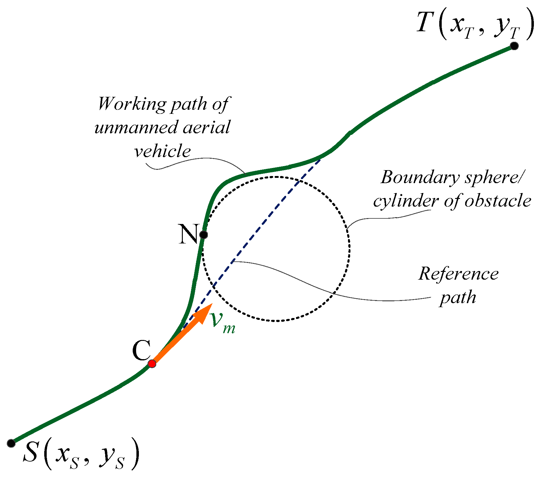
4. Collision Avoidance Control and Movement Strategy

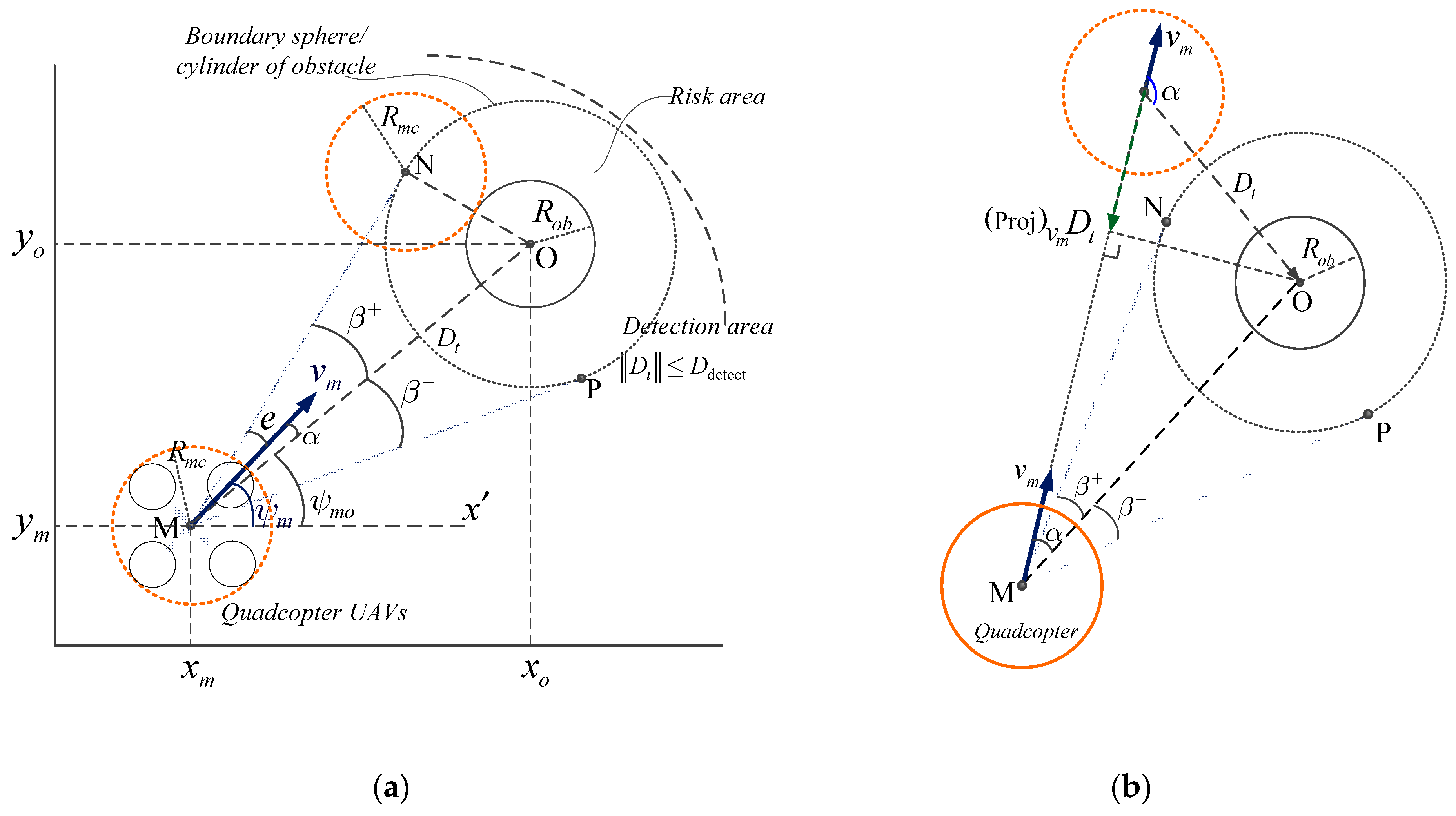
4.1. Statement Problem

Safe and stable operations are critically important issues for executing the tasks of an autonomous vehicle. A controller for collision avoidance is presented in this section. The goal of the control law is to generate the flight path through the safety zone and among obstacles. First, several important definitions, which are based on the geometrical relations, are presented as follows (Figure 3a):

Definition 1.

The obstacle detection. An obstacle is detected if the relative distance $D_t$ satisfies the following expression:

$$\Vert D_t\Vert \le D_{\mathrm{detect}}$$

(9)

where$D_{\mathrm{detect}}$represents the detection distance of the sensor;$D_t$denotes the relative distance between the vehicle and an obstacle. Let $O\left(x_o,y_o\right)$ denote a stationary position of an obstacle in the Cartesian coordinate. The value of $D_t$ and its derivative can be computed as follows:

$$\Vert D_t\Vert =\Vert \overrightarrow{MO}\Vert =\sqrt{{\left(x_o-x_m\right)}^2+{\left(y_o-y_m\right)}^2}$$

(10)

$$\Vert {\dot{D}}_t\Vert =-\frac{{\dot{x}}_m\left(x_o-x_m\right)+{\dot{y}}_m\left(y_o-y_m\right)}{\Vert D_t\Vert }$$

(11)

Definition 2.

The risk area. Once an obstacle is detected, a boundary sphere/cylinder of the obstacle is generated to define a risk area, as shown in Figure 3a. The radius of the boundary is computed as follows:

$$R=R_{safe}+R_{ob}$$

(12)

where$R_{ob}$denotes the dimension of the obstacle.$R_{safe}$and $R_{mc}$ represent the safety radius and the real radius of the vehicle, which includes the propellers, respectively.

$$R_{safe}\ge R_{mc}$$

(13)

In order to easily compute and design a controller, let us consider that $R_{safe}=R_{mc}$.

Definition 3.

Collision. A collision occurs between the quadcopter and an obstacle if the relative distance $D_t$ satisfies the following expression:

$$\Vert D_t\Vert <R$$

(14)

Definition 4.

Collision detection and the avoidance direction. Let${\beta }^{+}$and${\beta }^{-}$$(0<{\beta }^{+}<\pi /2$, $-\pi /2< {\beta }^{-}<0)$ represent the angles of the vectors $\overrightarrow{MN}$ and $\overrightarrow{MP}$ with the vector $D_t$, respectively.

$${\beta }^{\pm }=\pm {\sin }^{-1}\left(\frac{R}{\Vert D_t\Vert }\right)$$

(15)

Collision detection. A collision will occur when the orientation of the velocity vector $v_m$ is in the collision cone NMP, meaning that the heading angle ${\psi }_m$ satisfies the following conditions:

$$\angle PM{x}^{\prime }<{\psi }_m<\angle NM{x}^{\prime }\iff {\psi }_{mo}+{\beta }^{-}<{\psi }_m<{\psi }_{mo}+{\beta }^{+}$$

(16)

The avoidance direction. Let$\alpha$denotethe collision detection angle, $\alpha =\left(v_m, D_t\right)$.

$$\alpha ={\psi }_m-{\psi }_{mo}$$

(17)

where

$${\psi }_{mo}={\tan }^{-1}\left(\frac{y_o-y_m}{x_o-x_m}\right)$$

(18)

The avoidance direction of the vehicle is determined based on angle $\alpha$. From Equations (16) and (17), it is easy to see that: If $0\le \alpha <{\beta }^{+}\iff {\psi }_{mo}\le {\psi }_m<{\psi }_{mo}+{\beta }^{+}$, meaning that the orientation of velocity $v_m$ is in $\angle NMO$. The fastest avoidance direction is the left side of the obstacle. Therefore, the vehicle turns left to avoid a collision, the collision detection angle $\alpha$ tracks ${\beta }^{+}$. Conversely, if ${\beta }^{-}<\alpha <0\iff {\psi }_{mo}+{\beta }^{-}<{\psi }_m<{\psi }_{mo}$, the orientation of velocity $v_m$ is in $\angle PMO$. The fastest avoidance direction is the right side of the obstacle. Therefore, the vehicle turns right to avoid a collision, $\alpha$ tracks ${\beta }^{-}$.

Definition 5.

The completion of collision avoidance. Let the vector projection of vector$D_t(D_t\ne 0)$onto vector$v_m\left(v_m\ne 0\right)$be given by Figure 3b:

$$\begin{array}{cc}\hfill {\left(\mathrm{Proj}\right)}_{v_m}{D}_t& =\sigma v_m\hfill \\ \hfill & =\frac{\Vert D_t\Vert \Vert v_m\Vert \cos \alpha }{{\Vert v_m\Vert }^2}{v}_m\hfill \end{array}$$

(19)

From Figure 3b and Equation (19), the collision avoidance is completely successful if $\cos \alpha <0$, meaning that, angle $\alpha$ satisfies the following expression:

$$[\begin{array}{l}\pi /2<\alpha <\pi \\ -\pi <\alpha <-\pi /2\end{array}$$

(20)

Obviously, at the time successful collision avoidance, the velocity vector $v_m$ is perpendicular to vector $D_t$, meaning that the angle $\alpha$ reaches $\pm \pi /2$, $(\alpha ={\beta }^{\pm }=\pm \pi /2)$.

Remark 1.

If angle $\alpha$ satisfies the following expression:

$$[\begin{array}{l}{\beta }^{+}\le \alpha <\pi /2\\ -\pi /2<\alpha \le {\beta }^{-}\end{array}$$

(21)

Then, the orientation of velocity $v_m$ is outside of the collision cone NMP, which is shown in Figure 3b. This means that the collision will not occur again. Therefore, collision avoidance is considered to be basically completed.

Remark 2.

As a result of Definitions 4 and 5 and Remark 1, the necessary conditions to activate the collision avoidance controller are given by:

$$[\begin{array}{l}0\le \alpha <{\beta }^{+}<\pi /2\\ -\pi /2<{\beta }^{-}<\alpha <0\end{array}$$

(22)

Definition 6.

Sufficient conditions to activate the collision avoidance control. Let $D_{active} \left(0<D_{active}\le D_{\mathrm{detect}}\right)$ represent the relative distance, at which the collision avoidance algorithm is activated, meaning that the controller will start to work if $D_t$ satisfies the following expression:

$$\Vert D_t\Vert \le D_{active}$$

(23)

From Remark 2 and Definition 6, the general conditions to activate the collision avoidance control are given by Equations (22) and (23).

4.2. Collision Avoidance Algorithm and Movement Strategy

4.2.1. Collision Avoidance Controller Design

The objective of the collision avoidance control is to require the angle $\alpha$ tracks ${\beta }^{\pm }$ until $\alpha \ge {\beta }^{+}$ or $\alpha \le {\beta }^{-}$, meaning that when the tracking error angle, $e={\beta }^{\pm }-\alpha$, converges to zero, the collision avoidance process is basically completed (Remark 1). The derivative of e is computed as follows:

$$\dot{e}={\dot{\beta }}^{\pm }-\dot{\alpha }$$

(24)

where ${\dot{\beta }}^{\pm }$ is obtained from Equation (15).

$${\dot{\beta }}^{\pm }=\frac{\pm 1}{\sqrt{1-{\left(\frac{R}{\Vert D_t\Vert }\right)}^2}}\left(\frac{-R\Vert {\dot{D}}_t\Vert }{{\Vert D_t\Vert }^2}\right)=\frac{\mp R}{\Vert D_t\Vert \sqrt{{\Vert D_t\Vert }^2-R^2}}\Vert {\dot{D}}_t\Vert$$

(25)

From Equations (5), (11), and (25), ${\dot{\beta }}^{\pm }$ can be re-written as follows:

$$\begin{array}{c}{\dot{\beta }}^{\pm }=\frac{\pm R{v}_m}{\Vert D_t\Vert \sqrt{{\Vert D_t\Vert }^2-R^2}}\left(\cos {\psi }_m\underset{\cos {\psi }_{mo}}{\underbrace{\frac{\left(x_o-x_m\right)}{\Vert D_t\Vert }}}+\sin {\psi }_m\underset{\sin {\psi }_{mo}}{\underbrace{\frac{\left(y_o-y_m\right)}{\Vert D_t\Vert }}}\right)\\ \iff {\dot{\beta }}^{\pm }=\frac{\pm R{v}_m}{\Vert D_t\Vert \sqrt{{\Vert D_t\Vert }^2-R^2}}\cos \alpha \end{array}$$

(26)

The derivative of $\alpha$ is computed from Equations (17) and (18) as follows:

$$\begin{array}{c}\begin{array}{cc}\hfill \dot{\alpha }& ={\dot{\psi }}_m-{\dot{\psi }}_{mo}\hfill \\ \hfill & ={\dot{\psi }}_m-\left[\frac{1}{{\left(\frac{y_o-y_m}{x_o-x_m}\right)}^2+1}\left(\frac{-{\dot{y}}_m\left(x_o-x_m\right)+{\dot{x}}_m\left(y_o-y_m\right)}{{\left(x_o-x_m\right)}^2}\right)\right]\hfill \end{array}\\ \iff \dot{\alpha }= {\dot{\psi }}_m-\frac{{\dot{x}}_m\left(y_o-y_m\right)-{\dot{y}}_m\left(x_o-x_m\right)}{{\left(x_o-x_m\right)}^2+{\left(y_o-y_m\right)}^2}\end{array}$$

(27)

From Equations (5), (10), and (27), $\dot{\alpha }$ can be re-written as follows:

$$\begin{array}{c}\dot{\alpha }={\omega }_m-\frac{1}{\Vert D_t\Vert }{v}_m\left(\cos {\psi }_m\underset{\sin {\psi }_{mo}}{\underbrace{\frac{\left(y_o-y_m\right)}{\Vert D_t\Vert }}}-\sin {\psi }_m\underset{\cos {\psi }_{mo}}{\underbrace{\frac{\left(x_o-x_m\right)}{\Vert D_t\Vert }}}\right)\\ \iff \dot{\alpha }={\omega }_m+\frac{1}{\Vert D_t\Vert }{v}_m\sin \alpha \end{array}$$

(28)

From Equations (24), (26), and (28), $\dot{e}$ can be obtained as follows:

$$\begin{array}{c}\begin{array}{cc}\hfill \dot{e}& =\frac{1}{\Vert D_t\Vert } \left(\underset{\tan {\beta }^{\pm }}{\underbrace{\frac{\pm R}{\sqrt{{\Vert D_t\Vert }^2-R^2}}}}\cos \alpha -\sin \alpha \right)v_m-{\omega }_m\hfill \\ \hfill & =\frac{1}{\Vert D_t\Vert } \left(\frac{\sin e}{\cos {\beta }^{\pm }}\right)v_m-{\omega }_m\hfill \end{array}\\ \iff \dot{e}=\left[\frac{\sin e}{\Vert D_t\Vert \cos {\beta }^{\pm }}-1\right]\left[\begin{array}{l}{v}_m\\ {\omega }_m\end{array}\right]\end{array}$$

(29)

It is easy to understand that $\dot{e}$ is always a continuous function when ${\beta }^{\pm }$ satisfies the Equation (22). Therefore, the controller $\left(v_m, {\omega }_m\right)$ to avoid a collision is obtained by the Theorem 2.

Theorem 2.

The tracking error angle e converges to zero, meaning that the collision avoidance process is basically completed, if the velocity$v_m$and heading angular rate ${\omega }_m$ satisfy Equation (30):

$$\{\begin{array}{l}{v}_m=v_r\cos e_3+k_1{e}_1\\ {\omega }_m={\omega }_{avoid}\end{array}$$

(30)

where ${\omega }_{avoid}=\frac{v_m\sin e+ke}{\Vert D_t\Vert \cos {\beta }^{\pm }}$, k is a positive value.

Proof. 

Considering the Lyapunov function candidate:

$$V_1=\frac{1}{2}{e}^2$$

The derivative of $V_1$ is computed as follows:

$$\begin{array}{cc}\hfill {\dot{V}}_1& =e\dot{e}\hfill \\ \hfill & =e\left(\frac{\sin e}{\Vert D_t\Vert \cos {\beta }^{\pm }}{v}_m-{\omega }_m\right)\hfill \end{array}$$

To achieve a negative value of ${\dot{V}}_1$, the collision avoidance controller, $\left(v_m,{\omega }_m\right)$, is chosen as Equation (30). □

4.2.2. Movement Strategy

In this section, the movement strategy of the vehicle with tracking control and collision avoidance control is presented. Let us assume that the vehicle moves from a start position $S\left(x_S, y_S\right)$ to a given point $T\left(x_T, y_T\right)$ and tracks a reference path. In the movement process, let $C\left(x_C, y_C\right)$ be the position at which both values of $\alpha$ and $D_t$ satisfy Equations (22) and (23), meaning that the collision avoidance algorithm is activated. Let $N\left(x_N, y_N\right)$ denote a position at which the collision avoidance is completed, meaning that values of $\alpha$ and $D_t$ do not satisfy conditions of Equations (22) and (23). The working path of the vehicle can be divided into two parts as shown in Figure 4.

Part 1: The curves SC, NT. The vehicle tracks the reference path with the velocity and heading angular rate, as shown in the tracking controller in Equation (8).

Part 2: The curve CN. This curve shows the working path of the vehicle in order to avoid an obstacle when a collision is detected. The collision avoidance algorithm is activated at point C and null at point N, as shown in the avoidance controller in Equation (30).

Method to approach the final destination T: When the vehicle closely approaches the desired position T, meaning that the relative distance $\xi =\sqrt{{\left(x_T-x_m\right)}^2+{\left(y_T-y_m\right)}^2}\le 2m$, the velocity must be decreased to stop the vehicle at this point. Therefore, the proportional controller for position (i.e., P controller) is applied to drive the vehicle towards the destination point and stop there as follows Equation (31).

$$v_m=\left[\begin{array}{c}{v}_{mx}\\ v_{my}\end{array}\right]=\left[\begin{array}{c}{K}_{Pos}\left(x_T-x_m\right)\\ K_{Pos}\left(y_T-y_m\right)\end{array}\right]$$

(31)

where $K_{Pos}$ is a positive value.

4.3. Stability Analysis

As previously mentioned, the collision avoidance control only works locally, when a collision is detected, and it is null if the vehicle moves away from the obstacles. Therefore, tracking control and collision avoidance control should be separately worked to ensure that each of controller’s highest focus is on the individual task. This means that at any given time, only one controller is activated, either the tracking control or the collision avoidance control. The condition of selection must follow Equations (22) and (23). A total Lyapunov function is considered as follows:

$$V=p{V}_0+q{V}_1$$

(32)

where $[\begin{array}{ll}p=1, q=0& if [\begin{array}{l}\alpha \notin \left({\beta }^{-}, 0\right)\cup \left[0, {\beta }^{+}\right)\\ \Vert D_t\Vert >D_{active}\end{array}\\ p=0, q=1& if\{\begin{array}{l}\alpha \in \left({\beta }^{-}, 0\right)\cup \left[0, {\beta }^{+}\right)\\ \Vert D_t\Vert \le D_{active}\end{array}\end{array}$.

Derivative of V is computed and proven as a negative value by Theorems 1 and 2.

$$\dot{V}=p{\dot{V}}_0+q{\dot{V}}_1$$

(33)

If: $[\begin{array}{l}\alpha \notin \left({\beta }^{-}, 0\right)\cup \left[0, {\beta }^{+}\right)\\ \Vert D_t\Vert >D_{active}\end{array}\Rightarrow \dot{V}={\dot{V}}_0<0 \iff \{\begin{array}{l}{v}_m=v_r\cos e_3+k_1{e}_1\\ {\omega }_m={\omega }_{tracking}={\omega }_r+\frac{v_r}{k_2}{e}_2+\frac{k_3}{k_2}\sin e_3\end{array}$

If: $\{\begin{array}{l}\alpha \in \left({\beta }^{-}, 0\right)\cup \left[0, {\beta }^{+}\right)\\ \Vert D_t\Vert \le D_{active}\end{array}\Rightarrow \dot{V}={\dot{V}}_1 <0\iff \{\begin{array}{l}{v}_m=v_r\cos e_3+k_1{e}_1\\ {\omega }_m={\omega }_{avoid}=\frac{v_m\sin e+ke}{\Vert D_t\Vert \cos {\beta }^{\pm }}\end{array}$

Hence, the stability of control system in both tracking control and collision avoidance control is guaranteed by Lyapunov criterion.

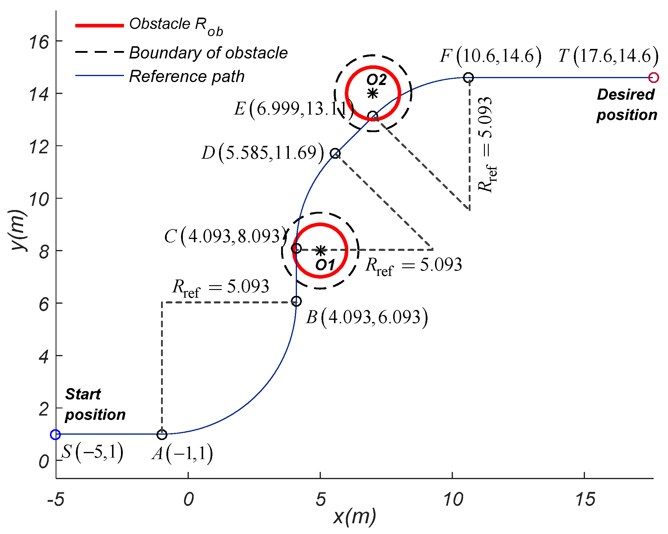
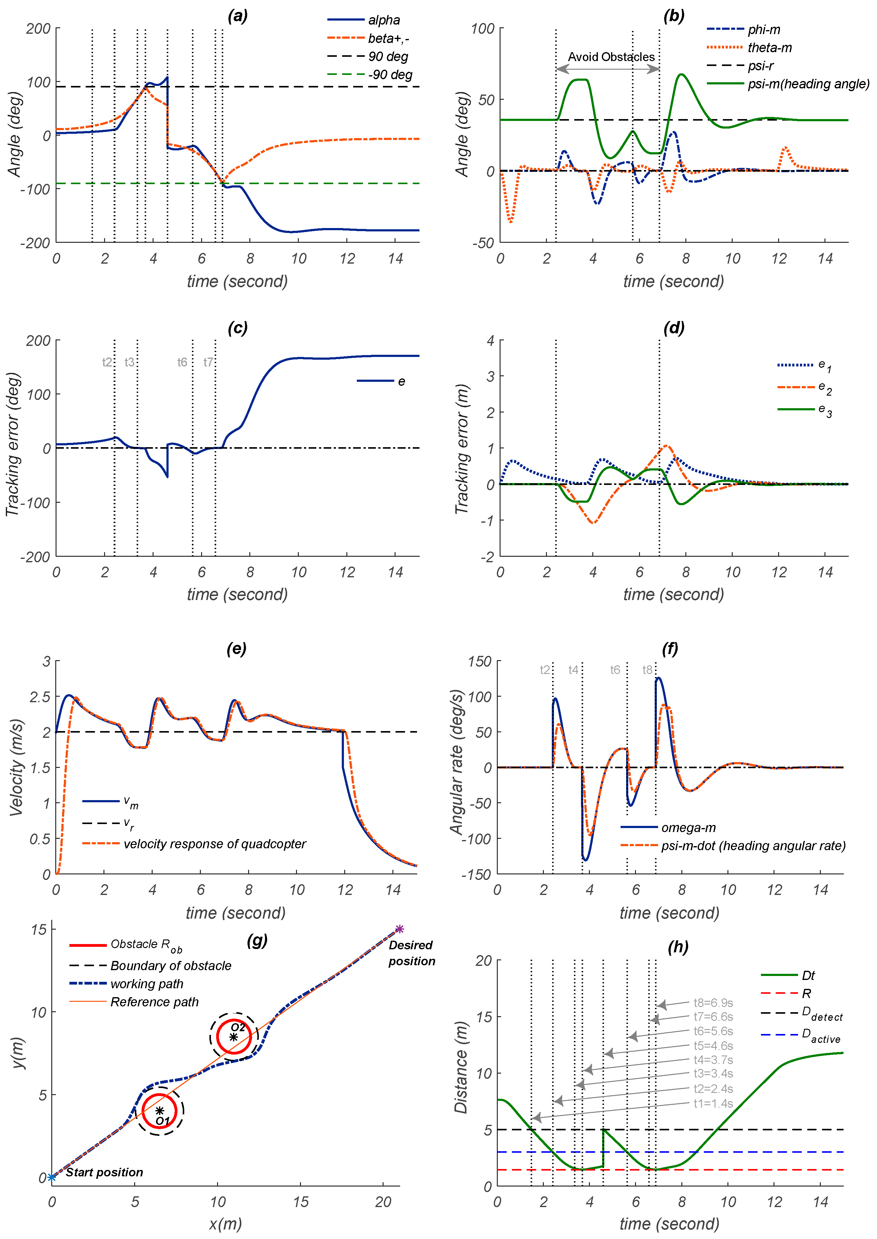
5. Simulation Results and Discussions

5.1. Simulation Assumptions

The numerical simulations were carried out based on the mathematic model in Equations (1) and (2) to verify the performance of the proposed method with a general control structure, as shown in Figure 5. Several assumptions for the simulation platform and working environment are given as follows: First, the system’s parameters of the quadcopter for the simulation are given in

Table 1. System’s parameters of quadcopter for simulation.

Symbol	Descriptions	Value and Unit
Rmc	Radius of quadcopter (including propeller)	0.35 m
m	Total mass of quadcopter	1.12 kg
Ixx	Moment of inertia along x-axis	0.0119 kg.m2
Iyy	Moment of inertia along y-axis	0.0119 kg.m2
Izz	Moment of inertia along z-axis	0.0223 kg.m2
g	Gravitational acceleration	9.81 N/m2
Rob	Radius of obstacle	1 m
b	Thrust coefficient	7.73213 (10−6)
d	Drag coefficient	1.27513 (10−7)
Ddetect	Detection radius of sensor	5 m
Dactive	Distance of activating the collision avoidance algorithm	3 m

. Second, the mission of a quadcopter is to track a pre-planned trajectory and avoid collisions when the vehicle is stably operating in a constant altitude h. Therefore, the simulation only considers the performance of vehicle in x and y axes. The quadcopter model and proposed algorithm are implemented and simulated in the MATLAB Simulink.

The simulation presents two examples. The first example is performed with a straight-line trajectory and other parameters of the simulation environment are shown in

Table 2. Parameters of the first example simulation.

Symbol	Descriptions	Value and Unit
S	Start position	(0, 0)
T	Desired position	T (21, 15)
vr	Reference velocity	2 m/s
wr	Reference angular rate	0 rad/s
O1,O2	Obstacle positions	O1 (6.5, 4), O2 (11, 8.5)
k1, k2, k3	Position tracking controller gains	0.8, 1.2, 1.8
k	Collision avoidance controller gain	10

. In the second example, the simulation is performed with a spline trajectory as shown in Figure 6, and other parameters are given in

Table 3. Parameters of the second example simulation.

Symbol	Descriptions	Value and Unit
S	Start position	(−5, 1)
T	Desired position	(17.6, 14.6)
vr	Reference velocity	2 m/s
wr	Reference angular rate in SA, BC, DE, FT (as Figure 6)	0 rad/s
	Reference angular rate in AB, CD, EF (as Figure 6)	$v_r/R_{ref}$ rad/s
O	Obstacle positions	O1 (5, 8), O2 (7, 14)
k1, k2, k3	Position tracking controller gains	0.5, 0.8, 2.8
k	Collision avoidance controller gain	10

.

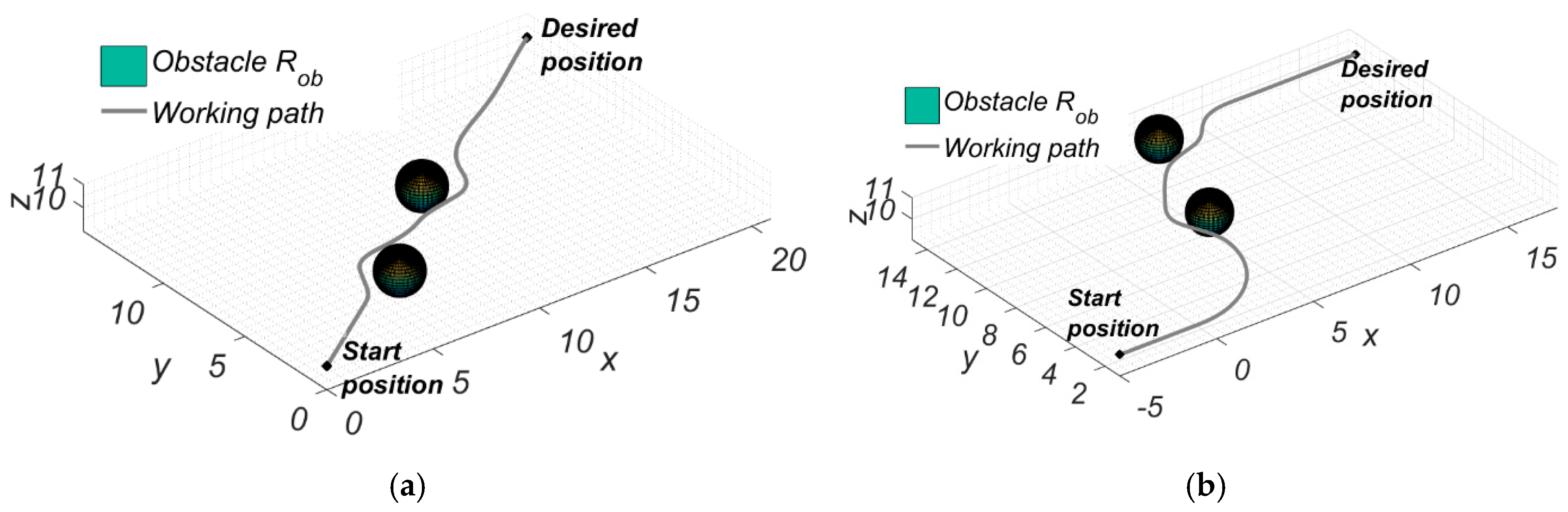
5.2. Simulation Results

Example 1: The reference path is a straight-line. In this section, the first simulation was performed with obstacles at positions: O1 (6.5, 4) and O2 (11, 8.5).

The results of the simulation are shown in Figure 7. As soon as the tracking control was activated $0<t<t_2=2.4\mathrm{s}$ (Figure 7h), the quadcopter moved toward the desired position T from the starting point S with an initial heading angle of ${\tan }^{-1}\left(\left(y_T-y_S\right)/\left(x_T-x_S\right)\right)=35.54$ degrees (Figure 7b), and the heading angular rate was zero (Figure 7f). The vehicle tracked the reference line with the convergence of velocity $v_m$ to $v_r$, as shown in Figure 7e. The position tracking errors $e_1, e_2, e_3$ converged to zero (Figure 7d).

At time $t=t_1$, $D_t\le D_{\mathrm{detect}}$, an obstacle O1 was detected, and afterward at $t_2\le t\le t_3$, $D_t\le D_{active}$, the collision avoidance control was activated (Figure 7h). Because of $\alpha \ge 0$, therefore $\alpha$ tracked ${\beta }^{+}$ (Figure 7a). The heading angle and heading angular rate increase to steer the vehicle toward the left side for avoiding a collision with obstacle O1, as shown in Figure 7b,f,g. The angular tracking error e converged to zero (Figure 7c). At time $t_3\le t\le t_4$, ${\beta }^{+}\le \alpha \le \pi /2$ (Figure 7a), the vehicle moved outside the collision cone. Therefore, from this point onward a collision will not occur, and the collision avoidance control stopped working. Instead of this, the vehicle began to track the reference line with the tracking controller. In this working process, the angle $\alpha$ reached $\pi /2$ at $t=t_4$. Collision avoidance was a success with obstacle O1 when $t>t_4, (\alpha >\pi /2)$.

At time $t=t_5$, $D_t\le D_{\mathrm{detect}}$, the obstacle O2 was detected (Figure 7h), and at time $t_6\le t<t_7$, $D_t\le D_{active}$, the collision avoidance controller was activated again. In this case, $\alpha <0$, therefore $\alpha$ tracked ${\beta }^{-}$ (Figure 7a). The heading angle and heading angular rate increased toward a negative direction to steer the vehicle to the right side to avoid a collision with obstacle O2, as shown in Figure 7b,f,g. The angular tracking error e converged to zero (Figure 7c). At time $t_7\le t\le t_8$, $-\pi /2\le \alpha \le {\beta }^{-}$ (Figure 7a), the vehicle moved outside the collision cone. Therefore, from this point onward, a collision will not occur, and the collision avoidance control stopped working. Instead of this, the vehicle began to track the reference line with the tracking controller. In this working process, the angle $\alpha$ reached $-\pi /2$ at $t=t_8$. The collision avoidance was a success with obstacle O2 when $t>t_8, (\alpha <-\pi /2)$.

From the time $t\ge t_8$, the vehicle continued to track the reference line with $e_1, e_2, e_3$ converged to zero (Figure 7d). Once the vehicle approached the desired position, the velocity $v_m$ was decreased to stop the vehicle at the destination, which is shown in Figure 7e. The performance of the working path in 2D is shown in Figure 7g. During the moving process, the relative distance between the vehicle and the obstacle was always greater than the boundary radius of the obstacle $D_t\ge R$, which is illustrated in Figure 7h.

In the first example, the simulation to be executed with a reference trajectory was a straight-line. Obviously, the working path of the vehicle tracked the reference line well and once the obstacle with a high possibility of a collision was detected, the collision avoidance algorithm was activated and determined the best direction, which could be the left side or right side to avoid an obstacle. In order to strongly prove the effectiveness of the proposed method, the second simulation with a reference path that was a spline was carried out as following second example.

Example 2: The reference path is a spline. The simulations were performed in two different obstacles at position: O1 (5, 8) and O2 (7, 14). The other parameters are listed in Table 3.

The results of the simulation are shown in Figure 8. Similarly, to first example, as soon as the tracking control was activated $0<t<t_2=5.6\mathrm{s}$, the vehicle moved from the start position S toward the desired position T with an initial heading angle of zero, and ${\psi }_m$ tracked ${\psi }_r$ (Figure 8b). The vehicle tracked the reference path with the tracking errors $e_1, e_2, e_3$ that converged to zero as seen in Figure 8d. Until the obstacle O1 was detected at $t=t_1, D_t\le D_{\mathrm{detect}}$, and afterward the relative distance satisfied $D_t\le D_{active}$ at time $t_2\le t<t_3$(Figure 8h), the collision avoidance controller was activated. Angle $\alpha$ tracked ${\beta }^{+}$ (because of $\alpha \ge 0$ at $t=t_2$), as shown in Figure 8a. The heading angle and heading angular rate increased to turn the vehicle to the left in order to avoid a collision with obstacle O1 (Figure 8b,f,g). At time $t=t_3$, $\alpha \ge {\beta }^{+}$, the collision avoidance was completed with obstacle O1, the tracking control was activated again to drive the vehicle tracks to the reference path. The position of tracking errors $e_1, e_2, e_3$ gradually converged to zero (Figure 8d). However, at time $t=t_5$, the second obstacle O2 was detected (Figure 8h). After that, the collision avoidance algorithm was activated again at $t=t_6$, at this time angle $\alpha <0$ resulting in $\alpha$ tracking ${\beta }^{-}$, which can be seen in Figure 8a. The heading angle and heading angular rate increased towards the negative direction to steer the vehicle to the right in order to avoid a collision with obstacle O2 (Figure 8b,f,g). After completion of the collision avoidance with obstacle O2 at $t\ge t_7, (\alpha <{\beta }^{-})$ the vehicle continued to track the reference path with $e_1, e_2, e_3$ converging to zero (Figure 8d). When the vehicle approaches to the target point, the velocity $v_m$ decreased to stop the vehicle at the desired position, as in Figure 8e. The working path of the vehicle in 2D is shown in Figure 8g. In this movement process, the relative distance $D_t$ always satisfied the condition $D_t\ge R$ (Figure 8h). The three-dimension performances of example 1 and 2 are shown in Figure 9.

From the simulation results of the two examples with different scenarios, we can conclude the following: First, the quadcopter can track a pre-planned arbitrary curve. The tracking control worked well both before and after completion of the collision avoidance process and without any perturbations. Second, the vehicle always determined the nearest and fastest direction to avoid a collision in order to minimize the moving time from the start position to the target point. Third, the proposed method is simple and requires low computation. Therefore, it can be used for the multicopters in applications that require trajectory tracking, while avoiding collision in a complex environment.

6. Conclusions

A nonlinear control method for autonomous trajectory tracking with collision avoidance of a multicopters based on geometrical relations was introduced in this study. The combination of tracking control and collision avoidance control, via movement strategy, ensures the highest priority to perform the subtask. The controllers of the velocity and heading angular rate, to drive the convergence of errors to zero, were obtained from the Lyapunov stability in order to guarantee the vehicle tracks the reference path. In addition, the collision avoidance algorithm is presented to ensure the safe movement and stable operation of the vehicle. A boundary sphere/cylinder of obstacle is defined to generate the risk and safety areas when an obstacle is detected, and then the fastest avoidance direction is determined to avoid a collision.

We performed numerical simulations in various scenarios, and the good results prove the effectiveness of the proposed method. However, the study did not consider trajectory tracking with collision avoidance in a dynamic environment. Future research will look into the same problems with moving obstacles.

References

1. Kamel, B.; Santana, M.C.S.; Thiago, C.D.A. Position estimation of autonomous aerial navigation based on Hough transform and Harris corners detection. In Proceedings of the 9th WSEAS International Conference On Circuits, Systems, Electronics, Control & Signal Processing, Athens, Greece, 29–31 December 2010; pp. 148–153. [Google Scholar]
2. Fraundorfer, F.; Heng, L.; Honegger, D.; Lee, G.H.; Meier, L.; Tanskanen, P.; Pollefeys, M. Vision-based autonomous mapping and exploration using a quadrotor MAV. In Proceedings of the 2012 IEEE/RSJ International Conference on Intelligent Robots and Systems (IROS), Algarve, Portugal, 7–12 October 2012; pp. 4557–4564. [Google Scholar]
3. Erdos, D.; Erdos, A.; Watkins, S.E. An experimental UAV system for search and rescue challenge. IEEE Aerosp. Electron. Syst. Mag. 2013, 28, 32–37. [Google Scholar] [CrossRef]
4. Suprapto, B.Y.; Heryanto, M.A.; Suprijono, H.; Muliadi, J.; Kusumoputro, B. Design and development of heavy-lift hexacopter for heavy payload. In Proceedings of the 2017 IEEE International Seminar on Application for Technology of Information and communication (iSemantic), Semarang, Indonesia, 7–8 October 2017; pp. 242–247. [Google Scholar]
5. Meivel, S.; Maguteeswaran, R.; Gandhiraj, N.; Govindarajan, S. Quadcopter UAV based fertilizer and pesticide spraying system. J. Eng. Sci. 2016, 1, 8–12. [Google Scholar]
6. Sadhana, B.; Naik, G.; Mythri, R.J.; Hedge, P.G.; Shyama, K.S.B. Development of quad copter based pesticide spraying mechanism for agricultural applications. Int. J. Innov. Res. Electr. Electron. Instrum. Control Eng. 2017, 5, 121–123. [Google Scholar]
7. Misbah Rehman, Z.; Kavya, B.; Mehta, D.; Kumar, P.R.; Sunil Kumar, G.R. Quadcopter for pesticide spraying. Int. J. Sci. Eng. Res. 2016, 7, 238–240. [Google Scholar]
8. Ma’sum, M.A.; Arrofi, M.K.; Jati, G.; Arifin, F.; Kurniawan, M.N.; Mursanto, P.; Jatmiko, W. Simulation of intelligent unmanned aerial vehicle (uav) for military surveillance. In Proceedings of the 2013 IEEE International Conference on Advanced Computer Science and Information Systems (ICACSIS), Kuta, Bali, 28–29 September 2013; pp. 161–166. [Google Scholar]
9. Udeanu, G.; Dobrescu, A.; Oltean, M. Unmanned aerial vehicle in military operations. Sci. Res. Educ. Air Force 2016, 1, 199–205. [Google Scholar] [CrossRef]
10. Oh, P.Y.; Green, W.E.; Barrows, G. Neural nets and optic flow for autonomous micro-air-vehicle navigation. In Proceedings of the ASME 2004 International Mechanical Engineering Congress and Exposition, Anaheim, CA, USA, 13–19 November 2004; pp. 1279–1285. [Google Scholar]
11. Zufferey, J.C.; Floreano, D. Fly-inspired visual steering of an ultralight indoor aircraft. IEEE Trans. Robot. 2006, 22, 137–146. [Google Scholar] [CrossRef]
12. Hrabar, S.; Sukhatme, G.; Corke, P.; Usher, K.; Roberts, J. Combined optic-flow and stereo-based navigation of urban canyons for a UAV. In Proceedings of the 2005 IEEE/RSJ International Conference on Intelligent Robots and Systems (IROS 2005), Edmonton, AB, Canada, 2–6 August 2005; pp. 3309–3316. [Google Scholar]
13. Wang, C.; Liu, W.; Meng, M.Q.H. Obstacle avoidance for quadrotor using improved method based on optical flow. In Proceedings of the 2015 IEEE International Conference on Information and Automation, Lijiang, China, 8–10 August 2015; pp. 1674–1679. [Google Scholar]
14. Gageik, N.; Paul, B.; Montenegro, S. Obstacle detection and collision avoidance for a UAV with complementary low-cost sensors. IEEE Access 2015, 3, 599–609. [Google Scholar] [CrossRef]
15. Gosiewski, Z.; Cieśluk, J.; Ambroziak, L. Vision-based obstacle avoidance for unmanned aerial vehicles. In Proceeding of the 2011 4th IEEE International Congress on Image and Signal Processing, Shanghai, China, 15–17 October 2011; Volume 4, pp. 2020–2025. [Google Scholar]
16. Gao, P.; Zhang, D.; Fang, D.; Jin, S. Obstacle avoidance for micro quadcopter based on optical flow. In Proceedings of the 2017 29th Chinese Control and Decision Conference (CCDC), Chongqing, China, 28–30 May 2017; pp. 4033–4037. [Google Scholar]
17. Fasano, G.; Accardo, D.; Moccia, A.; Carbone, G.; Ciniglio, U.; Corraro, F.; Luongo, S. Multisensor-based fully autonomous non-cooperative collision avoidance system for unmanned air vehicles. J. Aerosp. Comput. Inf. Commun. 2008, 5, 338–360. [Google Scholar] [CrossRef]
18. Al-Kaff, A.; García, F.; Martin, D.; De, L.E.A.; Armingol, J.M. Obstacle detection and avoidance system based on monocular camera and size expansion algorithm for UAVs. Sensors 2017, 17, 1061. [Google Scholar] [CrossRef]
19. Aguilar, W.G.; Casaliglla, P.; Pólit, J.L. Obstacle avoidance based-visual navigation for micro aerial vehicles. Electronics 2017, 6, 10. [Google Scholar] [CrossRef]
20. Celik, K.; Chung, S.J.; Clausman, M.; Somani, A.K. Monocular vision SLAM for indoor aerial vehicles. In Proceedings of the IEEE/RSJ International Conference on Intelligent Robots and Systems, St. Louis, MO, USA, 10–15 October 2009; pp. 1566–1573. [Google Scholar]
21. Zhao, C.; Jiang, S. Aerial target detection and avoidance for uav based on stereo vision. In Proceedings of the 2016 IEEE Chinese Guidance, Navigation and Control Conference (CGNCC), Nanjing, China, 12–14 August 2016; pp. 1670–1675. [Google Scholar]
22. Lyu, Y.; Pan, Q.; Zhao, C.; Zhang, Y.; Hu, J. Vision-based UAV collision avoidance with 2D dynamic safety envelope. IEEE Aerosp. Electron. Syst. Mag. 2016, 31, 16–26. [Google Scholar] [CrossRef]
23. Hu, J.; Niu, Y.; Wang, Z. Obstacle avoidance methods for rotor UAVs using realsense camera. In Proceedings of the 2017 Chinese Automation Congress (CAC), Jinan, China, 20–22 October 2017; pp. 7151–7155. [Google Scholar]
24. Chen, H.; Chang, K.; Agate, C.S. UAV path planning with tangent-plus-Lyapunov vector field guidance and obstacle avoidance. IEEE Trans. Aerosp. Electron. Syst. 2013, 49, 840–856. [Google Scholar] [CrossRef]
25. Sun, J.; Tang, J.; Lao, S. Collision avoidance for cooperative UAVs with optimized artificial potential field algorithm. IEEE Access 2017, 5, 18382–18390. [Google Scholar] [CrossRef]
26. Budiyanto, A.; Cahyadi, A.; Adji, T.B.; Wahyunggoro, O. UAV obstacle avoidance using potential field under dynamic environment. In Proceedings of the 2015 IEEE International Conference on Control, Electronics, Renewable Energy and Communications (ICCEREC), Bandung, Indonesia, 27–29 August 2015; pp. 187–192. [Google Scholar]
27. Lin, Y.; Saripalli, S. Collision avoidance for UAVs using reachable sets. In Proceedings of the 2015 IEEE International Conference on Unmanned Aircraft Systems (ICUAS), Denver, CO, USA, 9–12 June 2015; pp. 226–235. [Google Scholar]
28. Dai, L.; Cao, Q.; Xia, Y.; Gao, Y. Distributed mpc for formation of multi-agent systems with collision avoidance and obstacle avoidance. J. Frankl. Inst. 2017, 354, 2068–2085. [Google Scholar] [CrossRef]
29. Xiaohua, W.; Vivek, Y.; Balakrishnan, S.N. Cooperative uav formation flying with obstacle/collision avoidance. IEEE Trans. Control Syst. Technol. 2007, 15, 672–679. [Google Scholar]
30. Lin, Y.; Saripalli, S. Sampling-Based Path Planning for UAV Collision Avoidance. IEEE Trans. Intell. Transp. Syst. 2017, 18, 3179–3192. [Google Scholar] [CrossRef]
31. Rubio, J.J.; Garcia, E.; Pacheco, J. Trajectory planning and collisions detector for robotic arms. Neural Comput. Appl. 2012, 21, 2105–2114. [Google Scholar] [CrossRef]
32. Chakravarthy, A.; Ghose, D. Obstacle avoidance in a dynamic environment: A collision cone approach. IEEE Trans. Syst. Man Cybern. 1998, 28, 562–574. [Google Scholar] [CrossRef]
33. Wang, C.; Savkin, A.V.; Garratt, M. A strategy for safe 3D navigation of non-holonomic robots among moving obstacles. Robotica 2018, 36, 275–297. [Google Scholar] [CrossRef]
34. Seo, J.; Kim, Y.; Kim, S.; Tsourdos, A. Collision avoidance strategies for unmanned aerial vehicles in formation flight. IEEE Trans. Aerosp. Electron. Syst. 2017, 53, 2718–2734. [Google Scholar] [CrossRef]
35. Tang, J.; Fan, L.; Lao, S. Collision avoidance for Multi-UAV based on geometric optimization model in 3D airspace. Arab. J. Sci. Eng. 2014, 39, 8409–8416. [Google Scholar] [CrossRef]
36. Shin, H.S.; Tsourdos, A.; White, B. UAS conflict detection and resolution using differential geometry concepts. In Sense and Avoid in UAS: Research and Applications, 1st ed.; Angelov, P., Ed.; Aerospace Series; John Wiley & Sons Inc.: Chichester, West Sussex, UK, 2012; Chapter 7; pp. 175–204. [Google Scholar]
37. White, B.A.; Shin, H.S.; Tsourdos, A. UAV obstacle avoidance using differential geometry concepts. In Proceedings of the IFAC World Congress 2011, Milan, Italy, 28 August–2 September 2011; pp. 6325–6330. [Google Scholar]
38. Anusha, M.; Padhi, R. Reactive collision avoidance using nonlinear geometric and differential geometric guidance. J. Guidance Control Dyn. 2011, 34, 303–310. [Google Scholar]
39. Kang, Y.; Hedrick, J.K. Linear tracking for a fixed-wing UAV using nonlinear model predictive control. IEEE Trans. Control Syst. Technol. 2009, 17, 1202–1210. [Google Scholar] [CrossRef]
40. Ru, P.; Subbarao, K. Nonlinear model predictive control for unmanned aerial vehicles. Aerospace 2017, 4, 31. [Google Scholar] [CrossRef]
41. Nathan, S.; Jason, K.; Mark, C. Nonlinear model predictive control technique for unmanned air vehicles. J. Guidance Control Dyn. 2006, 29, 1179–1188. [Google Scholar]
42. Bo, Z.; Bin, X.; Zhang, Y.; Zhang, X. Nonlinear robust adaptive tracking control of a quadrotor UAV via immersion and invariance methodology. IEEE Trans. Ind. Electron. 2015, 62, 2891–2902. [Google Scholar]
43. Sharifi, M.; Hassan, S. Nonlinear robust adaptive Cartesian impedance control of UAVs equipped with a robot manipulator. J. Adv. Robot. 2015, 29, 171–186. [Google Scholar] [CrossRef]
44. Celine, T.; Eric, M.; Laurent, E. 3-D model-based tracking for UAV indoor localization. IEEE Trans. Cybern. 2015, 45, 869–879. [Google Scholar]
45. Wu, Y.; Sui, Y.; Wang, G. Vision-based real-time aerial object localization and tracking for UAV sensing system. IEEE Access 2017, 5, 23969–23978. [Google Scholar] [CrossRef]
46. Xiong, J.J.; Zheng, E.H. Position and attitude tracking control for a quadrotor UAV. ISA Trans. 2014, 53, 725–731. [Google Scholar] [CrossRef] [PubMed]
47. Chwa, D. Sliding-mode tracking control of nonholonomic wheeled mobile robots in polar coordinates. IEEE Trans. Control Syst. Technol. 2004, 12, 637–644. [Google Scholar] [CrossRef]
48. Fang, Y.; Fei, J.; Hu, T. Adaptive backstepping fuzzy sliding mode vibration control of flexible structure. J. Low Freq. Noise Vib. Act. Control 2018, 37, 1079–1096. [Google Scholar] [CrossRef]
49. Fei, J.; Liang, X. Adaptive Backstepping Fuzzy-Neural-Network Fractional Order Control of Microgyroscope Using Nonsingular Terminal Sliding Mode Controller. Complexity 2018, 2018, 5246074. [Google Scholar] [CrossRef]
50. Fei, J.; Lu, C. Adaptive fractional order sliding mode controller with neural estimator. J. Frankl. Inst. 2018, 355, 2369–2391. [Google Scholar] [CrossRef]
51. Lee, J.K.; Choi, Y.H.; Park, J.B. Sliding mode tracking control of mobile robots with approach angle in Cartesian coordinates. Int. J. Control Autom. Syst. 2015, 13, 718–724. [Google Scholar] [CrossRef]
52. Erick, J.R.; Tang, C.; Mark, W.P.; Dusan, M.S. Trajectory tracking with collision avoidance for nonholonomic vehicles with acceleration constraints and limited sensing. Int. J. Robot. Res. 2014, 33, 1569–1592. [Google Scholar]
53. Milton, C.P.S.; Claudio, D.R.; Mario, S.F.; Ricardo, C. A novel null-space-based UAV trajectory tracking controller with collision avoidance. IEEE/ASME Trans. Mechatron. 2017, 22, 2543–2553. [Google Scholar]
54. Mastellone, S.; Stipanović, D.M.; Graunke, C.R.; Intlekofer, K.A.; Spong, M.W. Formation control and collision avoidance for multi-agent non-holonomic systems: Theory and experiments. Int. J. Robot. Res. 2008, 27, 107–126. [Google Scholar] [CrossRef]
55. Cui, M.; Sun, D.; Liu, W.; Zhao, M.; Liao, X. Adaptive tracking and obstacle avoidance control for mobile robots with unknown sliding. Int. J. Adv. Robot. Syst. 2012, 9, 1. [Google Scholar] [CrossRef]
56. Dong, W.; Gu, G.Y.; Zhu, X.; Ding, H. Modeling and control of a quadrotor UAV with aerodynamic concepts. Int. J. Mech. Aerosp. Ind. Mechatron. Manuf. Eng. 2013, 7, 901–906. [Google Scholar]
57. Bolandi, H.; Rezaei, M.; Mohsenipour, R.; Hossein, N.; Smailzadeh, S.M. Attitude control of a quadrotor with optimized PID controller. Intell. Control Autom. 2013, 4, 335–342. [Google Scholar] [CrossRef]
58. Okazaki, H.; Isogai, K.; Nakano, H. Modeling and simulation of motion of a quadcopter in a light wind. In Proceedings of the 2016 IEEE 59th International Midwest Symposium on Circuits and Systems (MWSCAS), Abu Dhabi, UAE, 16–19 October 2016. [Google Scholar]
59. Tengis, T.; Batmunkh, A. State feedback control simulation of quadcopter model. In Proceedings of the 2016 IEEE 11th International Forum on Strategic Technology (IFOST): Robotics and Automation, Novosibirsk, Rusia, 1–3 June 2016; pp. 553–557. [Google Scholar]
60. Geng, Q.; Shuai, H.; Hu, Q. Obstacle avoidance approaches for quadrotor UAV based on backstepping technique. In Proceedings of the 25th Control Decision Conference (CCDC), Guiyang, China, 25–27 May 2013; pp. 3613–3617. [Google Scholar]
61. Mofid, O.; Mobayen, S. Adaptive sliding mode control for finite-time stability of quadrotor UAVs with parametric uncertainties. ISA Trans. 2018, 72, 1–14. [Google Scholar] [CrossRef] [PubMed]
62. Nadda, S.; Swarup, A. On adaptive sliding mode control for improved quadrotor tracking. J. Vib. Control 2017, 24, 3219–3230. [Google Scholar] [CrossRef]
63. Khebbache, H.; Tadjine, M. Robust fuzzy backstepping sliding mode controller for a quadrotor unmanned aerial vehicle. J. Control Eng. Appl. Inform. 2013, 15, 3–11. [Google Scholar]
64. Thanh, H.L.N.N.; Hong, S.K. Completion of collision avoidance control algorithm for multicopters based on geometrical constrains. IEEE Access 2018, 6, 27111–27125. [Google Scholar] [CrossRef]
65. Thanh, H.L.N.N.; Phi, N.N.; Hong, S.K. Simple nonlinear control of quadcopter for collision avoidance based on geometric approach in static environment. Int. J. Adv. Robot. Syst. 2018, 15. [Google Scholar] [CrossRef]
66. Thanh, H.L.N.N.; Hong, S.K. Quadcopter robust adaptive second order sliding mode control based on PID sliding surface. IEEE Access 2018, 6, 66850–66860. [Google Scholar] [CrossRef]
67. Hu, B.; Lu, L.; Mishra, S. A control architecture for time-optimal landing of a quadrotor onto a moving platform. Asian J. Control 2018, 20, 1701–1712. [Google Scholar] [CrossRef]
Figure 1. The quadcopter configuration.
Energies 12 01551 g001
Figure 2. The geometry of describing the kinematic equation of the quadcopter and the reference point.
Energies 12 01551 g002
Figure 3. The geometrical relations of the quadcopter and an obstacle: (a) Fastest direction for collision avoidance; (b) The completion of collision avoidance.
Energies 12 01551 g003
Figure 4. The movement strategy of the vehicle.
Energies 12 01551 g004
Figure 5. General block diagram of the proposed algorithm.
Energies 12 01551 g005
Figure 6. The spline for the second example simulation.
Energies 12 01551 g006
Figure 7. Example 1, the reference path is a straight-line and obstacles were placed at O1 (6.5, 4) and O2 (11, 8.5): (a) Angle α tracking β±; (b) Attitude performance; (c) The angular tracking error e; (d) The position tracking error e1, e2, e3; (e) The velocity performance of the vehicle; (f) Heading angular rate; (g) The performance of the working path in 2D; (h) The relative distance between the vehicle and the obstacle.
Energies 12 01551 g007
Figure 8. Example 2, the reference path was a spline and an obstacle was placed at O1 (5, 8) and O2 (7, 14): (a) Angle α tracking β±; (b) Attitude performance; (c) The angular tracking error e; (d) The position tracking error e1, e2, e3; (e) The velocity performance of the vehicle; (f) Heading angular rate; (g) The performance of the working path in 2D; (h) The relative distance between the vehicle and the obstacle.
Energies 12 01551 g008
Figure 9. Three-dimension performance of simulations: (a) First example with a straight-line trajectory; (b) Second example with a spline trajectory.
Energies 12 01551 g009