Abstract
In the context of increasing decentralised electricity generation, this paper evaluates the effect of different regulatory frameworks on the evolution of distribution networks. This problem is addressed by means of agent based modelling in which the interactions between the agents of a distribution network and an environment are described. The consumers and the distribution system operator are the agents, which act in an environment that is composed by a set of rules. For a given environment, we can simulate the evolution of the distribution network by computing the actions of the agents at every time step of a discrete time dynamical system. We assume the electricity consumers are rational agents that may deploy distributed energy installations. The deployment of such installations may alter the remuneration mechanism of the distribution system operator. By modelling this mechanism, we may compute the evolution of the electricity distribution tariff in response to the deployment of distributed generation.
1. Introduction
One of the primary enablers of the energy transition is the widespread growth in the integration of distributed energy resources (DER) into the electricity mix [1]. For this reason, distributed generating technologies as, for example, solar photovoltaic (PV), have been (and are being) globally stimulated by means of policies and directives in order to foster their deployment (see for instance the European Parliament Directive 2009/28/EC [2]). These policies are usually translated into different incentive mechanisms, such as feed-in tariffs (FiT), feed-in premiums (FiP), or other monetary aids which help improve the business models of DER as generating technologies. Along with the incentive mechanisms, there are several indirect key drivers of DER deployment. Two such drivers are the distribution tariff design (which for simplicity will be called tariff design in this paper), and the technology costs. Regarding the former, they are typically regulated by the incumbent regulatory authority, which can be regional (e.g., in Belgium the tariffs are regulated by three different regulatory authorities depending on the region, namely, Brussels, Flanders, and Wallonia) or national (e.g., in Germany the tariff design is regulated at a national level). As for the technology costs, over the last few years, these have been decreasing, and, according to the projections, they may still progressively decrease during the coming decade, owing to economy of scales and technological maturity [3]. All these factors combined and, in particular, the widespread use of incentive mechanisms, have contributed to a substantial deployment of DER; however, such a DER integration might conceal the potential to create both technical problems (e.g., under- and over-voltages) [4] and regulatory challenges (e.g., cross-subsidisation amongst electricity consumers) [5,6,7].
These regulatory challenges are multifaceted, and notably comprise, amongst others: (i) equity problems derived from an unfair allocation of the electricity distribution costs, which may lead to cross-subsidies amongst the consumers of the distribution networks [6]; (ii) the potential failure of the distribution system operators (DSOs) remuneration mechanisms [5]; or (iii) a generalised increase in the distribution tariff [8], i.e., the distribution component of the overall retail electricity price, the price end consumers are exposed to, which is composed of energy costs, transmission costs, distribution costs, taxes, and the retailer margin.
The scope of this paper is to quantitatively assess the nature and extent of these regulatory challenges, making use of a simulation environment to evaluate how the deployment of substantial amounts of DER may alter the remuneration mechanisms of DSOs and how this, in turn, may have an impact on the distribution tariffs. In particular, we introduce the first elements of a methodology to compute the impact of different regulatory frameworks on the agents of a distribution network. This methodology allows for dynamically evaluating such impacts, moving beyond the static assessments which are usually performed. In a static analysis, the variables of the system (e.g., deployed DER or technology costs) are computed once (i.e., DER are deployed responding to some fixed action from the regulator). In a dynamical system approach, each variable evolves over time, rendering different states of the system at every evaluated time-step (i.e., the reaction of DER to the regulator is evaluated at several points in time). In this context, the complete evolution of the system can be computed by fixing the set of rules (i.e., the regulatory framework) controlling the interactions between the variables. The regulatory framework describes the distribution tariff design, the remuneration mechanism of the DSO, the incentive mechanisms, and the technology costs. Finally, this methodology enables employing different regulatory frameworks, allowing for testing the short to middle run effects of distinct regulatory practices on the distribution networks and their agents.
For the remainder of the paper, Section 2 documents previous works dealing with the regulatory challenges posed by a large integration of DER. Section 3 introduces a high level description of the simulator. Section 4 explains how the regulatory framework (composed of tariff design and incentive mechanism) is modelled. Section 5 exhibits a case study in which we make use of the developed simulator. Finally, Section 6 concludes and exposes the limitations of our approach.
2. Related Works
Studying the regulatory challenges existing in distribution networks has been the subject of debate over the last few decades, as the available literature reveals. In one of the first research papers on this topic [9], the authors identify two main elements to regulate: setting the distribution tariff allocating the total costs among all the users, and establishing an adequate remuneration mechanism for the DSO. Moreover, they propose a remuneration mechanism based on a revenue limitation scheme, as previously described in [10]. The two first documents dealing with the issue of distributed generation (DG) in distribution networks are [11,12]. The former focuses on the impact of DG on the power systems, while the latter discusses the effects of regulation on the deployment of DG. The concept of DG as generating technologies, generally of reduced installed capacity, and connected to the distribution networks is introduced in [13], where the authors showcase different DG technologies and their different costs. As mentioned in the Introduction, the foremost drivers of DG integration (in which DER are included) are identified. Two of them are the distribution tariff design on the one hand, and the use of incentive mechanisms on the other hand. The existing literature can be divided accordingly.
2.1. Distribution Tariff Design
Concerning distribution tariff design, most of the existing literature focuses on exploring how distribution costs should be charged to end consumers. A series of rules for the design of distribution tariffs can be found in [14], as well as in the CEER report [15]. According to these works, the design of a tariff should account for the choice of remuneration mechanisms, the tariff structure, and the allocation of allowed costs. Furthermore, the key regulatory principles to design a tariff are identified, e.g., sustainability, non-discriminatory access, efficiency, transparency, or tariff additivity. These principles are, by and large, shared in [16,17], where relevant regulatory principles are listed. In [18], the authors recommend that DG (both DER and combined heat and power) pay regulated shallow connection costs in order to facilitate the integration of these generation resources. The discussion shallow vis-à-vis deep connection costs is also addressed in [7,19,20,21,22,23], where diverse methodologies are assessed. In short, deep connection costs comprise the connection cost itself as well as the costs derived from reinforcing the network, and shallow connection costs consist only of the connection cost, whereas the potential costs of reinforcing the network are socialised via the distribution tariff. Some of the existing works experiment with different distribution tariff designs, looking into their impact on DG and on the DSO ability to recover its costs. In this regard, the authors in [24] explore designs based on the cost-causality principle, claiming that such tariffs function better than average cost distribution tariffs to recover fixed network costs. In [16], the authors suggest a method to assign costs according to the same principle, based on peak demand, overall energy demand, and geographical location. Moreover, in this work, it is highlighted that, since consumers may react to the tariffs, setting an adequate tariff might be an iterative process. In [25], the researchers propose a way of taking into consideration the impact of DG on the cost-causality criterion used to design and compute distribution tariffs. In these studies, different technologies are mentioned for measuring the energy consumption and production of the DER installation, namely net-metering and net-billing:
- Net-metering (NM): consists of one meter that records imports (DER ← Grid) by running forwards, and exports (DER → Grid) by running backwards. Therefore, both directions are assigned with the same monetary value, namely the retail electricity tariff. Additionally, if the exports exceed the imports, the excess is not remunerated.
- Net-billing (NB) also called net purchase and sale: consists of two independent meters for imports and exports; in this setting, imports are charged at retail price, and exports are compensated at a selling price. There is, in principle, no limit to the amount of exports allowed.
Several authors have discussed the impact of these two systems. In [26], a model to evaluate the impact of NM policies in introduced, concluding that this system is extremely beneficial for consumers owners of a DER installation (prosumers) but may create macroeconomic problems such as the increase of the distribution tariff. Similar analyses are conducted in [5,27], where the authors compare NM with NB, claiming that NM may lead to both cross-subsidies amongst the users of a distribution network and an uncontrolled increase in distribution prices, also known as the death spiral of the utility [8,27]. Analogous conclusions are drawn by [6], where the authors state that NM presents a trade-off between incentivising DG and securing the financial stability of the DSO. In [28,29], NM in the United States is analysed; these papers suggest that NM enhances the value if behind-the-meter; additionally, they claim that the potential feedback created by NM (i.e., the utility death spiral) is rather modest.
Another way of spurring the deployment of DER installations is by introducing changes in the method used to charge consumers and prosumers for their electricity consumption. Various methods have been explored in all the previous works, e.g., capacity or demand tariffs (€/kW), volumetric tariffs (€/kWh), fixed tariffs (€/connection), or time-of-use (ToU) tariffs. In this regard, the analysis in [30] shows that, when applying volumetric distribution charges, in a setting where NM is in place, an increase in the distribution tariff leads to household PV deployment. In [31], the author demonstrates that a peak demand capacity tariff is more efficient and cost-reflective than its volumetric counterpart.
2.2. Incentive Mechanisms
Concerning incentive mechanisms (or support schemes), several authors have examined the effect of FiTs. In [32], FiTs are compared with traditional schemes such as renewable obligations, proposing a two-part FiT with capacity and energy payments which the authors claim to be a more effective framework for fostering the deployment of DER than the existing alternatives. The authors in [33] review the regulatory and policy frameworks of FiT schemes, laying stress on how these have affected the solar PV market. They highlight that, due to generous tariffs, the market bloomed in 2008; nevertheless, FiTs have failed to continue supporting PV integration since they tend to distort the electricity prices leading to economic instability. On the same topic, Ref. [34] shows that FiTs are likely to work better than quantity-based systems (e.g., quota-obligation) when it comes to fostering DER.
In addition, a few works can be found assessing the use of incentive mechanisms to promote the deployment of DER, for a range of different tariff designs. For example, in [35,36], the authors analyse the use of FiTs in combination with NM and with NB. However, the results of these studies are inconclusive insofar as they greatly depend on the initial conditions (e.g., level of DER penetration or distribution prices).
2.3. Modelling
To date, the level of modelling in all these analyses is rather limited owing to the complexity of representing abstract regulatory principles in an exact manner. Furthermore, modelling the behaviour of prosumers is complex since they may not act rationally (see for instance [37]). For these reasons, in most of the existing literature, the penetration of DER as well as the distribution prices are considered parameters to study with little or no interaction between them. There are some works, nonetheless, where this is addressed. In [38], the authors highlight the importance of designing efficient distribution charges in the context of increasing DER integration, claiming that the network peak is the main driver of network investment. A model is introduced in this paper in which users can react to distribution charges by deploying fix-sized DER installations in order to overcome high distribution charges. Moreover, in [39], a model of interaction between prosumers and DSO is proposed comparing NM with NB; in this model, prosumers react to distribution prices by deploying optimally sized DER installations, the tariff is then updated by the DSO, responding to a change in energy consumption. In [40], a model including capacity charges and injection fees is proposed, concluding that transitioning to rate structures including capacity charges will not disrupt the adoption of PV and will lower the costs of consumers. Finally, in [41], a game-theoretical model is proposed to assess volumetric and capacity tariffs, their impact on the potential prosumers, and the consequences for the consumers.
2.4. Motivation
As we can see, some of the questions proposed in our paper have been to some extent studied in the previous literature, although from a purely qualitative standpoint. Only a few works exist tackling this issue from a more quantitative perspective, using mathematical tools to simulate the behaviour of end-users in a distribution network and, although with limitations, to estimate the repercussions of such behaviours for the distribution networks and, in particular, for the distribution tariff. Our research paper stands on the shoulders of all these works, proposing a methodology to quantify the development of distribution networks across time, as a function of the DER deployment and the distribution tariff evolution. Furthermore, an interaction between DER deployment and distribution rates is modelled by which they impact one another and evolve over time, attaining—or not—an equilibrium after the simulation is completed (the horizon is reached). Our work includes the analysis of distribution tariffs based on different proportions of volumetric and fixed fees, as well as different incentive mechanisms (NM and NB), in a simulation environment in which the actors are residential consumers some of which may become prosumers, and the DSO.
3. Simulator
The simulator introduced in this section relies on multi-agent modelling. It allows modelling every consumer/prosumer of the distribution network as a rational agent, who may deploy an optimally sized DER installation if it is cost-efficient compared to the retail prices. Furthermore, the DSO is also modelled as an agent that can adjust the distribution tariff to recover its costs of providing the distribution service. To assess the evolution of the distribution network, we introduce a discrete time dynamical system that enables computing the actions of the agents at every time step. Finally, to compare different regulatory frameworks, we introduce the concept of environment, which includes all of the rules characterising them. In our simulator, the agents interact (perform actions) within a particular environment. By modifying the environment, we also modify the actions of the agents, allowing the assessment of the distribution network evolution under different regulatory frameworks.
3.1. Environment Representation
Every environment is built with three distinct elements: (i) tariff design, (ii) incentive mechanism, and (iii) technology costs (assumed linearly decreasing over time).
We introduce distinct tariffs based on different proportions of volumetric fees, paid in €/kWh, and fixed fees, paid in €/connection. Furthermore, we include two different incentive mechanisms for the consumers to deploy DER, NM and NB, which have previously been explained.
3.2. Actions of the Agents
There are two types of agents:
- Consumers: at the beginning of the simulation, they simply draw electricity from the distribution network. However, as the simulation proceeds over the discrete time dynamical system, they take actions to gradually deploy optimally sized DER installations, becoming prosumers. The prosumers may draw (import) and inject (export) electricity to the distribution network. To model the planning and operation of these agents, i.e., the computation of their electricity trades (imports and exports), and the transition consumer → prosumer (DER deployment), we resort to an optimisation framework instantiated as a mixed integer linear program (MILP). This MILP is loosely based on the LP found in [42], and aims at minimising the levelized cost of electricity (LCOE) of the DER installation. The potential investment allowed for the consumers consists of an optimally sized PV installation with or without batteries (depending on the optimisation).
- DSO: the actions of this agent consist in adjusting the distribution tariff according to the environment in place. For example, after collecting revenues, this agent may increase or decrease the distribution tariff, under the assumption that it must break-even (here it is assumed that if the DSO collects the total amount of allowed revenues, it will completely cover its costs). The DSO cannot modify the tariff design, since this is imposed by the environment. Hence, if the tariff design set by the environment consists of a fully volumetric distribution tariff, the DSO will be able to adjust the price per kWh, but it will not be able to recover costs by applying extra charges to the distribution network consumers. The operation of this agent is modelled with its remuneration mechanism.
3.3. Discrete Time Dynamical System
The actions of the agents lead to the evolution of the distribution network. The consumers, by deploying DER, reduce their dependency on the distribution network, lowering their apparent consumption, which refers to the energy recorded by the meter at the end of the billing period. In response to the consumers actions, the DSO will adjust the distribution tariff according to its remuneration mechanism. Thus, we can compute the distribution network evolution as a function of the agents actions, by evaluating them at every time step of a discrete time dynamical system.
Let denote the time index of the discrete time dynamical system, with . At every time step n, our simulator computes the actions of the agents, controlling the transition from n to . This computation follows a specific order: (1) the transition consumer → prosumer is calculated, determining their apparent consumption ; (2) the DSO adjusts the distribution tariff . In Figure 1, a time-line of the discrete time dynamical system can be found.
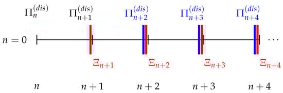
Figure 1.
Time-line of the discrete time dynamical system. The simulation starts by assuming a distribution tariff . Then, at every time step, there is a transition consumer → prosumer leading to a change in the aggregated apparent consumption . This change induces an adjustment of the distribution tariff .
The first billing period is necessary so that the consumers can observe their electricity bill under the initial conditions. Then, the transition consumer → prosumer can be computed, and, from it, we determine the total apparent consumption (which corresponds to the period to ). Since the consumption during the period n to and the consumption under the initial conditions are the same, the distribution tariff does not change (). However, once is computed, it induces a change in the distribution tariff for the following period (after the DSO observation of its revenue during the period to ). We assume that the consumers can react immediately to this distribution tariff adjustment since they already have knowledge regarding their consumption. Then, the aggregated apparent consumption can be calculated. The discrete time dynamical system continues in this fashion until no more consumers can turn into prosumers, or until the stopping criteria are met: when reaching the finite time horizon N, or when the DER are not economically profitable.
Every time step of the discrete time dynamical system, except for the first one, is computed with one run of our simulator. Thus, the developed simulator is run recursively to simulate the complete dynamical system. The end of one run will be used as starting point for the next one. The flow diagram representing an outline of one run of the simulator can be found in Figure 2.
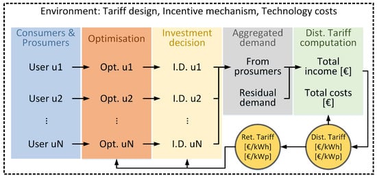
Figure 2.
Flow diagram of the proposed multi-agent simulator. The flow of actions occurs from left to right. The distribution network consumers undergo individual MILP optimisations to minimise their LCOEs. A transition consumer → prosumer is computed (investment decision tab (yellow) on the Figure), and finally the DSO adjusts the distribution tariff.
The simulation starts with a pool of consumers who may become prosumers at any point of our discrete time dynamical system. These agents, characterised by their load, are modelled through an MILP to plan and operate a DER installation minimising their LCOEs. Such an optimisation requires the retail electricity price at each time step, as well as the demand profile of the consumers. After the optimisation, a transition consumer → prosumer is computed by comparing the costs of the consumers with and without DER installation. The aggregated apparent consumption is then calculated and added to the residual demand of the system (those consumers of the distribution network who cannot deploy DER due to technical or economic constraints). Finally, the DSO revenues are computed, and, assuming constant costs across the discrete time dynamical system, the distribution tariff for the following time step is determined so as to fully recover those costs.
4. Modelling the Regulatory Framework
In this simulator, we introduce the concept of environment as the container of the set of rules that characterise the distribution network, namely the tariff design, the incentive mechanism, and the technology costs. Hence, to model the agents actions, we must take into account the distinct possible environments. Every single agent takes individual actions; therefore, we need to introduce the set representing the consumers/prosumers, where I is the number of consumers/prosumers. In the following, we present the differences in the simulator, depending on the tariff design and the incentive mechanism.
4.1. Tariff Design
We may use a fully volumetric design, or a two-part design with a variable (volumetric) and a fixed (per connection) term.
4.1.1. Fully Volumetric
Under this setting, the individual electricity costs of the agents in I are calculated as follows:
where represents the individual apparent consumption of the ith prosumer at the nth time step, is the distribution tariff set by the DSO, and represents the costs of energy, transmission and taxes, held constant across the simulation.
The DSO revenues are calculated as:
with being the residual demand of the system (held constant), and is the aggregated apparent consumption of the consumers/prosumers, which is calculated as
4.1.2. Two Part
In this case, we introduce a fixed term in the calculations. The electricity costs of the consumers/prosumers are calculated as follows:
where the term is set at the beginning of the simulation (see Equation (8)) and kept constant. As for the DSO, its revenues are computed as follows:
where , with J being the amount of consumers who make up the residual demand .
4.2. Incentive Mechanism
We may use NM and NB. This choice impacts the individual apparent consumption, and, as such, the aggregated one.
4.2.1. NM
The individual apparent consumption of the consumers/prosumers is given by:
where and are, respectively, the imports and exports of the ith prosumer at the nth time step.
4.2.2. NB
In this case, the exports do not affect the apparent consumption, thus:
4.3. Distribution Tariff Update
For every option of tariff design and incentive mechanism, the distribution tariff is updated at every time-step according to the following equation:
where are the costs of the DSO, which are calculated as the revenues of the first time step , and held constant across the dynamical system. The imbalance from the previous period is introduced with the difference . In other words, represents the costs of the DSO, represents the “missing money” from previous periods, and C represents the money recovered through fix charges, and the sum of these parameters thus represents a quantity in €. Then, represents the residual demand of the system (only consumers), represents the demand of the prosumers, and the sum of these parameters is therefore a quantity in kWh. The mechanism works in a way the tariff is updated according to costs divided by demand.
5. Case Study
To assess the impact of different environments on the distribution network evolution, we introduce a case study in which we compare nine different environments (regulatory frameworks). The simulator necessitates a set of consumers/prosumers to work. Each consumer/prosumer is characterised by a demand profile and a production profile. Once we have produced the set of consumers/prosumers, we evaluate: (i) four distinct designs with decreasing proportions of costs recovered through volumetric charges being replaced by fixed ones (where the incentive mechanism is kept fixed for all of them), and (ii) five different incentive mechanisms (where the proportion of volumetric charges is kept fixed for all of them). The different assessed environments are presented next.
- Different proportions of volumetric and fixed charges:
- -
- E1: environment with 100% volumetric charges. NB is used as incentive mechanism with a selling price of 4c€.
- -
- E2: environment with 75% volumetric charges and 25% fixed charges. NB is used as incentive mechanism with a selling price of 4c€.
- -
- E3: environment with 50% volumetric charges and 50% fixed charges. NB is used as incentive mechanism with a selling price of 4c€.
- -
- E4: environment with 25% volumetric charges and 75% fixed charges. NB is used as incentive mechanism with a selling price of 4c€.
- Different incentive mechanisms:
- -
- E5: environment with 100% volumetric charges. NM is used as an incentive mechanism.
- -
- E6: environment with 100% volumetric charges. NB is used as incentive mechanism with a selling price of 4c€. Note that this is the same as E1, but for the sake of clarity is used with the two names.
- -
- E7: environment with 100% volumetric charges. NB is used as an incentive mechanism with a selling price of 6c€.
- -
- E8: environment with 100% volumetric charges. NB is used as an incentive mechanism with a selling price of 8c€.
- -
- E9: environment with 100% volumetric charges. NB is used as an incentive mechanism with a selling price of 10c€.
For all of the environments, we set the value of to 0.132 €/kWh. Furthermore, we assume an initial distribution tariff of 0.088 €/kWh (making an equivalent retail price of 0.22 €/kWh). To determine two-part tariffs (E2 - E4), we compute:
where is the percentage of volumetric charges, and is an adjustment factor applied depending on the peak demand of the consumer/prosumer, which is useful to charge users fixed costs depending on their power consumption. In this case study, is assumed equal to 1 for all prosumers.
5.1. Results
To represent the distribution network evolution for each environment, we rely on four metrics: (i) the evolution of the variable (volumetric) term of the distribution tariff, (ii) the penetration of DER relative to the maximum potential I, (iii) the actual deployed PV and battery capacity (in kWp and kWh), and (iv) the LCOE of the deployed DER installations (in €/kWh).
5.1.1. Tariff Designs (E1–E4)
According to Figure 3, the upper-left subfigure, the variable (volumetric) term of the distribution tariff increases in a quicker fashion when the share of this term in the two-part tariff design is large. Likewise, the deployment of DER over time (Figure 3, lower-left subfigure) and the actual DER deployed capacity (Figure 4, upper subfigure), which represents the counterpart to the growth of the distribution tariff, increase in environments where the variable term in the two-part design is more prominent. In Figure 5, we can observe that the probability density functions of environments E1–E4 exhibit larger installation sizes for E1 (note that E1 and E6 represent the same environment) than E2, E3, and E4. Finally, regarding the LCOE of the DER installations, the four cases’ costs are similar to the equivalent retail price. Note that higher volume shares (E1) results in lower LCOEs. Finally, in Figure 6, the resulting LCOE of the prosumers is showcased. The red, dotted line indicates the electricity price (at the initialisation conditions) in €/kWh, without DER installation (i.e., for consumers).
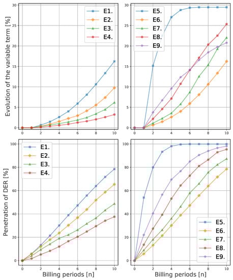
Figure 3.
Evolution of (upper two figures) and of the DER adoption (lower two figures) across the discrete time dynamical system, for the evaluation of tariff designs E1–E4 (left-hand side figures), and of the incentive mechanisms E5–E9 (right-hand side figures).
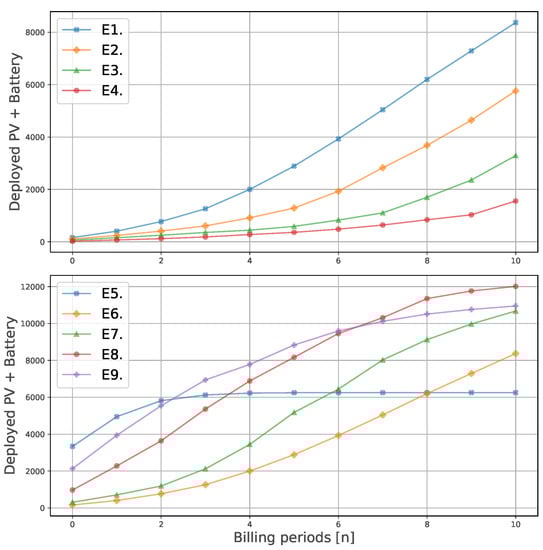
Figure 4.
Cumulative sum of the size of the deployed DER installations (including PV and batteries), over the discrete time dynamical system. The upper figure corresponds to the evaluation of tariff designs, whereas the lower one corresponds to the evaluation of the incentive mechanisms.
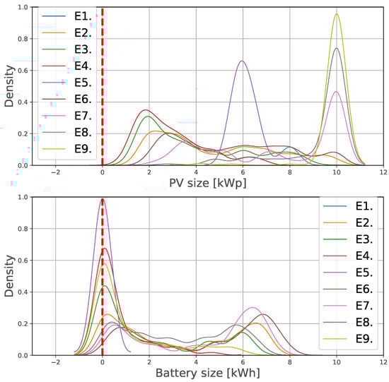
Figure 5.
Gaussian kernel density estimation of the installed capacity of PV (upper plot), and of batteries (lower plot). These figures represent the probability density function for the kernel density estimation of PV and battery capacities, for every environment (E1–E9). This probability is computed based on the calculated DER installation size of the set .
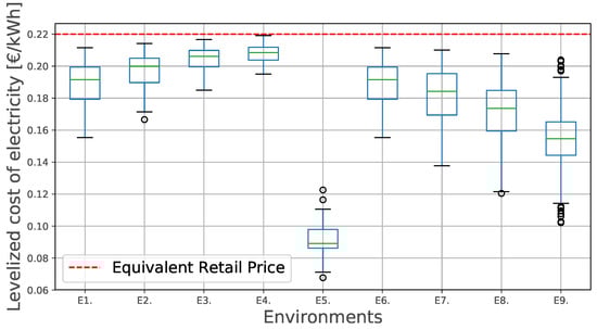
Figure 6.
Levelized cost of electricity of the prosumers in set , for every environment (E1–E9).
5.1.2. Incentive Mechanisms (E5–E9)
Figure 3, upper-right subfigure, shows two different trends, one for the NM environment (E5), and another for the rest. E5 variable term outgrows the other four by at least 5%, followed by E8, E7, E9, and E6 at the end (n = 10) of the simulation. The same trends are observed in Figure 3, lower-right subfigure, which represents the total DER penetration. However, examining the total capacities of deployed DER (Figure 4, lower subfigure, and Figure 5), it is visible that, despite the larger DER penetration, E5 results in lower total capacity of deployed PV and batteries. Regarding the LCOE, E5 displays a considerably lower LCOE than the rest of the environments. Figure 6 displays the resulting LCOE of the prosumers for scenarios E5 to E9, as well as for the previous ones (see Section 5.1.1 for more details).
5.2. Discussion
5.2.1. Tariff Designs (E1–E4)
We observe unity in the results, by increasing the share of the variable term in the distribution tariff, the business case to deploy DER installations improves, thus facilitating the transition consumer → prosumer. This, in turn, causes the distribution tariff to grow further in the environments with higher share of variable term, indicating a larger potential death spiral behaviour for those environments. Hence, introducing a two-part design reduces the instability of the system, as already highlighted in [31]. If we observe the total amount of PV and battery deployed (Figure 4), we can deduce that relying on distribution tariffs which are predominantly volumetric results in larger deployed DER capacities. This suggests a trade-off between DER penetration and total capacity installed, and a distribution price spiral. Such a trade-off must be addressed by policy makers in order to decide the desired trend. Finally, since the incentive mechanism in place (NB with a selling price of 0.04 €/kWh) does not significantly improve the DER business case, the four LCOEs are similar to the equivalent retail price, as can be seen in Figure 6. The lowest LCOE corresponds to E1, which is consistent with Figure 4 and Figure 5.
5.2.2. Incentive Mechanisms (E5–E9)
The different trends observed for NM and NB are a consequence of the distinct behaviour of prosumers they induce. With NM there is no incentive to make a business case selling electricity or becoming self-sufficient. NM offers the perfect scenario for the prosumers to adjust their production so that they import and export equivalent amounts of energy (). For this reason, the variable term in E5 (Figure 3), outgrows the other four environments, since the apparent consumption with E5 is close to zero, and the DSO needs to adjust the distribution tariff in a larger extent. We may also note that, under NM, no batteries are deployed (Figure 5). This is compatible with the findings in [5], where the authors observe that, with this system, batteries and imports are perfect substitutes. In Figure 6, we can the LCOE of these environments. The low LCOE of E5 is also consequence of the extremely low apparent consumption of the prosumers under NM. In the other four environments, the prosumers tend to deploy more PV and battery capacity to reduce their imports. Interestingly, when the selling price is high (E9), the prosumers rely on selling electricity as a business case, not reducing their apparent consumption in the same extent as E7 or E8. Hence, the increase in the distribution tariff is not so prominent in E9. A new trade-off appears between selling price and a distribution price spiral, where both imply an extra burden for the community.
6. Conclusions
In the context of increasing decentralised electricity generation, this paper has evaluated the effects of different regulatory frameworks on the evolution of distribution networks. A multi-agent model is used to simulate the behaviour of the agents of a distribution network. The actions of the agents are evaluated at several time-steps, leading to the evolution of the distribution network. Electricity consumers interacting with a single distribution network are modelled as rational agents that may invest in optimally sized distributed energy installations composed of PV and/or batteries. Finally, the distribution tariff is adapted according to the remuneration mechanism of the DSO.
We have designed and simulated four different examples based on gradually decreasing the proportion of volumetric charges switching them by fixed ones. Moreover, five different examples based on the type of incentive mechanism employed to promote DER are proposed. The results have been presented according to four distinct metrics: (i) the evolution of the volumetric term of the distribution tariff, (ii) the penetration of DER installations, (iii) the amount of deployed PV and batteries, and (iv) the LCOE of the deployed DER installations.
The results show that replacing volumetric charges with fixed ones impairs the economic business case of the consumers willing to deploy DER in the system. Regarding the use of different incentive mechanisms, using net-metering creates a potential spiral of the distribution tariff, with no integration of battery capacity in the system. When net-billing is used instead, the spiral of prices may be more easily contained by controlling the electricity selling prices. We observe a trade-off between spiralling electricity prices and the desired penetration of PV and batteries. Such trade-off may be tuned by policy makers by adjusting key parameters such as the level of capacity charges, or the selling price of electricity when net-billing is utilised.
This paper has analysed the different ways to foster DER adoption, and the regulatory challenges induced by them. Our approach is limited by the number of distribution network users who can be simulated, as well as by the assumption that only consumers whose electricity costs will decrease when deploying a DER installation may become prosumers. Future works could address a situation where the DSO allowed revenues do not remain constant throughout the simulation horizon; moreover, the use of non-rational agents may be addressed in the future.
Author Contributions
Conceptualization, D.E. and A.G.; methodology, M.M.d.V. and R.F.; software, M.M.d.V.; validation, M.M.d.V. and R.F.; investigation, M.M.d.V. and R.F.; resources, D.E.; data curation, M.M.d.V. and R.F.; writing—original draft preparation, M.M.d.V.; writing—review and editing, M.M.d.V., R.F., A.G. and D.E.; supervision, A.G. and D.E.; project administration, A.G.; funding acquisition, A.G. and D.E.
Funding
This research was funded by the public service of Wallonia within the framework of the TECR project.
Conflicts of Interest
The authors declare no conflict of interest. The funders had no role in the design of the study; in the collection, analyses, or interpretation of data; in the writing of the manuscript, or in the decision to publish the results.
Abbreviations
The following abbreviations are used in this manuscript:
| DER | Distributed energy resources |
| PV | Photovoltaic |
| FiT | Feed-in tariff |
| FiP | Feed-in premium |
| DSO | Distribution system operator |
| DG | Distributed generation |
| NM | Net-metering |
| NB | Net-billing |
| MILP | Mixed integer linear program |
| LCOE | Levelized cost of electricity |
| E# | Environment number |
References
- Study on the Effective Integration of Demand Energy Recourses for Providing Flexibility to the Electricity System; Final report to The European Commission; European Commission: Brussels, Belgium, 2015; p. 179.
- European Parliament, Council of the European Union. Directive 2009/28/EC of the European Parliament and of the Council of 23 April 2009 on the promotion of the use of energy from renewable sources and amending and subsequently repealing Directives 2001/77/EC and 2003/30/EC. Off. J. Eur. Union 2009, 5, 39–85. [Google Scholar]
- Candelise, C.; Winskel, M.; Gross, R.J. The dynamics of solar PV costs and prices as a challenge for technology forecasting. Renew. Sustain. Energy Rev. 2013, 26, 96–107. [Google Scholar] [CrossRef]
- Lopes, J.P.; Hatziargyriou, N.; Mutale, J.; Djapic, P.; Jenkins, N. Integrating distributed generation into electric power systems: A review of drivers, challenges and opportunities. Electr. Power Syst. Res. 2007, 77, 1189–1203. [Google Scholar] [CrossRef]
- Gautier, A.; Jacqmin, J.; Poudou, J.C. The prosumers and the grid. J. Regul. Econ. 2018, 53, 100–126. [Google Scholar] [CrossRef]
- Eid, C.; Guillén, J.R.; Marín, P.F.; Hakvoort, R. The economic effect of electricity net-metering with solar PV: Consequences for network cost recovery, cross subsidies and policy objectives. Energy Policy 2014, 75, 244–254. [Google Scholar] [CrossRef]
- Jargstorf, J.; Belmans, R. Multi-objective low voltage grid tariff setting. IET Gener. Transm. Distrib. 2015, 9, 2328–2336. [Google Scholar] [CrossRef]
- Costello, K.W.; Hemphill, R.C. Electric utilities’‘death spiral’: Hyperbole or reality? Electr. J. 2014, 27, 7–26. [Google Scholar] [CrossRef]
- Román, J.; Gómez, T.; Muñoz, A.; Peco, J. Regulation of distribution network business. IEEE Trans. Power Deliv. 1999, 14, 662–669. [Google Scholar] [CrossRef]
- Comnes, G.A. Review of Performance-Based Ratemaking Plans for US Gas Distribution Companies; Electricity Markets and Policy Group: Berkeley, CA, USA, 1994.
- Barker, P.P.; De Mello, R.W. Determining the impact of distributed generation on power systems. I. Radial distribution systems. In Proceedings of the Power Engineering Society Summer Meeting, Seattle, WA, USA, 16–20 July 2000; Volume 3, pp. 1645–1656. [Google Scholar]
- Ackermann, T.; Andersson, G.; Soder, L. Electricity market regulations and their impact on distributed generation. In Proceedings of the International Conference on Electric Utility Deregulation and Restructuring and Power Technologies. Proceedings (Cat. No.00EX382), London, UK, 4–7 April 2000; pp. 608–613. [Google Scholar]
- Pepermans, G.; Driesen, J.; Haeseldonckx, D.; Belmans, R.; D’haeseleer, W. Distributed generation: Definition, benefits and issues. Energy Policy 2005, 33, 787–798. [Google Scholar] [CrossRef]
- Reneses, J.; Ortega, M.P.R. Distribution pricing: Theoretical principles and practical approaches. IET Gener. Transm. Distrib. 2014, 8, 1645–1655. [Google Scholar] [CrossRef]
- Council of European Energy Regulators. Electricity Distribution Network TariffsCEER Guidelines of Good Practice; Technical Report; CEER: Brussels, Belgium, 2017. [Google Scholar]
- Ortega, M.P.R.; Pérez-Arriaga, J.I.; Abbad, J.R.; González, J.P. Distribution network tariffs: A closed question? Energy Policy 2008, 36, 1712–1725. [Google Scholar] [CrossRef]
- Pérez-Arriaga, I.J.; Jenkins, J.D.; Batlle, C. A regulatory framework for an evolving electricity sector: Highlights of the MIT utility of the future study. Econ. Energy Environ. Policy 2017, 6, 71–92. [Google Scholar]
- Cossent, R.; Gómez, T.; Frías, P. Towards a future with large penetration of distributed generation: Is the current regulation of electricity distribution ready? Regulatory recommendations under a European perspective. Energy Policy 2009, 37, 1145–1155. [Google Scholar] [CrossRef]
- European Commission. Study on Tariff Design for Distribution Systems; Technical Report; European Commission: Brussels, Belgium, 2015. [Google Scholar]
- De Joode, J.; Jansen, J.; Van der Welle, A.; Scheepers, M. Increasing penetration of renewable and distributed electricity generation and the need for different network regulation. Energy Policy 2009, 37, 2907–2915. [Google Scholar] [CrossRef]
- Frías, P.; Gómez, T.; Cossent, R.; Rivier, J. Improvements in current European network regulation to facilitate the integration of distributed generation. Int. J. Electr. Power Energy Syst. 2009, 31, 445–451. [Google Scholar] [CrossRef]
- Faerber, L.A.; Balta-Ozkan, N.; Connor, P.M. Innovative network pricing to support the transition to a smart grid in a low-carbon economy. Energy Policy 2018, 116, 210–219. [Google Scholar] [CrossRef]
- Picciariello, A.; Reneses, J.; Frias, P.; Söder, L. Distributed generation and distribution pricing: Why do we need new tariff design methodologies? Electr. Power Syst. Res. 2015, 119, 370–376. [Google Scholar] [CrossRef]
- Sotkiewicz, P.M.; Vignolo, J.M. Towards a cost causation-based tariff for distribution networks with DG. IEEE Trans. Power Syst. 2007, 22, 1051–1060. [Google Scholar] [CrossRef]
- González, A.; Gomez, T. Use of system tariffs for distributed generators. In Proceedings of the 16th Power Systems Computation Conference, Glasgow, UK, 14–18 July 2008. [Google Scholar]
- Christoforidis, G.; Panapakidis, I.; Papadopoulos, T.; Papagiannis, G.; Koumparou, I.; Hadjipanayi, M.; Georghiou, G. A model for the assessment of different net-metering policies. Energies 2016, 9, 262. [Google Scholar] [CrossRef]
- Laws, N.D.; Epps, B.P.; Peterson, S.O.; Laser, M.S.; Wanjiru, G.K. On the utility death spiral and the impact of utility rate structures on the adoption of residential solar photovoltaics and energy storage. Appl. Energy 2017, 185, 627–641. [Google Scholar] [CrossRef]
- Darghouth, N.R.; Barbose, G.; Wiser, R.H. Customer-economics of residential photovoltaic systems (Part 1): The impact of high renewable energy penetrations on electricity bill savings with net metering. Energy Policy 2014, 67, 290–300. [Google Scholar] [CrossRef]
- Darghouth, N.R.; Wiser, R.H.; Barbose, G.; Mills, A.D. Net metering and market feedback loops: Exploring the impact of retail rate design on distributed PV deployment. Appl. Energy 2016, 162, 713–722. [Google Scholar] [CrossRef]
- Gautier, A.; Jacqmin, J. PV adoption in Wallonia: The role of distribution tariffs under net metering. In Proceedings of the 7th Conference on the Regulation of Infrastructures, Bordeaux, France, 21–22 June 2018. [Google Scholar]
- Simshauser, P. Distribution network prices and solar PV: Resolving rate instability and wealth transfers through demand tariffs. Energy Econ. 2016, 54, 108–122. [Google Scholar] [CrossRef]
- Lesser, J.A.; Su, X. Design of an economically efficient feed-in tariff structure for renewable energy development. Energy Policy 2008, 36, 981–990. [Google Scholar] [CrossRef]
- Pyrgou, A.; Kylili, A.; Fokaides, P.A. The future of the Feed-in Tariff (FiT) scheme in Europe: The case of photovoltaics. Energy Policy 2016, 95, 94–102. [Google Scholar] [CrossRef]
- Sioshansi, R. Retail electricity tariff and mechanism design to incentivize distributed renewable generation. Energy Policy 2016, 95, 498–508. [Google Scholar] [CrossRef]
- Yamamoto, Y. Pricing electricity from residential photovoltaic systems: A comparison of feed-in tariffs, net metering, and net purchase and sale. Sol. Energy 2012, 86, 2678–2685. [Google Scholar] [CrossRef]
- Fridgen, G.; Kahlen, M.; Ketter, W.; Rieger, A.; Thimmel, M. One rate does not fit all: An empirical analysis of electricity tariffs for residential microgrids. Appl. Energy 2018, 210, 800–814. [Google Scholar] [CrossRef]
- Shang, Y. Hybrid consensus for averager–copier–voter networks with non-rational agents. Chaos Solitons Fractals 2018, 110, 244–251. [Google Scholar] [CrossRef]
- Abdelmotteleb, I.; Gómez, T.; Ávila, J.P.C.; Reneses, J. Designing efficient distribution network charges in the context of active customers. Appl. Energy 2018, 210, 815–826. [Google Scholar] [CrossRef]
- Manuel de Villena, M.; Gautier, A.; Fonteneau, R.; Ernst, D. A multi-agent approach to model the interaction between distributed generation deployment and the grid. In Proceedings of the CIRED Workshop 2018, Ljubljana, Slovenia, 7–8 June 2018. [Google Scholar]
- Prata, R.; Carvalho, P.M. Self-supply and regulated tariffs: Dynamic equilibria between photovoltaic market evolution and rate structures to ensure network sustainability. Util. Policy 2018, 50, 111–123. [Google Scholar] [CrossRef]
- Schittekatte, T.; Momber, I.; Meeus, L. Future-proof tariff design: Recovering sunk grid costs in a world where consumers are pushing back. Energy Econ. 2018, 70, 484–498. [Google Scholar] [CrossRef]
- Manuel de Villena, M.; Fonteneau, R.; Gautier, A.; Ernst, D. Exploring Regulation Policies in Distribution Networks through a Multi-Agent Simulator. In Proceedings of the YRS2018, Brussels, Belgium, 24–25 May 2018. [Google Scholar]


© 2019 by the authors. Licensee MDPI, Basel, Switzerland. This article is an open access article distributed under the terms and conditions of the Creative Commons Attribution (CC BY) license (http://creativecommons.org/licenses/by/4.0/).