Influence Analysis and Optimization of Sampling Frequency on the Accuracy of Model and State-of-Charge Estimation for LiNCM Battery

Abstract

Battery characterization data is the basis for battery modeling and state estimation. It is generally believed that the higher the sampling frequency, the finer the data, and the higher the model and state estimation accuracy. However, scientific selection strategy for sampling frequency is very important but rarely studied. This paper studies the influence of sampling frequency on the accuracy of battery model and state estimation under four different sampling frequencies: 0.2 Hz, 1 Hz, 2 Hz, and 10 Hz. Then, a function is proposed to depict the relationship between accuracy and sampling frequency, which shows an optimal selection principle. The iterative identification algorithm is presented to identify the model parameters, and state-of-charge (SOC) is estimated via extended Kalman filter algorithm. Experimental results with different operating conditions clearly show the relationship between sampling frequency, accuracy, and data quantity, and the proposed selection strategy has high practical value and universality.

1. Introduction

Due to the advantages of high specific energy, no memory effect, high cycle life, and low self-discharge rate, lithium-ion batteries are being largely adopted in electrical vehicles (EVs) [1]. To achieve safe and efficient operation of the power batteries under different driving conditions, it is urgent to use an advanced battery management system (BMS). It is one of the vital tasks of the BMS to monitor the state of the power battery, such as state-of-charge (SOC), state-of-power (SOP), and state-of-health (SOH) [2,3,4]. Since these parameters are not directly measured by existing on-board sensors, they need to be estimated, generally from model-based estimation algorithms. Therefore, the accuracy of the model is critical.

Several different kinds of battery models have been proposed in literature, which can be generally classified into white-box models, gray-box models, and black-box models [5]. White-box battery models are based on complex mathematical equations to describe the distributed electrochemistry reactions in the electrodes and electrolyte [6]. Although the white-box model has high precision, it is composed of multiple complex partial differential equations with a great many unknown parameters. Thus, the calculation process is complex. Compared with this type of battery models, the gray-box battery models, namely, equivalent circuit models (ECMs), are widespread used because such models not only can well obtain the dynamical behaviors of the battery but also have simple structure for computation and analysis. They have a high potential with respect to accuracy and parameterization effort [7]. The representative ECMs are the resistance (Rint) model, the Partnership for a New Generation of Vehicle (PNGV) model, and the resistance–capacitance (RC) model [8,9,10,11]. In comparison with the above-mentioned battery models, black-box battery models relate to models which are based on machine learning techniques, like neuronal network, fuzzy logic, or evolutionary algorithms, etc. [5]. In these models, the battery is treated as a black-box and the internal electrochemical process is ignored, which makes such battery models simple in structure and fast in simulation. However, different from the above two types of battery models, the main disadvantages of the black-box battery model are low estimation accuracy and high parameterization effort [5]. In summary, each battery model has its advantages and disadvantages. It is necessary to make a choice between the complexity and accuracy of the battery model according to the actual situation.

A major work in battery modeling is to identify the model parameters using some experimental data. In Reference [12], the analytical time domain-based method is selected to identify the model parameters with the voltage data of rest period. To improve the model accuracy, the voltage data of both the discharging and rest periods are used to identify the parameters based on the nonlinear least square algorithm in Reference [1]. However, batteries are alternately in charging, discharging, and relaxation modes during the operation of EV. Our ideas have been verified in Reference [13], in which we developed an iterative parameter identification method that can identify parameters under different conditions and make the battery model more accurate.

The SOC is a significant indicator of the battery, which directly shows the amount of residual energy. Estimating the SOC accurately can protect the battery from overcharged or overdischarged situations to avoid runaway, which can improve the battery performance and prolong the battery life [11]. A variety of methods have been developed to estimate the SOC, including ampere-hour (Ah) counting [14], open-circuit voltage (OCV) [15], artificial neural networks (ANN) [16], Kalman filter (KF) [17], etc. Each method has its advantages as well as disadvantages [1,18].

It is worth noting that the experimental data used to identify the parameters is closely related to the sampling frequency. The higher the sampling frequency, the more accurately the collected data can reflect the charging and discharging characteristics of the battery. Therefore, the sampling frequency may have an impact on the accuracy of the model. The most commonly used sampling frequencies are 1 Hz and 10 Hz [11,15]. However, in the existing literature, the influence of different sampling frequencies on the accuracy of the battery model has hardly been reported.

Aiming to study the influence of sampling frequency on the accuracy of the model and SOC estimation, firstly, a polynomial function is proposed to depict the relationship between accuracy and sampling frequency. Secondly, the second-order RC ECM is applied to describe the dynamic behavior of a lithium-ion battery, and the iterative identification algorithm is utilized to identify the model parameters. Furthermore, SOC is estimated by the extended Kalman filter (EKF) algorithm. Finally, several tests are designed to verify the accuracy of the battery model and SOC estimation at different sampling frequencies, and the strategy for reasonably selecting the sampling frequency is given.

2. Battery Model and SOC Estimation

2.1. Battery Model

A suitable battery model is required to guarantee the accuracy of state estimation. As mentioned in Section 1, a widely used approach for simulating batteries is the gray-box battery model because such models have a simple structure and can accurately reproduce battery dynamics over a wide frequency range. The popular ECM for batteries is the RC model, which is composed of resistor and parallel RC network(s) connected in series, such as the first-order RC [19,20], the second-order RC [21,22], and the third-order RC models [23]. Although adding more RC networks is helpful for enhancing the model accuracy, it brings as a result to the computation burden [2]. Consequently, it is vital to keep a balance between model accuracy and complexity.

In this paper, the second-order RC ECM is selected to simulate the dynamic behavior of lithium-ion battery. Figure 1 illustrates the schematic diagram of the utilized model, where U_oc represents the open-circuit voltage related to SOC; R₀ is the measured resistance; R₁ and C₁ indicate the electrochemical polarization resistance and capacitance, respectively; R₂ and C₂ denote the concentration polarization resistance and capacitance, respectively; i represents the working current which is positive during the discharge process and negative during the charge process; and U is the terminal voltage.

Under a current i (positive for discharge), the terminal voltage U is modeled as

$$\{\begin{array}{l}U=U_{oc}-i{R}_0-U_1-U_2\\ \frac{d{U}_1}{dt}=\frac{i}{C_1}-\frac{U_1}{C_1{R}_1}\\ \frac{d{U}_2}{dt}=\frac{i}{C_2}-\frac{U_2}{C_2{R}_2}\end{array}$$

(1)

where U₁ and U₂ indicate the voltage of capacitance C₁ and C₂, respectively. Uoc is the open-circuit voltage (OCV), which is usually a nonlinear function of SOC.

As mentioned in the notes of Equation (1), OCV is a function of SOC. There are different candidate models to fit the relationship between OCV and SOC [24,25,26]. In Reference [26], a sixth-degree polynomial function was reported to describe the OCV–SOC relationship most precisely:

$$y={\alpha }_0+{\alpha }_1{x}^6+{\alpha }_2{x}^5+{\alpha }_3{x}^4+{\alpha }_4{x}^3+{\alpha }_5{x}^2+{\alpha }_{6}x$$

(2)

where ${\alpha }_i$ (i = 0, 1, …, 6) is the pending coefficient, y represents the OCV, and $x$ represents the SOC.

The Ah counting shown by Equation (3) is a commonly used approach of estimating battery SOC, and is an easy and reliable implementation [27].

$$\mathrm{SOC}={\mathrm{SOC}}_0-\frac{1}{C_N}{\displaystyle \underset{0}{\overset{t}{\int }}\eta I}d\tau$$

(3)

where ${\mathrm{SOC}}_0$ is the initial SOC, $\eta$ is the charging–discharging efficiency, $I$ is the battery current, and $C_N$ is the usable charge capacity of the battery, which is recommended to measure firstly.

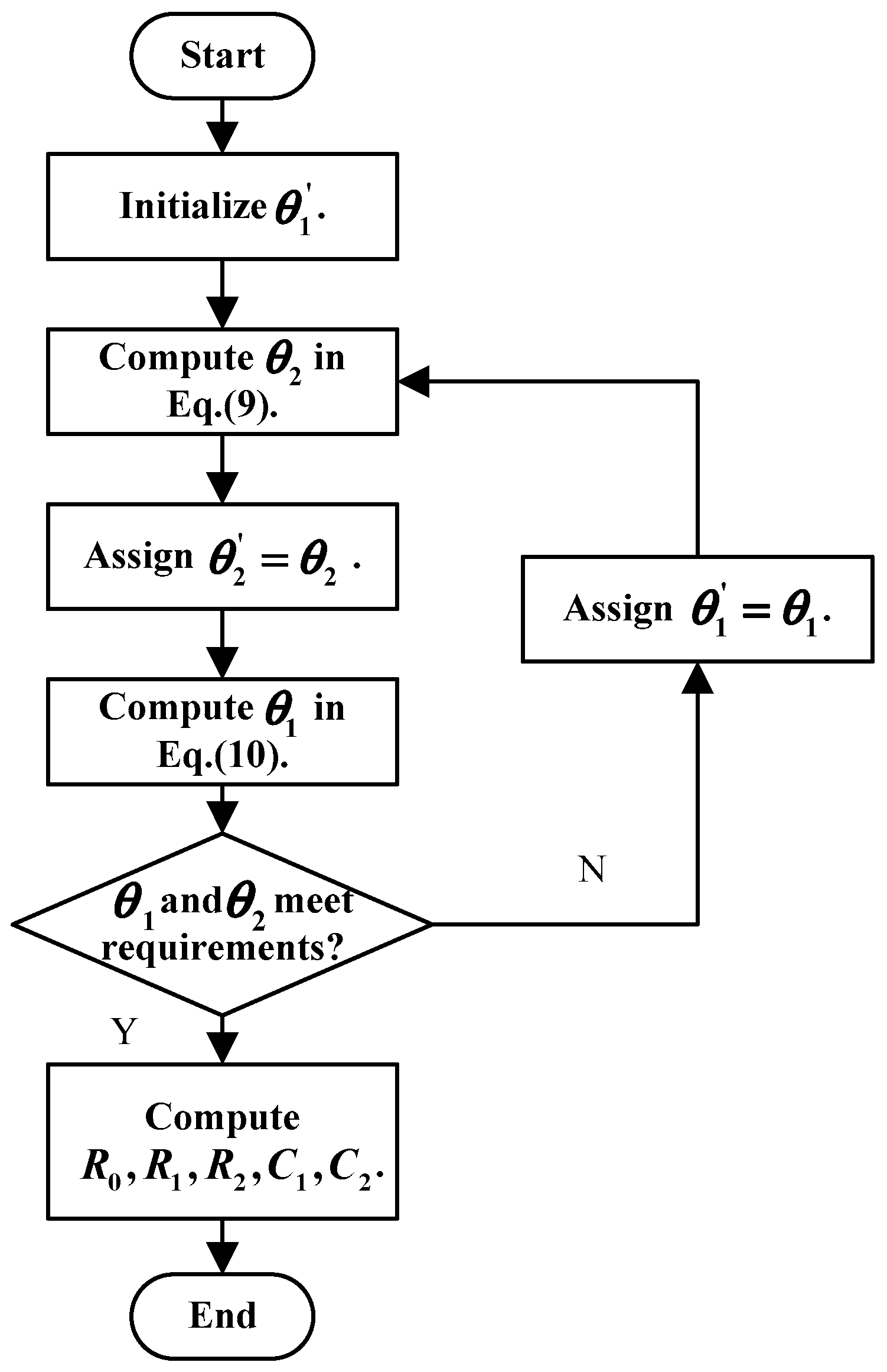
2.2. Parameters Identification Based on Iterative Identification Algorithm

The transfer function of the second-order RC ECM can be expressed as

$$G(s)=\frac{U_{ocv}(s)-U(s)}{I(s)}=\frac{V(s)}{I(s)}=R_0+\frac{R_1}{1+R_1{C}_{1}s}+\frac{R_2}{1+R_2{C}_{2}s}=\frac{b_0{s}^2+b_{1}s+b_2}{s^2+a_{1}s+a_2}$$

(4)

where $b_0=R_0$, $b_1=\frac{R_0{C}_1{R}_1+R_0{C}_2{R}_2+R_1{C}_2{R}_2+R_2{C}_1{R}_1}{C_1{R}_1{C}_2{R}_2}$, $b_2=\frac{R_0+R_1+R_2}{R_0{C}_1{R}_1{C}_2{R}_2}$, $a_1=\frac{C_1{R}_1+C_2{R}_2}{C_1{R}_1{C}_2{R}_2}$, $a_2=\frac{1}{C_1{R}_1{C}_2{R}_2}$.

The zero-order holder is used to obtain the discrete-time battery model. Hence Equation (4) yields to

$$\begin{array}{l}G(z)=\mathbb{Z}(G_h(s)G(s))\\ =\mathbb{Z}(\frac{1-e^{-Ts}}{s}\frac{b_0{s}^2+b_{1}s+b_2}{s^2+a_{1}s+a_2})\stackrel{z=e^{Ts}}{\to }(1-z^{-1})\mathbb{Z}(\frac{1}{s}\frac{b_0{s}^2+b_{1}s+b_2}{s^2+a_{1}s+a_2})\end{array}$$

(5)

where $\mathbb{Z}(·)$ is the notation of the z-transform.

After calculation, Equation (5) can be simplified as

$$G(z)=\frac{V(z)}{I(z)}=\frac{b_0^{\prime }{z}^2+b_1^{\prime }z+b_2^{\prime }}{z^2+a_1^{\prime }z+a_2^{\prime }}=\frac{b_0^{\prime }+b_1^{\prime }{z}^{-1}+b_2^{\prime }{z}^{-2}}{1+a_1^{\prime }{z}^{-1}+a_2^{\prime }{z}^{-2}}$$

(6)

where the coefficients are connected with the circuit parameters in Figure 1 and the sampling time T.

Consequently, we can compute R₀, R₁, C₁, R₂, and C₂ from Equation (6). In order to obtain the value of $a_1^{\prime }$, $a_2^{\prime }$, $b_0^{\prime }$, $b_1^{\prime }$, and $b_2^{\prime }$, it is necessary to $\mathbb{Z}$ inversely transform Equation (6):

$$V(k)=-a_1^{\prime }V(k-1)-a_2^{\prime }V(k-2)+b_0^{\prime }I(k)+b_1^{\prime }I(k-1)+b_2^{\prime }I(k-2)$$

(7)

Then, Equation (7) is written as

$$\{\begin{array}{l}{a}_1^{\prime }V(k-1)+a_2^{\prime }V(k-2)+V(k)=[\begin{array}{ccc}I(k)& I(k-1)& I(k-2)\end{array}]{[\begin{array}{ccc}{b}_0^{\prime }& b_1^{\prime }& b_2^{\prime }\end{array}]}^T\\ b_0^{\prime }I(k)+b_1^{\prime }I(k-1)+b_2^{\prime }I(k-2)-V(k)=[\begin{array}{cc}V(k-1)& V(k-2)\end{array}]{[\begin{array}{cc}{a}_1^{\prime }& a_2^{\prime }\end{array}]}^T\end{array}$$

(8)

Denote ${\theta }_1={\left[a_1^{\prime },a_2^{\prime }\right]}^T$, ${\theta }_2={\left[b_0^{\prime },b_1^{\prime },b_2^{\prime }\right]}^T$. Figure 2 illustrates the flowchart of parameter iterative identification and the specific steps of this method are as follows.

Step 1: Set the initial value of the parameter ${\theta }_1$ according to the system characteristics and assume ${\theta }_1^{\prime }={\left[a_1^{\prime },a_2^{\prime }\right]}^T$.

Step 2: Identify ${\theta }_2$ by the least square (LS) method, the formula can be written as

$${\theta }_2=(I^{T}I{)}^{-1}{I}^{T}V$$

(9)

where $I=\left[I(\mathrm{k}),I(k-1),I(k-2)\right]$ and $V=V(k)+\left[V(k-1),V(k-2)\right]{\theta }_1^{\prime }$. It is worth noting that $b_0^{\prime }>0$, $b_1^{\prime }<0$, $b_2^{\prime }>0$. If a certain parameter $b_{\mathrm{i}}^{\prime }$ in the vector ${\theta }_2$ does not meet the requirements, assign $b_{\mathrm{i}}^{\prime }=0$;

Step 3: Take the above parameters ${\theta }_2$ into the second one of (8), i.e., ${\theta }_2^{\prime }={\theta }_2$ and utilize the LS to identify ${\theta }_1$ again:

$${\theta }_1=(V^{\prime T}{V}^{\prime }{)}^{-1}{V}^{\prime T}{I}^{\prime }$$

(10)

where $I^{\prime }=-V(k)+\left[I(k),I(k-1),I(k-2)\right]{\theta }_2^{\prime }$ and $V^{\prime }=\left[V(k-1),V(k-2)\right]$. It is worth noting that $a_1^{\prime }<0$, $a_2^{\prime }>0$. If a certain parameter $a_{\mathrm{i}}^{\prime }$ in the vector ${\theta }_1$ does not meet the requirements, assign $a_{\mathrm{i}}^{\prime }=0$.

Step 4: If both ${\theta }_1$ and ${\theta }_2$ meet the system requirements shown in Equation (11), stop the iterations. Otherwise, go back to Step 2.

$$\Delta =\left|X_{\mathrm{m}}-X_t\right|\le \epsilon$$

(11)

where X_m is the model output and X_t is the true value. $\epsilon$ is set according to the actual situation.

Step 5: According to ${\theta }_1$, ${\theta }_2$, and Equation (6), the parameters R₀, R₁, C₁, R₂, and C₂ can be obtained.

The parameters of the second-order RC ECM can be identified by utilizing the above method. Besides, the data collected from charging, discharging, and rest periods can be used to identify the model parameters under different SOC.

2.3. SOC Estimation

The discretization calculation of Equation (1) can be expressed as

$$\{\begin{array}{l}{U}_{t,k}=U_{oc,k}-U_{1,k}-U_{2,k}-i_k{R}_0\\ U_{1,k+1}=U_{1,k}{e}^{-T/{\tau }_1}+i_k{R}_1\left(1-e^{-T/{\tau }_1}\right)\\ U_{2,k+1}=U_{2,k}{e}^{-T/{\tau }_2}+i_k{R}_2\left(1-e^{-T/{\tau }_2}\right)\end{array}$$

(12)

where U_t,k, U_oc,k, U_j,k (j = 1, 2), and i_k are the terminal voltage, the OCV, the polarization voltage, and the load current at the kth sampling time, respectively; T is the sampling time and ${\tau }_j=R_j{C}_j$ (j = 1, 2) is the time constant.

The discrete-time form of (3) can be written as

$${\mathrm{SOC}}_{k+1}={\mathrm{SOC}}_k-i_k\left(\eta T/C_N\right)$$

(13)

where SOC_k and i_k are the SOC and the current at the kth sampling time, respectively.

Based on Equations (12) and (13), the state space equation of the battery system can be obtained as

$$\{\begin{array}{l}\left[\begin{array}{l}{\mathrm{SOC}}_{k+1}\\ U_{1,k+1}\\ U_{2,k+1}\end{array}\right]=\left[\begin{array}{ccc}1& 0& 0\\ 0& e^{\raisebox{1ex}{$-T$}\!\left/ \!\raisebox{-1ex}{${\tau }_1$}\right.}& 0\\ 0& 0& e^{\raisebox{1ex}{$-T$}\!\left/ \!\raisebox{-1ex}{${\tau }_2$}\right.}\end{array}\right]\left[\begin{array}{c}{\mathrm{SOC}}_k\\ U_{1,k}\\ U_{2,k}\end{array}\right]+\left[\begin{array}{c}\raisebox{1ex}{$\eta T$}\!\left/ \!\raisebox{-1ex}{$C_n$}\right.\\ R_1\left(1-e^{\raisebox{1ex}{$-T$}\!\left/ \!\raisebox{-1ex}{${\tau }_1$}\right.}\right)\\ R_2\left(1-e^{\raisebox{1ex}{$-T$}\!\left/ \!\raisebox{-1ex}{${\tau }_2$}\right.}\right)\end{array}\right]i_k\\ U_{t,k}=U_{oc,k}-U_{1,k}-U_{2,k}-i_k{R}_0\end{array}$$

(14)

Assuming i_k and U_t,k are input variables and output variables of the system, respectively, and the state vector is defined as $x_k={\left[\begin{array}{ccc}{\mathrm{SOC}}_k& U_{1,k}& U_{2,k}\end{array}\right]}^T$, the EKF algorithm is then introduced to estimate battery state, which constitutes a robust and efficient observer for nonlinear systems. The readers can consult References [18,28] for more details of the EKF algorithm. The specific steps of the EKF algorithm are described in

Table 1. Summary of the extended Kalman filter (EKF) algorithm for state-of-charge (SOC) estimation.

$\{\begin{array}{l}{x}_k=f\left(x_{k-1},u_{k-1}\right)+w_k,w_k\sim N\left(0,Q_k\right)\\ y_k=g\left(x_k,u_k\right)+v_k,v_k\sim N\left(0,R_k\right)\end{array}$

Definitions:$A_{k-1}=\frac{\partial f(x_{k-1}^{+},u_{k-1})}{\partial x_{k-1}}{|}_{x_{k-1}=x_{k-1}^{+}}$ and $C_k=\frac{\partial g(x_k^{-},u_k)}{\partial x_k}{|}_{x_k=x_k^{-}}$.

Initialization:

State variable: $x_0^{+}=E\left[x_0\right]$. Mean square estimation error: $P_0^{+}=E\left[\left(x_0-x_0^{+}\right){\left(x_0-x_0^{+}\right)}^T\right]$.

Time Update:

Prior estimate of state: $x_k^{-}=f\left(x_{k-1}^{+},u_{k-1}\right)$. Prior estimate of error covariance: $P_k^{-}=A_{k-1}{P}_{k-1}^{+}{A}_{k-1}^T+Q_{k-1}$.

Measurement Update:

Kalman gain matrix update: $K_k=P_k^{-}{C}_k^{-}{\left(C_k{P}_k^{-}{C}_k^T+R_k\right)}^{-1}$. Measurement update of state estimate: $x_k^{+}=x_k^{-}+K_k\left(y_k-g(x_k^{-},u_k)\right)$. Measurement update of error covariance: $P_k^{-}=\left(I-K_k{C}_k\right)P_k^{-}$.

.

3. Experiment

3.1. Battery Test Bench

As shown in Figure 3, the test bench consists of a NBT5V10AC16-T battery cycler for charging and discharging the battery, a programmable thermal chamber, a lithium-ion battery, and a host computer for programming and storing data. The battery cycler is produced by Ningbo Bayte Measurement and Control Technology Co., Ltd., which has sixteen dependent measurement channels with a voltage range of 0 to 5 V and current range of 0.3 to 10 A. The errors of the current and voltage sensors of the NBT5V10AC16-T battery cycler are both within 0.1%. All measured data of the battery voltage and current are transmitted to the host computer through TCP/IP port. The PC can program experiment procedure and deal with real-time data. The test object is Lishen’ s LR1865SZ lithium-ion battery, which has a nominal capacity of 2.5 Ah, nominal voltage of 3.6 V, charging cut-off voltage of 4.2 V, and discharging cut-off voltage of 3.0 V. The maximum charging and discharging current refer to the limit current when charging or discharging for a long time.

Table 2. Specifications for the test battery at 25 °C.

Parameter	LiNCM
Rated capacity	2500 mAh
Nominal voltage	3.6 V
Charging cut-off voltage	4.2 V
Discharging cut-off voltage	3.0 V
Maximum charging current	2.5 A (1C)
Maximum discharging current	7.5 A (3C)

shows the specific specification of the battery obtained from the manufacturer. To reduce the influence of temperature, the tested battery is kept in the thermal chamber with 25 °C.

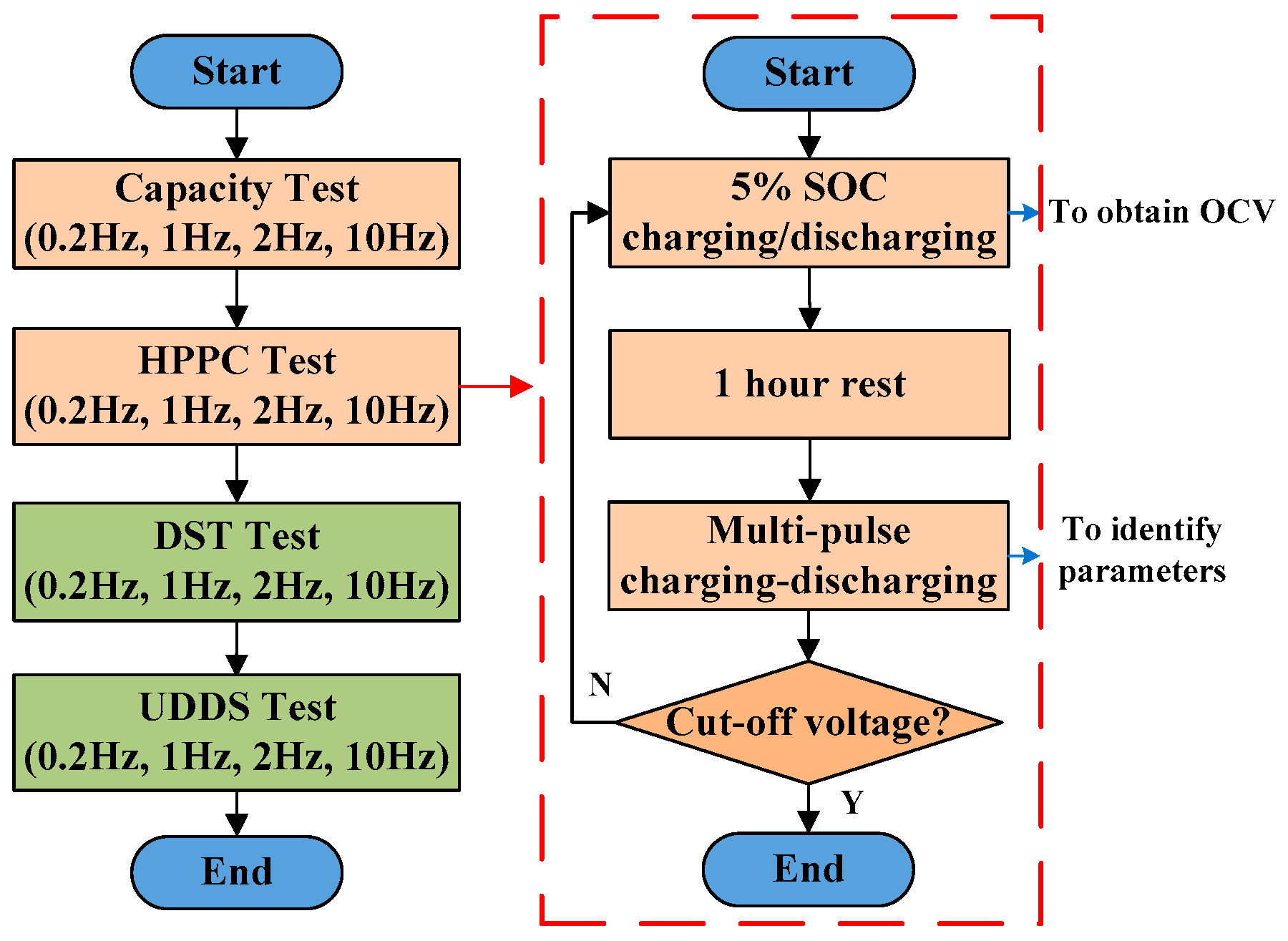
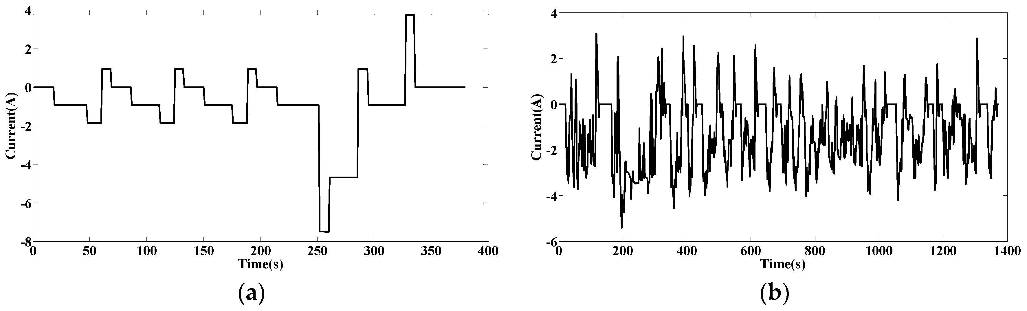
3.2. Battery Test Schedule

The test schedules shown in Figure 4 consist of a maximum capacity test, an improved Hybrid Pulse Power Characterization (HPPC) test, a Dynamic Stress Test (DST), and an Urban Dynamometer Driving Schedule (UDDS) test [2,13]. The purpose of the maximum capacity test is to measure the battery capacity. The improved HPPC is composed of a pulse discharging or charging profile and a multipulse charging–discharging profile. The discharging or charging pulse test, which aim to obtain a functional relationship between the SOC and OCV, is performed by discharging or charging at a constant current with an interval of 5% SOC, thereby circulating to the cutoff voltage. The multipulse charging–discharging test is conducted on the battery at 5% SOC intervals to identify the model parameters. At last, DST and UDDS are used to verify the accuracy of the model. In order to investigate the effect of sampling frequency on the accuracy of the model, the above tests need to be performed at four different sampling frequencies: 0.2 Hz, 1 Hz, 2 Hz, and 10 Hz. The specific steps of the above experiments are as follows.

First of all, the capacity test of the battery is conducted to obtain the maximum available capacity, which consists of constant current-constant voltage (CC-CV) charging and constant current (CC) discharging. The constant current is 1/3C. Here, 1C means the current is numerically equal to the nominal capacity.

Then, the charging OCV is measured based on the pulse charging test; the procedure is as follows. First, the battery is discharged fully and then rested for 1 h. Second, the battery is charged at charging rate of 1/3C from the fully discharged state to 5% of the nominal capacity. The terminal voltage is monitored after resting for 1 h, which is considered to be the charging OCV. The battery is continuously charged by a further 5% of the nominal capacity at the same current, and the charging OCV is measured after resting for 1h again. The pulse charging test is not finished until the terminal voltage reaches the upper cut-off voltage of the battery. Afterwards, pulse charging test data are used to fit the function to depict the charging OCV–SOC relationship according to Equation (2). The discharging pulse test is performed by discharging the battery at discharging rate of 1/3C from the fully charged state with a step of 5% of the nominal capacity. The pulse discharging test is not finished until the terminal voltage reaches the lower cut-off voltage of the battery. Similar to pulse charging test, the discharging OCV–SOC relationship can be obtained.

During the charging or discharging pulse test, a multipulse charging–discharging test is conducted on the battery at 5% SOC intervals in order to identify the model parameters, including R₀, R₁, R₂, C₁, and C₂. In this test, the battery is discharged and charged in 0.2C, 0.5C, and 1C. Specifically, the battery is discharged at constant current for 10 s, rested at zero current for 40 s, and subsequently charged at the same constant current for 10 s. The multipulse charging–discharging profile is shown in Figure 5.

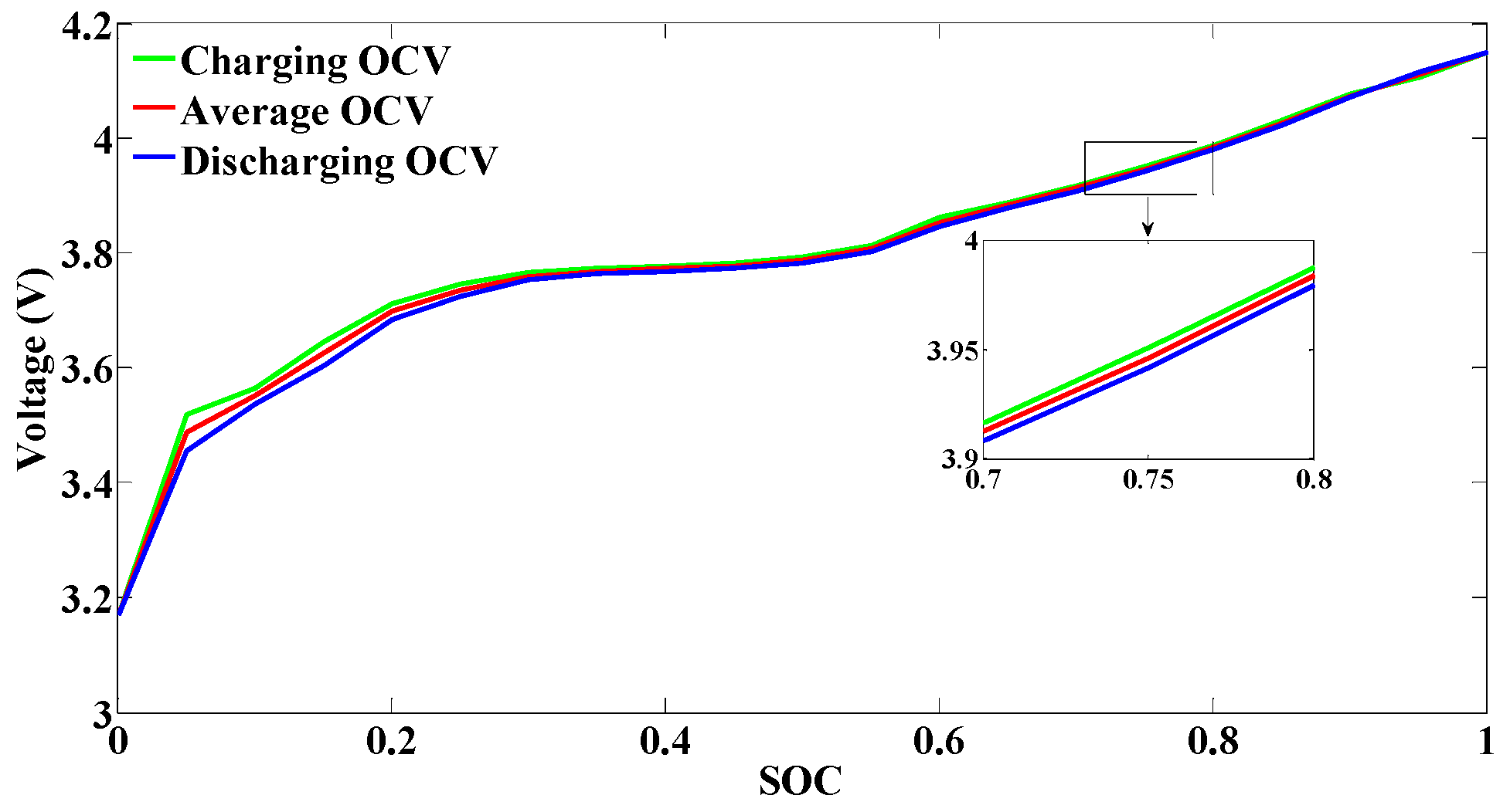
3.3. Experimental Results

To obtain real capacity of battery, the capacity test is repeatedly implemented three times under four different sampling frequencies, and the results are shown in

Table 3. Real capacity of battery at different sampling frequencies.

Sampling Frequency (Hz)	Measured Capacity (Ah)			Average Capacity (Ah)
0.2	2.502	2.504	2.503	2.503
1	2.500	2.501	2.505	2.502
2	2.507	2.502	2.503	2.504
10	2.503	2.506	2.501	2.503

. The average value of measured capacity is set as the capacity of the battery. It is obvious that the capacity is almost the same as the sampling frequencies of 0.2 Hz to 10 Hz, which means that the sampling frequency has little effect on the capacity.

Figure 6 illustrates the relationship between SOC and OCV for the battery at a sampling frequency of 1 Hz as an example. The green curve and the blue curve represent the charging OCV and discharging OCV, respectively. It can be found that a gap is observed between the charge and discharge OCV curves. The OCV is defined as the average of the two, shown as the red curve in Figure 6. In addition, the relationship between OCV and SOC is fitted by the polynomial function shown in Equation (2).

The parameters identified from the multipulse charging–discharging test under different SOCs and sampling frequencies are shown in Figure 7, and the average values of the parameters are listed in

Table 4. Average values of parameters at different sampling times.

Sampling Frequency (Hz)	Average R0 (ohm)	Average R1 (ohm)	Average R2 (ohm)	Average C1 (F)	Average C2 (F)
0.2	0.0416	0.0006	0.0350	2252.9	1523.9
1	0.0391	0.0025	0.0445	1095.4	1454.7
2	0.0367	0.0017	0.0419	772.1	1208.4
10	0.0290	0.0058	0.0464	1179.1	1389.4

. At different sampling frequencies, the resistances and the capacitances exhibit the same tendencies of SOC variation except some fluctuations. It is obvious from Figure 7a that R₀ exhibits prominent dependence on SOC and strong dependence on sampling frequency. R₀ decreases with the increase of SOC and reduces significantly with the increase of the sampling frequency. Based on Ohm’s law [12], the measured resistance R₀ is obtained from the ratio of the instantaneous voltage difference to the current at the same time, which consists of both ohmic resistance and a part of the polarization resistance [29]. The higher the sampling frequency, the smaller the influence of polarization resistance, and the smaller the identified R₀, as shown in Figure 7a. The sampling frequency also has an effect on other parameters. For R₁ and R₂, it can be seen that their values increase with the improvement of the sampling frequency, while the values of C₁ and C₂ are reduced. For the SOC dependence, R₁ and C₁ show minimal dependence on SOC; they seem to be fluctuating around a value. However, the relationship between R₂, C₂, and SOC is more complicated, as peaks and valleys are observed. R₂ drops to a nadir at 0.4 and reaches a peak at 0.6, whereas C₂ is the opposite (rises to a peak at 0.4 and declines to a nadir at 0.6).

4. Validation

In order to validate the model accuracy, DST and UDDS are adopted as inputs of the lithium-ion battery, whose current profile is shown in Figure 8. A DST cycle lasts for 380 s, including 20 transients. In this test, DST is carried out on a fully charged battery with −3.75 A as the maximum charging current and 7.5 A as the maximum discharging current. As shown in Figure 8b, the charging–discharging pulses of the UDDS test are more complicated. It is noteworthy that the model parameters at each SOC are obtained via an interpolation algorithm. The experimental voltage at different sampling frequencies need to be compared with the model predicted model voltage to study the effect of sampling frequency on model accuracy. In addition, EKF algorithm is utilized to estimate the SOC of the battery under DST test experiment, and the estimation results at different sampling frequencies are discussed.

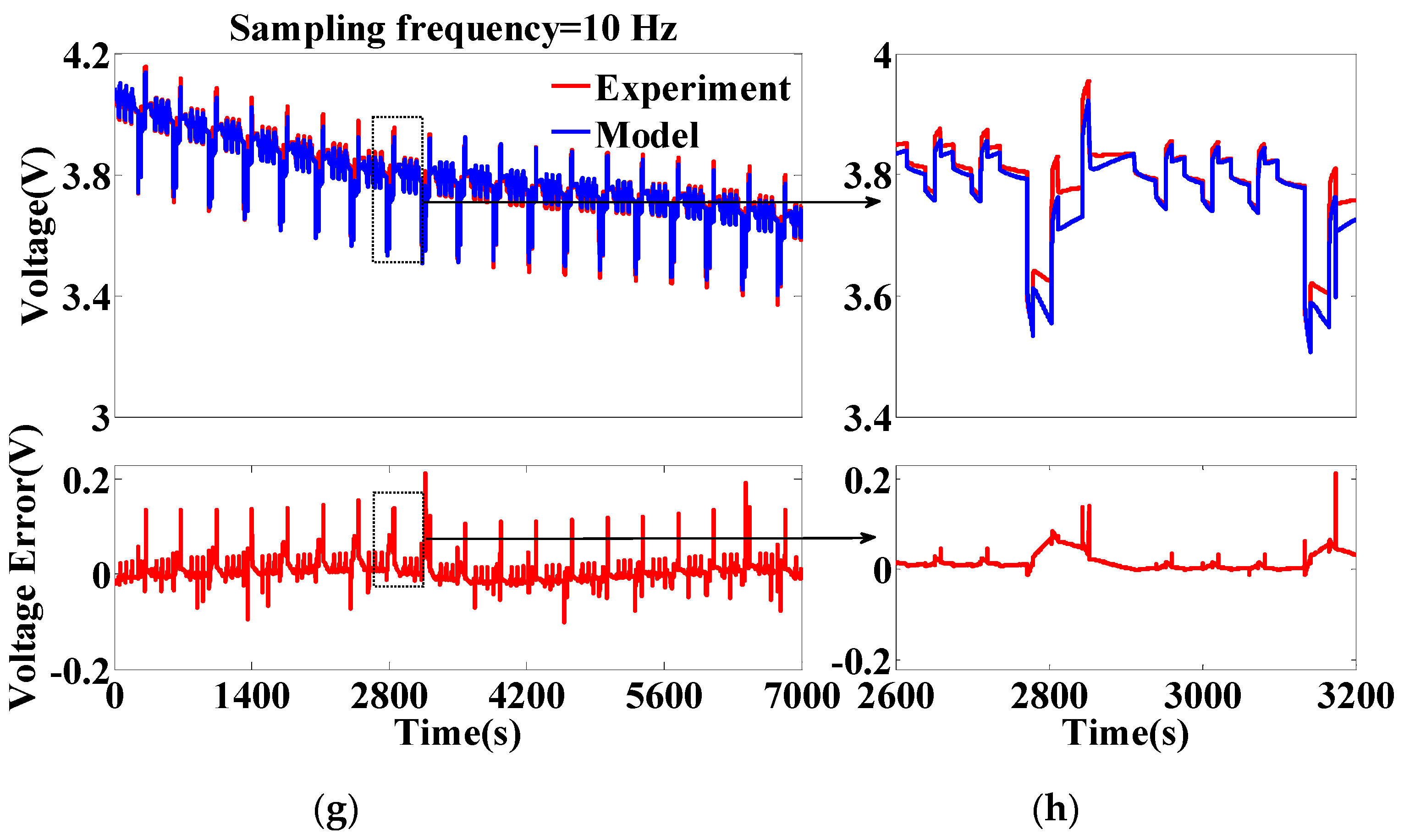
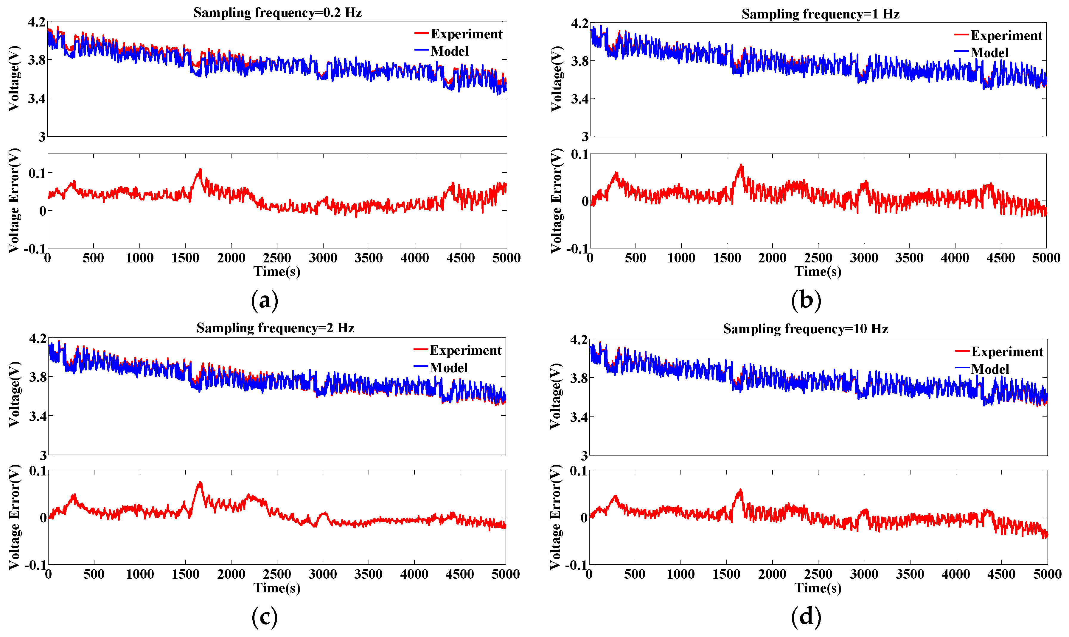
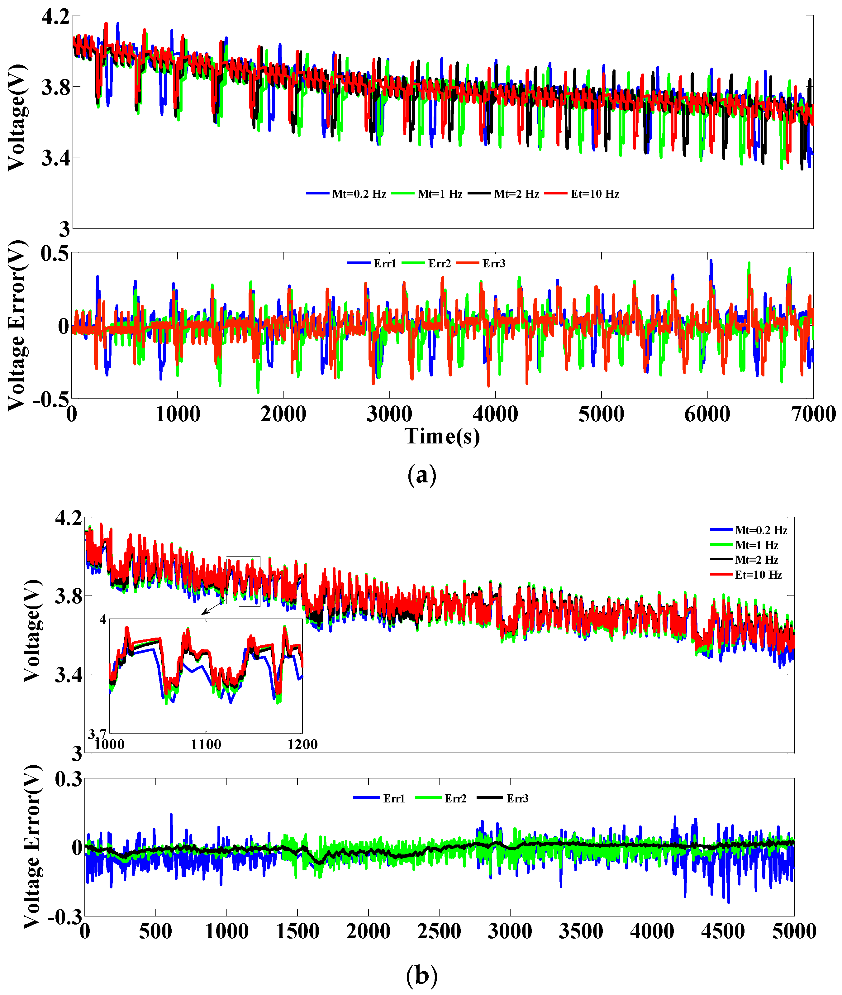
4.1. Voltage Response Results at Different Sampling Frequencies

The measured voltage and the model voltage at different sampling frequencies are plotted in Figure 9. The estimation results of terminal voltage under DST at sampling frequencies of 0.2 Hz, 1 Hz, 2 Hz, and 10 Hz are plotted in Figure 9a,c,e,g, respectively, while Figure 9b,d,f,h gives out the zoom figures, respectively.

The mean absolute error (MAE) and the root mean square error (RMSE) are adopted to further compare the accuracy to evaluate the estimation performance quantitatively. According to Figure 9, the MAEs under the DST test experiment at four different sampling frequencies were 33.4 mV, 16.5 mV, 13.5 mV, and 11.7 mV, respectively, while the RMSEs were 43 mV, 23.3 mV, 19.1 mV, and 16.6 mV, respectively. In addition, the maximum absolute estimation errors of estimated voltage at four different sampling frequencies were 324.4 mV, 322.8 mV, 239.9 mV, and 214.4 mV (7.72%, 7.69%, 5.71%, and 5.10% of its upper cut-off voltage), respectively.

As shown in Figure 9b,d,f,h, there are large errors at some points of the voltage curve, that is, the difference between the experimental value and the simulation value is large. Specifically, at low currents, the model voltage can follow the battery voltage very well. However, few large false values exist when the operating current is large (3C). It signifies that the identification method under large current conditions remains to be improved.

To illustrate universality, the estimation results of terminal voltage under UDDS test at four different sampling frequencies are plotted in Figure 10.

Table 5. Statistic list of voltage errors.

Sampling Frequency (Hz)	Working Condition	MAE (%)	RMSE (%)	Max Error (%)
0.2	DST	0.79	1.10	7.72
	UDDS	0.74	0.89	2.59
1	DST	0.39	0.55	7.69
	UDDS	0.53	0.47	1.82
2	DST	0.32	0.45	5.71
	UDDS	0.34	0.44	1.78
10	DST	0.28	0.39	5.10
	UDDS	0.29	0.37	1.40

gives the statistic result of the voltage errors, from which the specific error variations can be obtained. The percentage indicates the ratio of the error to the upper cut-off voltage. It shows that the MAE under DST test decreases obviously with the improvement of the sampling frequency, dropping from 33.4 mV at 0.2 Hz to 11.7 mV at 10 Hz, while the MAE under UDDS testing reduced from 31 mV to 12.3 mV. The higher sampling frequency causes the result with higher resolution, and it is helpful to differentiate the small changes of terminal voltage in a short time, which can improve the model accuracy.

In the above content, the difference between model voltage at a sampling frequency and the measured voltage at the same frequency is computed. The voltages Mt^0.2, Mt¹, and Mt² denote the model outputs at 0.2 Hz, 1 Hz, and 2 Hz, respectively. Voltage Et¹⁰ denotes the measurement voltage at 10 Hz. In order to clarify the variation of the model error with the sampling frequency, the model output voltages of Mt^0.2, Mt¹, and Mt² are compared, as well as the measurement voltage Et¹⁰, which is considered as the reference. The comparison results are shown in the Figure 11, where Err1 is the difference between Mt^0.2 and Et¹⁰. Err2 and Err3 are similar to Err1. It is obvious that the model output voltage is closer to the reference measurement voltage with the increase of the sampling frequency, especially in the zoom figure of (b).

Based on the above analysis, we can conclude that, on the one hand, the model and the parameter identification method are effective. On the other hand, the accuracy of model is improved with the improvement of the sampling frequency. However, the improvement of the sampling frequency increases the experimental data and affects the efficiency of the calculation. Therefore, it is important to strike a balance between the sampling frequency and the model accuracy.

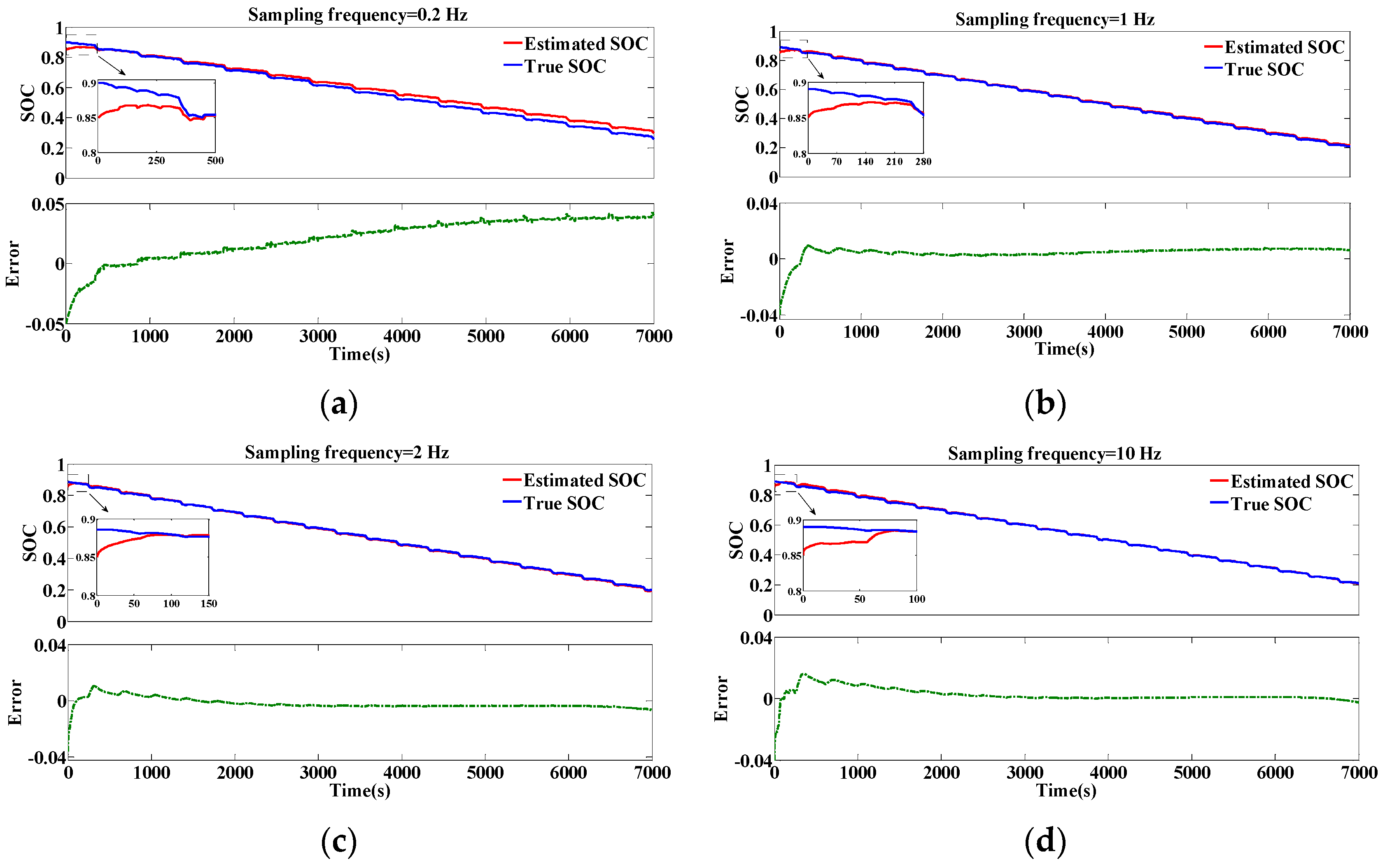
4.2. SOC Estimation Results at Different Sampling Frequencies

According to the EKF algorithm listed in Table 1, the SOC estimation results at different sampling frequencies are shown in Figure 12 and Figure 13, where the blue solid line and red solid line indicate the true and estimated SOCs, respectively, while the dashed line describes SOC error based on the model parameters obtained by the iterative identification algorithm. The true SOC is calculated using the Ah counting method. Shown in Figure 12a–d are the SOC estimation results under DST test experiments at sampling frequencies of 0.2 Hz, 1 Hz, 2 Hz, and 10 Hz, respectively, while Figure 13a–d shows the SOC estimation results of the UDDS tests.

In order to verify the robustness of the EKF algorithm, the initial SOC was set to 0.85. According to Figure 12, the MAEs of SOC estimation under DST at four different sampling frequencies are 2.4%, 0.6%, 0.4%, and 0.3%, respectively, while the RMSEs are 2.7%, 0.6%, 0.4%, and 0.5%, respectively. In addition, the maximum absolute errors of estimated SOC at four different sampling frequencies are 4.2%, 1.1%, 1.1%, and 1.6%, respectively. A similar comparison of the SOC estimation under UDDS testing is provided in Figure 13. The MAEs are 0.5%, 0.4%, 0.4%, and 0.3%, respectively, while the RMSEs are 1.1%, 1%, 0.7% and 0.8%, respectively. In addition, the maximum absolute errors are 1.5%, 1.3%, 1.1%, and 1.8% respectively.

The zoomed figures in Figure 12 and Figure 13 show that the big initial SOC error can be corrected quickly, which means that this algorithm is fast enough to correct the SOC error. The convergence time is defined as the time when the difference between the true SOC and the estimated SOC is less than 0.01 from the initial time. It can be seen that the convergence speed is gradually accelerated with the improvement of the sampling frequency. Furthermore, it can be seen that the estimated SOC in keeping with the measured one.

The maximum errors, MAEs, RMSEs, and convergence time of the SOC estimation at different sampling frequencies are summarized in

Table 6. Statistic list of SOC errors and convergence time.

Sampling Frequency (Hz)	Working Condition	MAE	RMSE	Max Error	Convergence Time (s)
0.2	DST	0.024	0.027	0.042	491
	UDDS	0.005	0.011	0.015	260
1	DST	0.006	0.006	0.011	269
	UDDS	0.004	0.01	0.013	247
2	DST	0.004	0.004	0.011	110
	UDDS	0.004	0.007	0.011	115
10	DST	0.003	0.005	0.016	86
	UDDS	0.003	0.008	0.018	110

. It shows that the MAEs of SOC estimation keep on decreasing with the improvement of the sampling frequency, which implies that the EKF estimation method is useful to improve SOC estimation accuracy through reducing the battery model error.

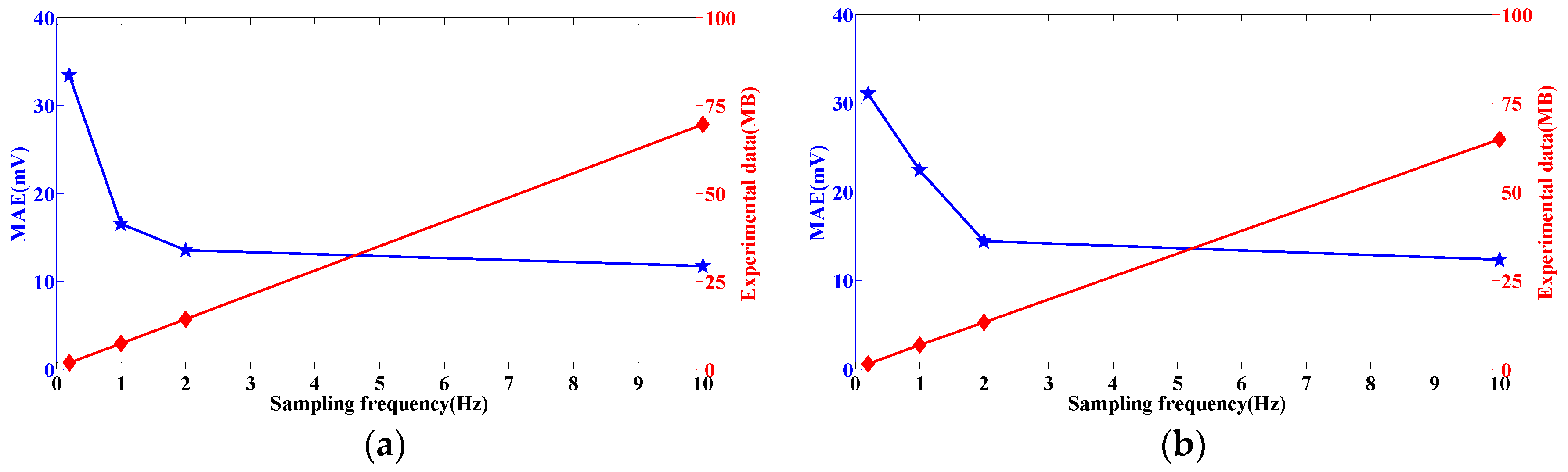
5. Quantitative Analysis and Optimal Selection

The error between the simulation and true values is typically used to reflect the accuracy of the battery model and SOC estimation. Theoretically, the higher the sampling frequency, the more data will be collected per second, which can reflect the changes of batteries in more detail and make the simulation more accurate. Therefore, the relationship between accuracy and sampling frequency can be expressed as

$$E_1\left(F\right)={\lambda }_{1}F+{\lambda }_2$$

(15)

where $E_1(·)$ is the error and ${\lambda }_1$ and ${\lambda }_2$ are the pending coefficients.

However, it is possible to acquire a large number of interfering signals with the improvement of sampling frequency, which causes the simulation error to have a nonlinear relationship with the sampling frequency. Thus, the relationship between the two can be assumed to be

$$E_2\left(F\right)={\gamma }_1{F}^{{\gamma }_2}+{\gamma }_3$$

(16)

where $E_2(·)$ is the error and ${\gamma }_{\mathrm{i}}$ (i = 1, …, 3) is the pending coefficient.

Based on the above experimental results, it is worth noting that the data quantity increased five times when the sampling frequency increases from 0.2 Hz to 1 Hz and from 2 Hz to 10 Hz, but the model MAE under DST test of the former is reduced by 16.9 mV, while the latter is only reduced by 1.8 mV. The relationship between MAE and sampling frequency is fitted by the function shown in Equation (16); the results under DST and UDDS test are shown in Figure 14 and Equation (17). It can be seen that the model error decreases with the increase in sampling frequency. However, the relationship between data quantity and sampling time is ignored.

$$\{\begin{array}{l}{E}_{2,\mathrm{DST}}\left(F\right)=5.424F^{-0.885}+10.87\\ E_{2,\mathrm{UDDS}}\left(F\right)=16.3F^{-0.322}+3.911\end{array}$$

(17)

Figure 15 illustrates the relationship between model error, data quantity, and sampling frequency, where the blue curve is MAE and the red line is the experimental data. As shown in Figure 15, the trend of MAE becomes gradually flat with the increase of the sampling frequency, while the data quantity is proportional to the sampling frequency. Specifically, the slope of the error is steep before 2 Hz and then flattens. Furthermore, one could speculate that the improvement of accuracy can be quite small as the sampling frequency continues to increase (higher than 10 Hz).

In order to select the optimal sampling frequency considering accuracy and complexity, assume that the data quantity at 1 Hz is $dat{a}_1=a$. There is a linear relationship between the sampling frequency and data quantity, and thus $dat{a}_{0.2}=0.2a$, $dat{a}_2=2a$, and $dat{a}_{10}=10a$ at 0.2 Hz, 2 Hz, and 10 Hz, respectively. MAE_0.2, MAE₁, MAE₂, and MAE₁₀ denote the MAE of model outputs at 0.2 Hz, 1 Hz, 2 Hz, and 10 Hz, respectively.

$$\theta =\frac{\Delta \mathrm{MAE}}{\Delta data}$$

(18)

where $\Delta \mathrm{MAE}$ and $\Delta data$ are the difference between two adjacent sampling frequencies.

According to Equation (18), we can do the reduction of fractions to a common denominator for results at different sampling frequency and the sampling frequency when a molecule is less than 1 is taken as the optimal choice. This method takes into account the variation of data quantity and the model error to get a reasonable sampling time. The results of $\theta$ under DST test are ${\theta }_{0.2,1}=21.13/a$, ${\theta }_{1,2}=3/a$ and ${\theta }_{2,10}=0.225/a$, while the results under UDDS test are ${\theta }_{0.2,1}=10.75/a$, ${\theta }_{1,2}=10/a$ and ${\theta }_{2,10}=0.263/a$. Blindly increasing the sampling frequency not only causes a huge amount of experimental data, but also cannot greatly improve the accuracy of the model. According to the above selection rules and the results of $\theta$ at different sampling frequencies, this study recommends setting the sampling frequency to 2 Hz because the accuracy of the model is guaranteed and the calculation efficiency is ensured.

6. Conclusions

In this paper, the influence of sampling frequency on model and SOC estimation accuracy are chosen as the research object. DST and UDDS tests are adopted to validate the model and SOC estimation accuracy. The analysis of the results indicates that the used iterative parameter identification algorithm can ensure an accurate voltage estimation, which means that the parameters identified are effective. The accuracy of the model and SOC estimation can be greatly improved as the sampling frequency increases from 0.2 Hz to 10 Hz. However, the improvement of accuracy is quite small when the sampling frequency enters a certain range, while the amount of sampling data is explosion at the same time, which can cause a computational burden. Besides, it is obvious that the function can depict the relationship between accuracy and sampling frequency well. Therefore, the tradeoff strategy between the sampling frequency and the model accuracy has high applicability and universality. In future works, the voltage data of battery pack with cells connected in series and parallel at different sampling frequencies will be obtained, and the effect of voltage mismatch on the necessary sampling frequency will be studied.

References

1. Xia, B.; Chen, C.; Tian, Y.; Wang, M.; Sun, W.; Xu, Z. State of charge estimation of lithium-ion batteries based on an improved parameter identification method. Energy 2015, 90, 1426–1434. [Google Scholar] [CrossRef]
2. Hu, X.; Li, S.; Peng, H. A comparative study of equivalent circuit models for Li-ion batteries. J. Power Sources 2012, 198, 359–367. [Google Scholar] [CrossRef]
3. Wang, Y.; Zhang, C.; Chen, Z. A method for state-of-charge estimation of LiFePO4 batteries at dynamic currents and temperatures using particle filter. J. Power Sources 2015, 279, 306–311. [Google Scholar] [CrossRef]
4. Hu, J.N.; Hu, J.J.; Lin, H.B.; Li, X.P.; Jiang, C.L.; Qiu, X.H.; Li, W.S. State-of-charge estimation for battery management system using optimized support vector machine for regression. J. Power Sources 2014, 269, 682–693. [Google Scholar] [CrossRef]
5. Farmann, A.; Sauer, D.U. Comparative study of reduced order equivalent circuit models for on-board state-of-available-power prediction of lithium-ion batteries in electric vehicles. Appl. Energy 2018, 225, 1102–1122. [Google Scholar] [CrossRef]
6. Chaturvedi, N.A.; Klein, R.; Christensen, J.; Ahmed, J.; Kojic, A. Algorithms for Advanced Battery-Management Systems. IEEE Contr. Syst. Mag. 2010, 30, 49–68. [Google Scholar]
7. Einhorn, M.; Conte, F.V.; Kral, C.; Fleig, J. Comparison, Selection, and Parameterization of Electrical Battery Models for Automotive Applications. IEEE Trans. Power Electron. 2013, 28, 1429–1437. [Google Scholar] [CrossRef]
8. Pesaran, A.A. Battery thermal models for hybrid vehicle simulations. J. Power Sources 2002, 110, 377–382. [Google Scholar] [CrossRef]
9. Johnson, V.H. Battery performance models in ADVISOR. J. Power Sources 2002, 110, 321–329. [Google Scholar] [CrossRef]
10. Nelson, P.; Bloom, I.; Amine, K.; Henriksen, G. Design modeling of lithium-ion battery performance. J. Power Sources 2002, 110, 437–444. [Google Scholar] [CrossRef]
11. Liu, C.; Liu, W.; Wang, L.; Hu, G.; Ma, L.; Ren, B. A new method of modeling and state of charge estimation of the battery. J. Power Sources 2016, 320, 1–12. [Google Scholar] [CrossRef]
12. Hentunen, A.; Lehmuspelto, T.; Suomela, J. Time-Domain Parameter Extraction Method for Thevenin-Equivalent Circuit Battery Models. IEEE Trans. Energy Conver. 2014, 29, 558–566. [Google Scholar] [CrossRef]
13. Zhou, Z.; Duan, B.; Shang, Y.; Li, Y.; Zhang, C.; Cui, N. An Iterative Identification Method for Equivalent Circuit Battery Models; Institute of Electrical and Electronics Engineers Inc.: Jinan, China, 2017; pp. 6988–6992. [Google Scholar]
14. Ng, K.S.; Moo, C.; Chen, Y.; Hsieh, Y. Enhanced coulomb counting method for estimating state-of-charge and state-of-health of lithium-ion batteries. Appl. Energy 2009, 86, 1506–1511. [Google Scholar] [CrossRef]
15. Piller, S.; Perrin, M.; Jossen, A. Methods for state-of-charge determination and their applications. J. Power Sources 2001, 96, 113–120. [Google Scholar] [CrossRef]
16. Shen, W.X.; Chan, C.C.; Lo, E.W.C.; Chau, K.T. A new battery available capacity indicator for electric vehicles using neural network. Energ. Convers. Manag. 2002, 43, 817–826. [Google Scholar] [CrossRef]
17. Li, J.; Barillas, J.K.; Guenther, C.; Danzer, M.A. A comparative study of state of charge estimation algorithms for LiFePO4 batteries used in electric vehicles. J. Power Sources 2013, 230, 244–250. [Google Scholar] [CrossRef]
18. Plett, G.L. Extended Kalman filtering for battery management systems of LiPB-based HEV battery packs—Part 3. State and parameter estimation. J. Power Sources 2004, 134, 277–292. [Google Scholar] [CrossRef]
19. Liaw, B.Y.; Nagasubramanian, G.; Jungst, R.G.; Doughty, D.H. Modeling of lithium ion cells—A simple equivalent-circuit model approach. Solid State Ionics. 2004, 175, 835–839. [Google Scholar]
20. Dubarry, M.; Vuillaume, N.; Liaw, B.Y. From single cell model to battery pack simulation for Li-ion batteries. J. Power Sources 2009, 186, 500–507. [Google Scholar] [CrossRef]
21. Hu, Y.; Yurkovich, S. Linear parameter varying battery model identification using subspace methods. J. Power Sources 2011, 196, 2913–2923. [Google Scholar] [CrossRef]
22. Liaw, B.Y.; Dubarry, M. From driving cycle analysis to understanding battery performance in real-life electric hybrid vehicle operation. J. Power Sources 2007, 174, 76–88. [Google Scholar] [CrossRef]
23. Andre, D.; Meiler, M.; Steiner, K.; Wimmer, C.; Soczka-Guth, T.; Sauer, D.U. Characterization of high-power lithium-ion batteries by electrochemical impedance spectroscopy. I. Experimental investigation. J. Power Sources 2011, 196, 5334–5341. [Google Scholar] [CrossRef]
24. Plett, G.L. Extended Kalman filtering for battery management systems of LiPB-based HEV battery packs—Part 2. Modeling and identification. J. Power Sources 2004, 134, 262–276. [Google Scholar] [CrossRef]
25. Zhang, C.; Wang, L.Y.; Li, X.; Chen, W.; Yin, G.G.; Jiang, J. Robust and Adaptive Estimation of State of Charge for Lithium-Ion Batteries. IEEE Trans. Ind. Electron. 2015, 62, 4948–4957. [Google Scholar] [CrossRef]
26. Hu, X.; Li, S.; Peng, H.; Sun, F. Robustness analysis of State-of-Charge estimation methods for two types of Li-ion batteries. J. Power Sources 2012, 217, 209–219. [Google Scholar] [CrossRef]
27. Kim, I. Nonlinear state of charge estimator for hybrid electric vehicle battery. IEEE Trans. Power Electron. 2008, 23, 2027–2034. [Google Scholar]
28. Chiang, C.; Yang, J.; Cheng, W. Temperature and state-of-charge estimation in ultracapacitors based on extended Kalman filter. J. Power Sources 2013, 234, 234–243. [Google Scholar] [CrossRef]
29. Pilatowicz, G.; Marongiu, A.; Drillkens, J.; Sinhuber, P.; Sauer, D.U. A critical overview of definitions and determination techniques of the internal resistance using lithium-ion, lead-acid, nickel metal-hydride batteries and electrochemical double-layer capacitors as examples. J. Power Sources 2015, 296, 365–376. [Google Scholar] [CrossRef]
Figure 1. Schematic diagram of the second-order resistance–capacitance (RC) model.
Energies 12 01205 g001
Figure 2. Flowchart of iterative identification algorithm.
Energies 12 01205 g002
Figure 3. Battery test bench.
Energies 12 01205 g003
Figure 4. Flowchart of the test schedule.
Energies 12 01205 g004
Figure 5. Multipulse charging–discharging profile.
Energies 12 01205 g005
Figure 6. Relationship between SOC and open-circuit voltage (OCV) for the battery.
Energies 12 01205 g006
Figure 7. Parameter identification results under different SOC and sampling frequencies. (a) R0. (b) R1. (c) C1. (d) R2. (e) C2.
Energies 12 01205 g007
Figure 8. Current profile for one test cycle: (a) Dynamic stress test (DST) and (b) urban dynamometer driving schedule (UDDS).
Energies 12 01205 g008
Figure 9. Voltage simulation and error results under DST testing at different sampling frequencies. (a,b) 0.2 Hz. (c,d) 1 Hz. (e,f) 2 Hz. (g,h) 10 Hz.
Energies 12 01205 g009aEnergies 12 01205 g009b
Figure 10. Voltage simulation and error results under UDDS testing at different sampling frequencies. (a) 0.2 Hz. (b) 1 Hz. (c) 2 Hz. (d) 10 Hz.
Energies 12 01205 g010
Figure 11. Voltage comparison and error results under different tests: (a) DST and (b) UDDS.
Energies 12 01205 g011
Figure 12. Estimated SOC and error results under DST tests at different sampling frequencies. (a) 0.2 Hz. (b) 1 Hz. (c) 2 Hz. (d) 10 Hz.
Energies 12 01205 g012
Figure 13. Estimated SOC and error results under UDDS tests at different sampling frequencies. (a) 0.2 Hz. (b) 1 Hz. (c) 2 Hz. (d) 10 Hz.
Energies 12 01205 g013
Figure 14. The fitting results of mean absolute error (MAE) under DST and UDDS tests.
Energies 12 01205 g014
Figure 15. Relationship between MAE, experimental data, and sampling frequency for the battery: (a) DST and (b) UDDS.
Energies 12 01205 g015