Fast and Accurate Model of Interior Permanent-Magnet Machine for Dynamic Characterization

Abstract

A high-fidelity two-axis model of an interior permanent-magnet synchronous machine (IPM) presents a convenient way for the characterization and validation of motor dynamic performance during the design stage. In order to consider a nonlinear IPM nature, the model is parameterized with a standard dataset calculated beforehand by finite-element analysis. From two possible model implementations, the current model (CM) seems to be preferable to the flux-linkage model (FLM). A particular reason for this state of affairs is the rather complex and time-demanding parameterization of FLM in comparison with CM. For this reason, a procedure for the fast and reliable parameterization of FLM is presented. The proposed procedure is significantly faster than comparable methods, hence providing considerable improvement in terms of computational time. Additionally, the execution time of FLM was demonstrated to be up to 20% shorter in comparison to CM. Therefore, the FLM should be used in computationally intensive simulation scenarios that have a significant number of iterations, or excessive real-time time span.

1. Introduction

Permanent-magnet synchronous machines excel in high torque density and high efficiency, so they have been widely investigated in recent years [1,2,3]. From the two permanent-magnet synchronous-machine topologies, i.e., surface permanent-magnet machines (SPM) and interior permanent-magnet machines (IPM), the latter are especially suitable for transport applications, where a wide speed range is a key requirement [4,5]. The specific feature that enables such an operation is their pronounced flux-weakening capability. This is an immediate consequence of IPM design, where the magnetic field due to the armature current is considerable with respect to the permanent magnet field [6]. Hence, IPMs are substantially more saturation-prone than their SPM counterparts, rendering any assumption of magnetic linearity at high flux levels untenable.

In modern electric-machine design, finite-element analysis (FEA) is widely used and has become an industry standard [7,8,9]. By taking into account the specific geometry and material, FEA produces an accurate magnetic-field model, which is an excellent foundation for the reliable prediction of machine operational characteristics. In this way, the expensive and time-consuming prototype stage can be completely left out [10,11]. This fact is especially important for any designer in the predevelopment design stage, who is daily faced with specific consumer demands that must be promptly served with fast and reliable design offers. An additional benefit of using FEA is that existent FEA results can be readily converted in state-space models, which are computationally much more efficient than FEA [12]. These models can be used as a platform for the verification of various types of machine dynamics. An illustrative example is a symmetrical short circuit, which can be simulated within seconds. Otherwise, dynamic FEA would have to be employed, resulting in about 10 h of computation time on a typical workstation [7]. Furthermore, the state-space model can be turned into a black box, which can directly be deployed to consumers for their system simulation. As an example, the state-space model of an IPM drive can serve as a high-fidelity real-time emulator in Hardware-in-the-Loop (HIL) tests [13], or as a platform for system-efficiency investigation [14].

Among the family of state-space models, a two-axis ($dq$) model, defined in synchronous (rotor) co-ordinates, is by far the most frequently used [15]. Two basic modeling paradigms depending on chosen state variables ( i.e., currents or flux linkages) are possible, resulting in the current model (CM) and flux-linkage model (FLM). For linear models with constant parameters, both choices are equally suitable in terms of simplicity, even though the FLM is computationally slightly less demanding (one integrator instead of two), but this difference is negligible with today’s computational power [16]. In spite of that, practitioners in many subfields where a simulation model is essential (e.g., control design, system design) overwhelmingly prefer the CM over FLM. The reason for this is that CM-based computations directly yield quantities, some of which can be directly monitored, e.g., stator currents.

On the other hand, the $dq$-model can also reproduce various nonlinear phenomena, such as magnetic saturation, cross-coupling, spatial harmonics, and iron losses [12,17,18,19,20,21,22,23,24]. In this case, the parameters of the $dq$-model are estimated with FEA results. The merits of a state-space model and a magnetic-field model are thus advantageously combined [22,25]. However, a fundamental distinction arises between CM and FLM in terms of model complexity. In CM, a nonlinear current-flux relation causes inductance to be split and reintroduced as apparent and incremental inductance [6]. At least three consequences come to light: (a) the physical meaning of inductance is blurred, (b) the CM structure becomes involved, and (c) in order to preserve accuracy, an additional set of FEA with a special technique (e.g., the frozen permeability method [26]) should be made to separate the spatial effect of permanent magnets and the stator current. Nothing of the above applies to FLM, where the model structure stays the same and existent FEA results suffice [19].

Even though there are clear advantages for choosing FLM over CM, the practical application of FEA-parameterized FLM is still comparatively rare [18]. The main reason probably lies in the standard static FEA setup. The stator current being an input, FEA produces flux-linkage maps where the stator current is treated as an independent variable (direct form). As FEA-parameterized FLM actually requires an inverse relation between current and flux linkage (inverse form), the designer is typically induced to rather follow CM paradigm [6]. Nevertheless, few authors have recently tackled the subject of inverting flux-linkage maps [18,19,20,21]. Various strategies were employed in order to find the inverse form, such as the interior-point method [18] and radial-basis function [20], but scarce implementation details were provided. In Reference [21], the lookup table-inversion process is outlined but too vaguely for easy third-party implementation. All procedures listed above are significantly more computationally demanding in comparison with the straightforward parameterization of CM. However, one should note that the principal objective of the aforementioned papers was to develop a high-fidelity state-space model per se, regardless of the possible increase in complexity of some sort (mathematical and/or computational).

This paper intends to fill this gap, and specifically proposes a straightforward parameterization procedure that adapts FEA results into a form suitable for FLM parameterization. Parameterization algorithm features are clear implementation, computational efficiency, and high reliability. Only a standard set of FEA results are considered as an input, ruling out any need for additional precomputation.

In this paper, spatial effects and and iron losses are not considered, because they are negligible for the studies we are performing, i.e., evaluation of motor performance in a certain drive cycle and a prediction of short-circuit currents, although they can be readily included by using effective and proven techniques [18,27,28,29]. However, readers should be aware that consideration of spatial effects is an integral part of a true high-fidelity IPM model [30]. Namely, concentrated stator windings, different rotor geometries, or any other variation of magnetic permeance along the air gap are a common sight in modern practices. In this way, the effects of air-gap harmonics on voltages, currents, flux linkages, and torque can be properly described. This is essential for a user, if he intents to use the IPM model for, e.g., developing control (including sensorless and field-weakening operations) [22], analyzing torque ripple [31], and studying acoustic characteristics [19].

2. Two-Axis IPM Models

2.1. General Equations

Restricting the study to the case of perfect field orientation, the voltage equation of IPM is defined as

$${\mathit{v}}_s=R_s{\mathit{i}}_s+\frac{\mathrm{d}{\mathit{\psi }}_s}{\mathrm{d}t}+\mathit{J}{\omega }_r{\mathit{\psi }}_s,$$

(1)

where ${\mathit{v}}_s={\left[v_d{v}_q\right]}^T$, ${\mathit{i}}_s={\left[i_d{i}_q\right]}^T$ and ${\mathit{\psi }}_s={\left[{\psi }_d{\psi }_q\right]}^T$ are real vectors defined in the rotor reference frame, $R_s$ is stator resistance (scalar), ${\omega }_r$ is rotor electrical speed, and $\mathit{J}$ the matrix equivalent to complex unit j

$$\mathit{J}=\left[\begin{array}{cc}0& -1\\ 1& \phantom{+}0\end{array}\right].$$

Electromagnetic torque $T_e$ is defined as a vector product of flux linkage and current

$$T_e=\frac{3}{2}{p}_p({\mathit{\psi }}_s\times {\mathit{i}}_s),$$

(2)

where $p_p$ is the number of pole pairs. Dynamic equation links the electromagnetic and mechanical domains

$$T_e-T_l=\mathsf{\Gamma }\frac{\mathrm{d}{\omega }_M}{\mathrm{d}t},$$

(3)

where $T_l$ is the load torque, $\mathsf{\Gamma }$ the moment of inertia, and ${\omega }_M$ rotor mechanical speed.

Equations (1)–(3) are globally valid for any working condition. In order to obtain a full set of IPM equations, the relation between flux linkage and current (flux–current relation, flux map) ${\mathit{\psi }}_s=f\left({\mathit{i}}_s\right)$ needs to be defined. Specifically addressing two-axis IPM representation in the rotor reference frame, the model is linear only if saturation is not present. Therefore, function $f:{\mathbf{R}}^2\to {\mathbf{R}}^2$ is affine if the system is linear, and nonlinear if otherwise.

2.2. Linear Model

2.2.1. CM

If saturation is neglected, the system is linear, and the stator flux linkage may be expressed as an affine function of ${\mathit{i}}_s$

$${\mathit{\psi }}_s=f\left({\mathit{i}}_s\right)={\mathit{L}}_s{\mathit{i}}_s+{\mathit{\psi }}_R,$$

(4)

where ${\mathit{\psi }}_R={\left[{\psi }_{R}0\right]}^T$ is a constant real vector of the rotor flux linkage defined in the rotor reference frame, and ${\mathit{L}}_s$ inductance matrix with constant terms $L_d=({\psi }_d-{\psi }_R)/i_d$ and $L_q={\psi }_q/i_q$

$${\mathit{L}}_s=\left[\begin{array}{cc}{L}_d& 0\\ 0& L_q\end{array}\right].$$

(5)

${\mathit{L}}_s$ is a diagonal matrix that satisfies the fundamental assumption of the decoupled model. Plugging Equation (4) into Equation (1) and considering $\mathrm{d}{\mathit{\psi }}_R/\mathrm{d}t=0$ gives voltage equation

$${\mathit{v}}_s=\left(R_s\mathit{I}+\mathit{J}{\omega }_r{\mathit{L}}_s\right){\mathit{i}}_s+{\mathit{L}}_s\frac{\mathrm{d}{\mathit{i}}_s}{\mathrm{d}t}+\mathit{J}{\omega }_r{\mathit{\psi }}_R,$$

(6)

where $\mathit{I}$ is the $2\times 2$ identity matrix. In this way, IPM dynamics is fully described by Equations (6), (2), (3), and (4). As the stator current is state-variable in Equation (6), this particular model is called CM.

2.2.2. FLM

Note that ${\mathit{L}}_s$ in Equation (4) is invertible; hence, inverse relationship $f^{-1}$ can be readily obtained

$${\mathit{i}}_s=f^{-1}\left({\mathit{\psi }}_s\right)={\mathit{L}}_s^{-1}({\mathit{\psi }}_s-{\mathit{\psi }}_R),$$

(7)

where ${\mathit{L}}_s^{-1}$ is an inverse inductance matrix

$${\mathit{L}}_s^{-1}=\left[\begin{array}{cc}1/L_d& 0\\ 0& 1/L_q\end{array}\right].$$

Plugging Equation (7) into Equation (1), we obtain

$${\mathit{v}}_s=(R_s{\mathit{L}}_s^{-1}+\mathit{J}{\omega }_r){\mathit{\psi }}_s+\frac{\mathrm{d}{\mathit{\psi }}_s}{\mathrm{d}t}-R_s{\mathit{L}}_s^{-1}{\mathit{\psi }}_R.$$

(8)

Now, Equation (8) can be combined with Equations (2), (3), and (7) to form an FLM, with stator flux linkage as a state-variable. The particular form of Equation (8) clearly indicates that the parameterization of FLM is exactly the same as for a CM, as only four parameters, i.e., $R_s$, $L_d$, $L_q$, and ${\mathit{\psi }}_R$, are needed.

Remark 1.

Torque Equation (2) for either of linear models can be rewritten in familiar form

$$T_e=\frac{3}{2}{p}_p\left({\psi }_R{i}_q+(L_d-L_q)i_d{i}_q\right).$$

(9)

2.3. Nonlinear Model

2.3.1. CM

In the presence of saturation, the flux–current relation becomes nonlinear. Nevertheless, we can still write it in the form of Equation (4), provided that ${\mathit{L}}_s\left({\mathit{i}}_s\right)$ and ${\mathit{\psi }}_R\left({\mathit{i}}_s\right)$ alter to variables dependent on the stator current

$${\mathit{\psi }}_s=f\left({\mathit{i}}_s\right)={\mathit{L}}_s\left({\mathit{i}}_s\right){\mathit{i}}_s+{\mathit{\psi }}_R\left({\mathit{i}}_s\right).$$

(10)

In this way, the stator current remains a state-space variable. The rotor flux-linkage vector in Equation (10)

$${\mathit{\psi }}_R={\left[{\psi }_R\left({\mathit{i}}_s\right)0\right]}^T$$

preserves perfect field orientation ${\psi }_R=\left|\right|{\mathit{\psi }}_R\left|\right|$ by definition. On the other hand, its amplitude is influenced by the stator current, by both current components $i_d$ and $i_q$ in general. The $2\times 2$ matrix ${\mathit{L}}_s\left({\mathit{i}}_s\right)$ has four nonzero elements:

$${\mathit{L}}_s\left({\mathit{i}}_s\right)=\left[\begin{array}{cc}{L}_{dd}\left({\mathit{i}}_s\right)& L_{dq}\left({\mathit{i}}_s\right)\\ L_{qd}\left({\mathit{i}}_s\right)& L_{qq}\left({\mathit{i}}_s\right).\end{array}\right]$$

Each element is defined as a ratio of appropriate flux linkage and the current component; therefore, the following form is obtained [6]

$${\mathit{L}}_s\left({\mathit{i}}_s\right)=\left[\begin{array}{cc}{L}_{dd}\left({\mathit{i}}_s\right)& L_{dq}\left({\mathit{i}}_s\right)\\ L_{qd}\left({\mathit{i}}_s\right)& L_{qq}\left({\mathit{i}}_s\right)\end{array}\right]=\left[\begin{array}{cc}\frac{{\mathit{\psi }}_d-{\mathit{\psi }}_R}{i_d}& \frac{{\mathit{\psi }}_d-{\mathit{\psi }}_R}{i_q}\\ \frac{{\mathit{\psi }}_q}{i_d}& \frac{{\mathit{\psi }}_q}{i_q}\end{array}\right],$$

(11)

where explicit dependence of flux linkages on stator currents was dropped to avoid clutter. In a nonlinear context, ${\mathit{L}}_s$ is called an apparent inductance matrix. Elements of ${\mathit{L}}_s$ are not constant as they are all dependent on the stator current. In comparison with Equation (5), the matrix also has two nondiagonal terms, a clear indication of the cross-saturation phenomena. It is interesting to notice that coupling between direct and quadrature axes arises due to the effects of main-flux saturation.

Substituting Equation (10) in Equation (1), but leaving the derivative $\mathrm{d}{\mathit{\psi }}_s/\mathrm{d}{\mathit{i}}_s$ in its original form yields

$${\mathit{v}}_s=(R_s+\mathit{J}{\omega }_r{\mathit{L}}_s){\mathit{i}}_s+{\mathit{L}}_i\frac{\mathrm{d}{\mathit{i}}_s}{\mathrm{d}t}+\mathit{J}{\omega }_r{\mathit{\psi }}_R,$$

(12)

where ${\mathit{L}}_i$ is the incremental inductance matrix, defined as

$${\mathit{L}}_i=\frac{\mathrm{d}{\mathit{\psi }}_s}{\mathrm{d}{\mathit{i}}_s}=\left[\begin{array}{cc}\frac{\partial {\mathit{\psi }}_d}{\partial i_d}& \frac{\partial {\mathit{\psi }}_d}{\partial i_q}\\ \frac{\partial {\mathit{\psi }}_q}{\partial i_d}& \frac{\partial {\mathit{\psi }}_q}{\partial i_q}\end{array}\right]=\left[\begin{array}{cc}{l}_{dd}\left({\mathit{i}}_s\right)& l_{dq}\left({\mathit{i}}_s\right)\\ l_{qd}\left({\mathit{i}}_s\right)& l_{dd}\left({\mathit{i}}_s\right)\end{array}\right].$$

(13)

In general, apparent and incremental inductance matrices are not equal (${\mathit{L}}_s\ne {\mathit{L}}_i$) unless the machine is linear, which can easily be verified by plugging Equation (4) in Equation (13). The full CM set of equations is defined by Equations (12), (10), (2), and (3).

2.3.2. FLM

Because the model is nonlinear, there is no benefit in rewriting the inverse relation as in Equation (8). Instead, we simply define current-flux relation

$${\mathit{i}}_s=g\left({\mathit{\psi }}_s\right)={\mathit{F}}_s\left({\mathit{\psi }}_s\right){\mathit{\psi }}_s,$$

(14)

where ${\mathit{F}}_s$ is a generalized ”reluctance” matrix obtained in an analogous way to Equation (11)

$${\mathit{F}}_s\left({\mathit{\psi }}_s\right)=\left[\begin{array}{cc}\frac{i_d}{{\mathit{\psi }}_d}& \frac{i_d}{{\mathit{\psi }}_q}\\ \frac{i_q}{{\mathit{\psi }}_d}& \frac{i_q}{{\mathit{\psi }}_q}\end{array}\right]=\left[\begin{array}{cc}{F}_{dd}\left({\mathit{\psi }}_s\right)& F_{dq}\left({\mathit{\psi }}_s\right)\\ F_{qd}\left({\mathit{\psi }}_s\right)& F_{qq}\left({\mathit{\psi }}_s\right)\end{array}\right].$$

(15)

Matrix ${\mathit{F}}_s$ is composed of elements that are strictly ratios of the stator-current and stator flux-linkage components. Note, that rotor flux linkage is explicitly left out.

Inserting Equation (14) in Equation (1), the FLM voltage equation is obtained

$${\mathit{v}}_s=R_s{\mathit{F}}_s{\mathit{\psi }}_s+\frac{\mathrm{d}{\mathit{\psi }}_s}{\mathrm{d}t}+\mathit{J}{\omega }_r{\mathit{\psi }}_s,$$

(16)

where stator flux linkage is preserved as state-variable. The full FLM set of equations is defined by Equations (16), (14), (2), and (3).

2.4. Simulation Form

A digital simulation requires the state-space form of state equations $\dot{\mathit{x}}=\mathit{f}\left(\mathit{x}\right)$. Even though rotor speed ${\omega }_r$ is state-variable in both models as well, only the state variables in voltage equations are of interest. Voltage Equations (12) and (16) can be rearranged into

$$\begin{array}{cc}\hfill \frac{\mathrm{d}{\mathit{i}}_s}{\mathrm{d}t}& ={\mathit{L}}_i^{-1}\left[{\mathit{v}}_s-(R_s+\mathit{J}{\omega }_r{\mathit{L}}_s){\mathit{i}}_s-\mathit{J}{\omega }_r{\mathit{\psi }}_R\right]\hfill \end{array}$$

(17)

$$\begin{array}{cc}\hfill \frac{\mathrm{d}{\mathit{\psi }}_s}{\mathrm{d}t}& ={\mathit{v}}_s-R_s{\mathit{F}}_s{\mathit{\psi }}_s-\mathit{J}{\omega }_r{\mathit{\psi }}_s.\hfill \end{array}$$

(18)

Figure 1 and Figure 2 depict the block diagrams of the CM and FLM, respectively. It is worth noting that CM diagram is clearly more complex. Comparison between the two diagrams shows that CM requires two matrices, ${\mathit{L}}_s$ and ${\mathit{L}}_i^{-1}$, whereas the FLM only matrix ${\mathit{F}}_s$. In addition, the simultaneous presence of two inductance matrices, ${\mathit{L}}_s$ and ${\mathit{L}}_i^{-1}$, obscures the meaning of inductance.

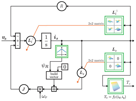
Figure 1. Block diagram of nonlinear current model (CM).

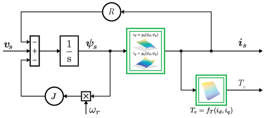
Figure 2. Block diagram of nonlinear flux-linkage model (FLM).

3. Model Parameterization

3.1. Static FEA Batch Simulation

Parameterization of a nonlinear model can be established in two distinct ways, by means of FEA or measurements [32,33]. FEA is preferred when reasonably accurate information about geometry and magnetic characteristics of materials is close at hand, which is especially true for the predesign stage. However, if reliable input data are not at one’s disposal, a systematic measurement procedure can provide fairly accurate parameterization as well [33,34].

Once the designer specifies the magnetostatic finite-element method (FEM) model of IPM, a series of simulations are performed in order to obtain the fundamental electromagnetic relations of the machine. Firstly, the d- and q-axis stator-current vectors with N values over a reasonable range are specified

$${\mathit{I}}_d^{\mathrm{orig}}={\left[I_{d1}\dots I_{dN}\right]}^T{\mathit{I}}_q^{\mathrm{orig}}={\left[I_{q1}\dots I_{qN}\right]}^T.$$

(19)

Then, the batch process iterates over all possible combinations of the d- and q-axis stator currents while performing FEA for each combination. Finally, the batch job returns three matrices ${\mathsf{\Psi }}_d^{\mathrm{orig}}$, ${\mathsf{\Psi }}_q^{\mathrm{orig}}$ and ${\mathit{T}}_{\mathrm{e}}$

$${\mathsf{\Psi }}_d^{\mathrm{orig}}=\left[\begin{array}{ccc}{\mathsf{\Psi }}_{d11}& \dots & {\mathsf{\Psi }}_{d1N}\\ ⋮& \ddots & ⋮\\ {\mathsf{\Psi }}_{dN1}& \dots & {\mathsf{\Psi }}_{dNN}\end{array}\right]{\mathsf{\Psi }}_q^{\mathrm{orig}}=\left[\begin{array}{ccc}{\mathsf{\Psi }}_{q11}& \dots & {\mathsf{\Psi }}_{q1N}\\ ⋮& \ddots & ⋮\\ {\mathsf{\Psi }}_{qN1}& \dots & {\mathsf{\Psi }}_{qNN}\end{array}\right]$$

(20)

$${\mathit{T}}_{\mathrm{e}}=\left[\begin{array}{ccc}{T}_{e11}& \dots & T_{e1N}\\ ⋮& \ddots & ⋮\\ T_{eN1}& \dots & T_{eNN}\end{array}\right]$$

(21)

Matrices ${\mathsf{\Psi }}_d^{\mathrm{orig}}$ and ${\mathsf{\Psi }}_q^{\mathrm{orig}}$ are commonly known as flux-linkage maps, while ${\mathit{T}}_{\mathrm{e}}$ is a torque map. The matrices share the same form with straightforward interpretation: it is a table of numbers that depend on two indices, i and j, which correspond to entries in vectors ${\mathit{I}}_d^{\mathrm{orig}}$ and ${\mathit{I}}_q^{\mathrm{orig}}$, respectively. For example, element ${\mathsf{\Psi }}_{d24}$ gives the value of the d-axis stator flux linkage at specific stator current values ${\mathit{I}}_d^{\mathrm{orig}}\left(2\right)$ and ${\mathit{I}}_q^{\mathrm{orig}}\left(4\right)$.

Figure 3 shows the original flux-linkage maps for an IPM with pronounced nonlinearity than can be visually checked from figures. For example, in case of the d-axis flux linkage (Figure 3a) the surface curvature along d-axis indicates the main saturation, whereas the curvature along the q-axis is indicative of cross-saturation (Figure 3b). Figure 4 shows the electromagnetic torque of the same IPM featuring a curved surface. As expected, the nonlinear effect is more pronounced with higher stator currents in the respective axes.

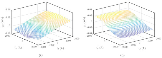
Figure 3. Original flux-linkage map for (a) d-axis and (b) q-axis flux linkage.

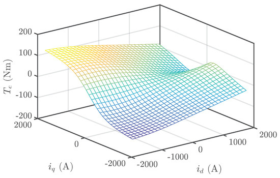
Figure 4. Original torque map for electromagnetic torque.

In this paper, an IPM with data in Table 1 was used as a case study. There are two reasons that all maps are defined for a full (symmetrical) range of currents. The short-circuit test (SCT), which is an important application of the model, is a specific operating state where stator current are not under control. Furthermore, our intention was to illustrate a complete treatment of flux-map inversion. Readers should be aware that, in general, there is no need for a positive $i_d$ current if only a normal IPM operation is considered.

Table 1. Motor data.

Nominal data
Power $P_n$	25 kW
Dc-link voltage $V_{\mathrm{dc}}$	48 V
Maximal phase current $I_{\max }$	778 A
Characteristic current $I_{\mathrm{ch}}$	550 A
Number of pole pairs $p_p$	4
Moment of inertia $\mathsf{\Gamma }$	$0.003$ kgm2
Parameters
Stator resistance $R_s$	$3.3$$\mathrm{m}$$\mathsf{\Omega }$
d-axis inductance $L_d$	$0.013$$\mathrm{m}$H
q-axis inductance $L_q$	$0.029$$\mathrm{m}$H
Rotor flux-linkage ${\mathit{\psi }}_R$	$12.1$ mWb

Flux and torque maps are built for current values ${\mathit{I}}_d^{\mathrm{orig}}={\mathit{I}}_q^{\mathrm{orig}}={[-1860\dots 1860]}^T\mathrm{A}$ in 33 equidistant steps, which results in $33\times 33=1089$ data points. The appropriate range of stator-current values used for flux- and torque-map calculation depends on the specific IPM. In the authors’ experience, the limits should be at least $2.2$ larger than IPM’s maximal current $I_{\max }=778\mathrm{A}$. However, if it turns out that the range is insufficient, reiteration is needed. We also found that further increase in grid density is not justified in light of increasing FE computational costs. An equidistant grid was chosen for convenience.

3.2. CM Parameterization

Once ${\mathsf{\Psi }}_d^{\mathrm{orig}}$, ${\mathsf{\Psi }}_q^{\mathrm{orig}}$, and ${\mathit{T}}_{\mathrm{e}}$ are known for a specific design, it is possible to define their respective interpolation functions $f_d$, $f_q$, and $f_T$:

$${\psi }_d=f_d(i_d,i_q),{\psi }_q=f_q(i_d,i_q),T_e=f_T(i_d,i_q).$$

(22)

CM parameterization requires the calculation of matrices ${\mathit{L}}_s$ and ${\mathit{L}}_i^{-1}$. Because ${\mathit{L}}_i$ is completely oblivious (see Equation (17)), ${\mathit{L}}_i^{-1}$ can be directly calculated using

$${\mathit{L}}_i^{-1}={\left(\frac{\partial {\psi }_d}{\partial i_d}\frac{\partial {\psi }_q}{\partial i_q}-\frac{\partial {\psi }_d}{\partial i_q}\frac{\partial {\psi }_q}{\partial i_d}\right)}^{-1}\left[\begin{array}{cc}\phantom{+}\frac{\partial {\psi }_q}{\partial i_q}& -\frac{\partial {\psi }_d}{\partial i_q}\\ -\frac{\partial {\psi }_q}{\partial i_d}& \phantom{+}\frac{\partial {\psi }_d}{\partial i_d}\end{array}\right],$$

(23)

where an inversion formula for a $2\times 2$ matrix was applied to Equation (13).

On the other hand, apparent inductance matrix ${\mathit{L}}_s$ defined in Equation (11) suffers from major drawback. For example, the first term in ${\mathit{L}}_s$

$$L_{dd}(i_d,i_q)=\frac{{\psi }_d(i_d,i_q)-{\psi }_R(i_d,i_q)}{i_d}$$

besides ${\psi }_d(i_d,i_q)$ also requires ${\psi }_R=f_R(i_d,i_q)$, which is not available from the original set of simulation results. A straightforward solution would be to define ${\psi }_R$ as a constant ${\psi }_R=f_d(0,0)$, but then singularity at $i_d=0$ is unavoidable. Namely, the cross-saturation effect of $i_q$ onto ${\psi }_d$ results in a slight reduction of ${\psi }_d$. In consequence, numerator ${\psi }_d(0,i_q)-{\psi }_R$ does not evaluate to 0, hence resulting in a singularity. A similar reasoning can be adopted for second term $L_{dq}(i_d,i_q)$, where numerator ${\psi }_d(i_d,0)-{\psi }_R\ne 0$ for $i_q=0$.

A practical solution is twofold: neglecting cross-saturation terms in (11)

$${\mathit{L}}_s\left({\mathit{i}}_s\right)=\left[\begin{array}{cc}\frac{{\psi }_d-{\psi }_R}{i_d}& 0\\ 0& \frac{{\psi }_q}{i_q}\end{array}\right]=\left[\begin{array}{cc}{L}_{dd}\left({\mathit{i}}_s\right)& 0\\ 0& L_{qq}\left({\mathit{i}}_s\right)\end{array}\right],$$

(24)

and defining ${\psi }_R=f_d(0,i_q)$ as an explicit function of q-axis current. Then, $L_{dd}$ can be calculated for all current combinations without incurring a singularity

$$L_{dd}(i_d,i_q)=\frac{{\psi }_d(i_d,i_q)-{\psi }_d(0,i_q)}{i_d}.$$

It is clear from the above argument that parameterization with the original set of FEA data requires CM simplification. Whether its impact is considerable or marginal depends on the grade of nonlinearity of the particular machine. Machines with pronounced nonlinearity, as is the case for IPMs, may therefore require a full inductance matrix. At this point, it should be mentioned that approaches that can overcome the limits in calculating original Equation (11) were reported, e.g., frozen-permeances method. However, this technique requires an additional FEA set, effectively doubling the computational burden.

3.3. FLM Parameterization

In comparison to CM, FLM simulation form Equation (18) is simpler, as only matrix ${\mathit{F}}_s$ has to be parameterized. Even though the four terms in ${\mathit{F}}_s$ are elementary ratios of the stator current and flux linkage, e.g., a first term in Equation (15)

$$F_{dd}({\psi }_d,{\psi }_q)=\frac{i_d({\psi }_d,{\psi }_q)}{{\psi }_d},$$

they cannot be readily calculated using previously defined functions $f_d$ and $f_q$. The underlying reason is that the simulation flow of FLM treats flux linkage as the independent variable as far as current-flux relation is concerned. Therefore, an inverse relation between current and flux linkage must be determined beforehand. Drawing an analogy between CM and FLM, we define corresponding interpolating functions

$$i_d=g_d({\psi }_d,{\psi }_q),i_q=g_q({\psi }_d,{\psi }_q).$$

(25)

The relation between two sets of interpolating Functions (22) and (25) can be thought of as a mathematical inverse of two variate functions

$$\begin{array}{cc}\hfill i_d& =g_d(f_d(i_d,i_q),f_q(i_d,i_q))\hfill \end{array}$$

(26)

$$\begin{array}{cc}\hfill i_q& =g_q(f_d(i_d,i_q),f_q(i_d,i_q)).\hfill \end{array}$$

(27)

An important question to be answered is whether inverse functions $g_d$ and $g_q$ actually exist. Consider mapping $f:{\mathbf{R}}^2\to {\mathbf{R}}^2$, defined by

$$f(i_d,i_q)=\left[\begin{array}{c}{f}_d(i_d,i_q)\\ f_q(i_d,i_q)\end{array}\right].$$

(28)

If the derivative of a mapping f is invertible at some point $(i_{\mathrm{d}0},i_{\mathrm{q}0})$, then mapping f is locally invertible in some neighborhood of point $f(i_{\mathrm{d}0},i_{\mathrm{q}0})$ [35]. The derivative of f is just a Jacobian matrix

$${\mathit{J}}_f=\left[\begin{array}{cc}\frac{\partial f_d}{\partial i_d}& \frac{\partial f_d}{\partial i_q}\\ \frac{\partial f_q}{\partial i_d}& \frac{\partial f_q}{\partial i_q}\end{array}\right],$$

(29)

which is invertible exactly when its determinant is nonzero:

$$\mathbf{det}\left({\mathit{J}}_f\right)=\frac{\partial f_d}{\partial i_d}\frac{\partial f_q}{\partial i_q}-\frac{\partial f_d}{\partial i_q}\frac{\partial f_q}{\partial i_d}\ne 0.$$

(30)

Mapping f is invertible over the domain of current vectors ${\mathit{I}}_d^{\mathrm{orig}}$ and ${\mathit{I}}_q^{\mathrm{orig}}$ only if the corresponding $\mathbf{det}\left({\mathit{J}}_f\right)$ is strictly nonzero at every point in the domain. Figure 5 shows the Jacobian determinant for the IPM in question (see Table 1). For this particular machine, it is clear that the determinant is strictly positive; therefore, the IPM’s flux maps are invertible over the whole domain.

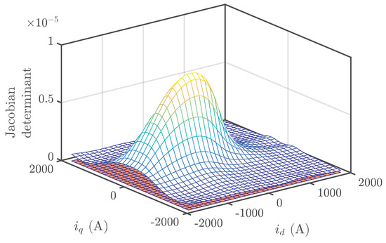
Figure 5. Jacobian determinant ${\mathit{J}}_f$ over the domain of current vectors ${\mathit{I}}_d^{\mathrm{orig}}$ and ${\mathit{I}}_q^{\mathrm{orig}}$.

It is interesting to inspect Equation (30) more closely in order to gain some insight in its behavior for a general machine. The first term is always strictly positive, as $f_d$ and $f_q$ are both monotone-increasing, which can easily be seen by inspection. This property is also physically sound because increasing the current always results in increased flux linkage in the respective axis. The inspection of the second term is more involved, but careful analysis shows that it is also strictly positive, as can be seen in Figure 6. For this reason, the first term must always be bigger than the second so as to maintain invertible mapping f. If we associate the two terms with main and cross magnetization, respectively, we can see that this is an entirely reasonable expectation for a practical machine. Typically, the level of main magnetization is about one order of magnitude higher than that of cross-magnetization.

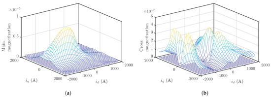
Figure 6. (a) Main and (b) cross-magnetization term in equation for Jacobian determinant. Note the different order of magnitude.

If interpolation functions $g_d$ and $g_q$ exist, they can be found in various ways. In accordance to Equation (19), we generate d- and q-axis stator flux-linkage vectors with N-equidistant, monotone-increasing entries

$${\mathsf{\Psi }}_d^{\mathrm{new}}={\left[{\mathsf{\Psi }}_{d1}\dots {\mathsf{\Psi }}_{dN}\right]}^T{\mathsf{\Psi }}_q^{\mathrm{new}}={\left[{\mathsf{\Psi }}_{q1}\dots {\mathsf{\Psi }}_{qN}\right]}^T,$$

where their range is specified by the minimal and maximal value of original maps ${\mathsf{\Psi }}_d^{\mathrm{orig}}$ and ${\mathsf{\Psi }}_d^{\mathrm{orig}}$, respectively.

3.3.1. Inversion via Minimization

One way to find inverse maps ${\mathit{I}}_d^{\mathrm{new}}$ and ${\mathit{I}}_q^{\mathrm{new}}$ is to minimize the residual between interpolation points and the value of interpolating function over whole set $i,j=1\dots N$. This translates to a multiobjective nonlinear least-squares problem with two objectives, one for each component

$$\begin{array}{cc}\hfill J_{d,ij}(i_d,i_q)& =\left|\right|{\mathsf{\Psi }}_d^{\mathrm{new}}\left(i\right)-f_d(i_d,i_q){\left|\right|}^2\hfill \\ \hfill J_{q,ij}(i_d,i_q)& =\left|\right|{\mathsf{\Psi }}_q^{\mathrm{new}}\left(j\right)-f_q(i_d,i_q){\left|\right|}^2.\hfill \end{array}$$

For each iteration, a unique solution $(i_d^{\mathrm{sol}},i_q^{\mathrm{sol}})$ exists, which is interpreted as an entry in inverse maps ${\mathit{I}}_d^{\mathrm{new}}(i,j)=i_d^{\mathrm{sol}}$ and ${\mathit{I}}_q^{\mathrm{new}}(i,j)=i_q^{\mathrm{sol}}$. Formally, we can express the idea as

$$\mathrm{minimize}\left|\right|r_{ij}(i_d,i_q){\left|\right|}^2,$$

(31)

where the residual is defined as $r_{ij}(i_d,i_q)=J_{d,ij}(i_d,i_q)+J_{q,ij}(i_d,i_q)$. Once inverse maps ${\mathit{I}}_d^{\mathrm{new}}$ and ${\mathit{I}}_q^{\mathrm{new}}$ are obtained, one can easily define interpolation functions $g_d$ and $g_d$.

3.3.2. Inversion via Intersections

An equivalent solution for determining inverse maps ${\mathit{I}}_d^{\mathrm{new}}$ and ${\mathit{I}}_q^{\mathrm{new}}$ is via intersections. Original maps ${\mathsf{\Psi }}_d^{\mathrm{orig}}$ and ${\mathsf{\Psi }}_q^{\mathrm{orig}}$ are first interpolated (functions $f_d$ and $f_q$) and then sliced into predefined number of contour isolines at flux-linkage levels ${\mathsf{\Psi }}_d^{\mathrm{new}}\left(i\right)$ or ${\mathsf{\Psi }}_d^{\mathrm{new}}\left(j\right)$. These lines can be interpreted as curves in the current co-ordinates, where each of these curves encodes all possible combinations $(i_d,i_q)$ for a particular flux-linkage level. Algorithm 1 then proceeds to find an intersection between curves at ${\mathsf{\Psi }}_d^{\mathrm{new}}\left(i\right)$ and ${\mathsf{\Psi }}_q^{\mathrm{new}}\left(j\right)$ for all combinations of the stator flux-linkage. If Condition (30) holds, then a unique intersection exists for each pair of ${\mathsf{\Psi }}_d^{\mathrm{new}}\left(i\right)$ and ${\mathsf{\Psi }}_q^{\mathrm{new}}\left(j\right)$. These solutions are not only more intuitive due to a clear geometrical interpretation, but also significantly faster.

Algorithm 1 Inverse flux map via intersection.

1: Define number of flux isolines n (levels) 2: Slice flux map ${\psi }_d=f_d(i_d,i_q)$ (3D) into n isolines (2D) 3: Slice flux map ${\psi }_q=f_q(i_d,i_q)$ (3D) into n isolines (2D) 4: Obtain $2n$ isolines ${\psi }_{d,i}$ and ${\psi }_{q,j}$ 5: Initialize empty $n\times n$ matrices ${\mathsf{\Psi }}_d^{\mathrm{new}}$, ${\mathsf{\Psi }}_q^{\mathrm{new}}$, ${\mathit{I}}_d^{\mathrm{new}}$, and ${\mathit{I}}_q^{\mathrm{new}}$ 6: for$i\leftarrow 1\dots n$do 7:    for $j\leftarrow 1\dots n$ do 8:       Find intersection ($x_d,x_q$) between ${\psi }_{d,i}$ and ${\psi }_{q,j}$ 9:       Update ${\mathsf{\Psi }}_d^{\mathrm{new}}(i,j)={\psi }_{d,i}$ and ${\mathsf{\Psi }}_q^{\mathrm{new}}(i,j)={\psi }_{q,j}$ 10:       Update ${\mathit{I}}_d^{\mathrm{new}}(i,j)=x_d$ and ${\mathit{I}}_d^{\mathrm{new}}(i,j)=x_q$ 11:    end for 12: end for 13: Extrapolate ${\mathit{I}}_d^{\mathrm{new}}$ and ${\mathit{I}}_q^{\mathrm{new}}$ at corners 14: return${\mathsf{\Psi }}_d^{\mathrm{new}}$, ${\mathsf{\Psi }}_q^{\mathrm{new}}$, ${\mathit{I}}_d^{\mathrm{new}}$, and ${\mathit{I}}_q^{\mathrm{new}}$

Figure 7 shows the resulting inverse flux maps using the intersection algorithm. In order to validate inversion accuracy, flux-linkage errors

$$\begin{array}{cc}\hfill {\Delta }_d& =f_d(g_d({\psi }_d,{\psi }_q),g_q({\psi }_d,{\psi }_q))-{\psi }_d\hfill \end{array}$$

(32)

$$\begin{array}{cc}\hfill {\Delta }_q& =f_q(g_d({\psi }_d,{\psi }_q),g_q({\psi }_d,{\psi }_q))-{\psi }_q\hfill \end{array}$$

(33)

are checked for the whole range of flux-linkage values. For each flux-linkage pair $({\psi }_d,{\psi }_q)$, their respective currents $(i_d,i_q)$ are calculated using interpolating functions $g_d$ and $g_q$. Then, these currents are plugged into $f_d$ and $f_q$, resulting in a new flux-linkage pair that should be as close as possible to the original. Figure 8 confirms that the maximum error did not exceed 0.1% in either axis.

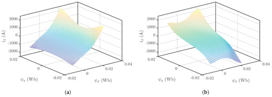
Figure 7. Inverse flux map for (a) d-axis and (b) q-axis current.

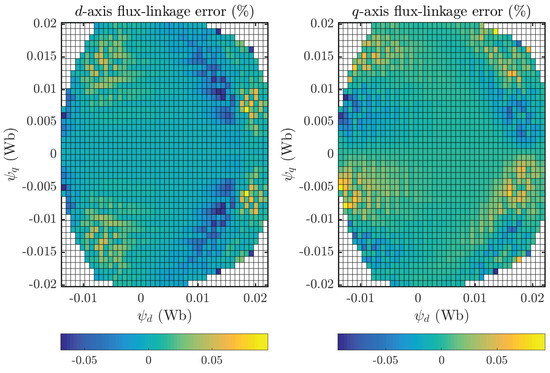
Figure 8. Flux-linkage error for (Left) d-axis and (Right) q-axis.

4. CM and FLM Performance Comparison

4.1. Model Verification

First, we compare the performance of CM and FLM in a dynamic simulation. A three-phase short-circuit test (SCT), a well-established IPM test procedure in the industry [36], was chosen because high transient currents were expected to push the IPM deep into saturation. In this way, both models could conveniently be assessed in terms of nonlinearity. The chosen IPM (Table 1) is intended for small urban electric vehicles. As the IPM nominal voltage level was low ($V_{\mathrm{dc}}=48 \mathrm{V}$), the maximal current was rather large $I_{\max }=778 \mathrm{A}$. Both inductances were valid for a nominal operation point.

During the SCT, the IPM rotor is driven by an external machine at a constant speed, when stator windings (at first open) are suddenly short-circuited. Figure 9 depicts the stator currents in $dq$ co-ordinates for CM and FLM. There was practically a perfect match between currents, the sole difference being a slightly higher oscillation frequency for CM. One can conclude that CM and FLM are equivalent in terms of performance.

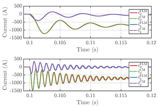
Figure 9. Comparison of FLM and CM for a three-phase symmetric short circuit at (top) 3000 min⁻¹ and (bottom) 15,000 min${}^{-1}$.

Then, FLM simulation results of a three-phase SCT were compared to measurements on a prototype machine (Figure 10). The time-domain response of the phase currents to the sudden short circuit depends on the starting position of the rotor. In order to compare measurements with simulations, the time traces of phase currents must be synchronized. Unfortunately, the measurement setup did not allow to choose the exact instant of the short-circuit maneuver. Therefore, the measurement was performed first and the appropriate time instant of the short circuit in simulation was determined afterwards. It is noteworthy to observe that FLM is capable or forecasting true maximal phase current (in this case red signal at $t=0.013 \mathrm{s}$).

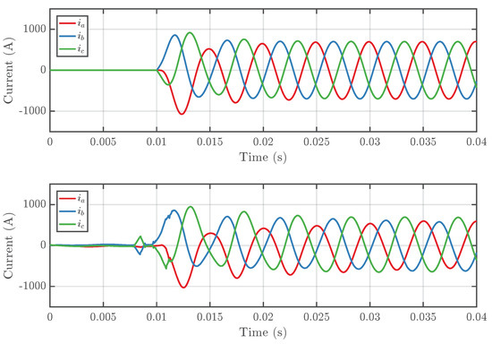
Figure 10. Three-phase short circuit at 3000 min⁻¹: (top) simulations and (bottom) measurements.

Nevertheless, a direct comparison of individual phase currents (Figure 11) reveals discrepancies between measurement and simulation. All three measured phase currents had smaller peak-to-peak values, which can be attributed to nonzero contact resistance. The DC component in measurements died out slower than predicted by the simulations.

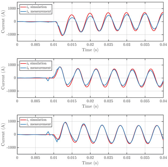
Figure 11. Three-phase short circuit at 3000 min⁻¹: a direct comparison of simulated and measured phase currents (top) $i_a$, (middle) $i_b$, and (bottom) $i_c$.

4.2. Parameterization Time

CM and FLM were implemented in Matlab/Simulink and run on a typical workstation with $3.40$ GHz and 16 GB RAM. Even though both models were parameterized with the same input data, the process itself differed. CM parameterization includes the calculation of interpolation functions for the inverse of incremental inductance, apparent inductance, and rotor flux linkage. On the other hand, the FLM requires an inversion of flux maps and subsequent determination of interpolation functions. Parameterization time denotes the computational time required for full-model parameterization before the simulation can be actually run. Table 2 shows that, in the case of FLM parameterization, the proposed intersection method is superior to the minimization method by an order of magnitude. The FLM parameterization time is thus comparable to CM, even though the latter still performs twice faster. However, the said differences fade completely, as execution time of simulation is nearly always significantly longer.

Table 2. Comparison of parameterization times.

Model Type	Parameterization Time
CM	$0.24$ s
FLM via intersections	$0.49$ s
FLM via minimization	$58.0$ s

4.3. Execution Time

Next, we compared the performance of the CM and FLM in terms of their execution time. Two rather basic simulation tasks were chosen as examples: three-phase short-circuit and full acceleration from standstill to deep field weakening, where the motor model is part of the speed control loop. The real-time time frame of the latter task was set at 10 s. The results in Table 3 clearly show that the FLM was faster than CM in both cases. It is interesting to note that, in terms of the control loop simulation, the FLM has a considerable margin of almost 20% over CM.

Table 3. Comparison of execution times.

Simulation Task	FLM	CM	Improvement
Three-phase short circuit	$12.5$ s	$13.8$ s	9.4%
Control with field weakening	$34.6$ s	$42.4$ s	18.4%
Demagnetization risk assessment	375 min	414 min	9.4%
WLTC driving cycle	104 min	127 min	18.1%

As there are numerous possible situations for which dynamical simulations are typically performed, we particularly focused on scenarios where significant computational effort is inevitable. We were interested in the question of whether time-consuming tasks could be significantly reduced by using the FLM instead of CM. Two computationally intensive simulation tasks with high practical value were chosen as representative scenarios: (a) assessment of demagnetization risk during a three-phase short circuit and (b) WLTC driving cycle. The computational effort of the former scenario stems from an excessive number of iterations. In contrast, the latter scenario demands comparatively a long real-time time frame of 30 min. It should be added that both scenarios require only one parameterization at the beginning.

The assessment of demagnetization risk during a three-phase short circuit requires many iterations of the basic three-phase short-circuit for different operating points $(T,n)$ in the torque-speed diagram. Every steady-state operating point $(T,n)$ is associated with the specific value of $I_d$ (Figure 12) and $I_q$ (not shown). Here, the torque-speed diagram contains $30\times 60=1800$ operating points. Each current pair $(I_d,I_q)$ is fed as an initial value $(I_d^{\mathrm{init}},I_q^{\mathrm{init}})=(I_d,I_q)$ into the space-state model, which calculates respective transient short-circuit currents $i_d\left(t\right)$ and $i_q\left(t\right)$. For example, Figure 13 depicts transient for 9 operation point (56 Nm, 5000 min⁻¹). The critical time instant $t_{\mathrm{crit}}$, where d-axis current reaches its global negative peak, is determined by

$$t_{\mathrm{crit}}=\underset{t}{\arg \min }{i}_d\left(t\right).$$

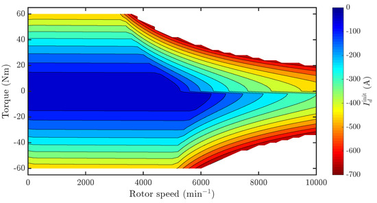
Figure 12. Initial current $I_d^{\mathrm{init}}$ for a three-phase short circuit.

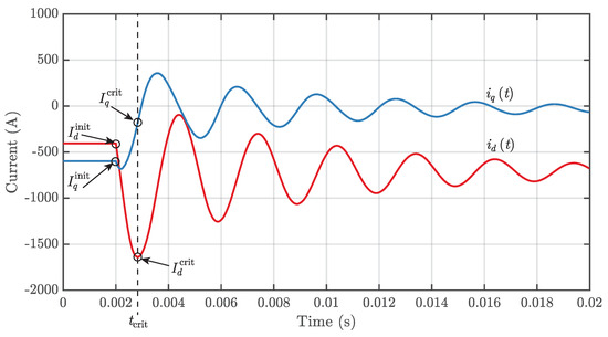
Figure 13. Three-phase short circuit for worst-case operation point (56 Nm, 5000 min⁻¹), where $I_d^{\mathrm{init}}=-405 \mathrm{A}$ and $I_q^{\mathrm{init}}=-599 \mathrm{A}$.

The negative peak value of d-axis current $I_d^{\mathrm{crit}}=i_d\left(t_{\mathrm{crit}}\right)$ and the coincidental q-axis current $I_q^{\mathrm{trans}}=i_q\left(t_{\mathrm{crit}}\right)$ are then identified and stored (Figure 13). In this way, a complete prediction of $(I_d^{\mathrm{crit}},I_q^{\mathrm{crit}})$ for the whole torque-speed diagram is obtained.

The d-axis current $I_d^{\mathrm{crit}}$ is the worst-case instantaneous value for specific operating point $(T,n)$ and is directly associated with demagnetization risk. Figure 14 depicts the predicted $I_d^{\mathrm{crit}}$ for the torque-speed diagram. We can observe that the highest negative values of $I_d^{\mathrm{crit}}$ are expected when the IPM is delivering peak power (big $i_q$). It is interesting to note that there is less of a demagnetization risk when the machine operates in deep flux weakening. Moreover, the $I_d^{\mathrm{crit}}$ in generating mode is larger than its counterpart in motoring mode.

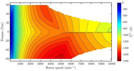
Figure 14. Peak transient current $I_d^{\mathrm{crit}}$ for three-phase short circuit.

Operating points, where values of $I_d^{\mathrm{crit}}$ are critically low, are identified as candidates for demagnetization. Therefore, precise re-evaluation of this operating point with FEA was performed. The corresponding current pair $(I_d^{\mathrm{crit}},I_q^{\mathrm{crit}})$ is fed into the magnetostatic simulation. Precise calculation of the magnetic field inside magnets enables reliable demagnetization risk assessment.

As this particular scenario is a simple iteration of the basic simulation task described above, we could estimate the execution time for both models. The FLM enabled 9.4% faster execution in comparison to CM, which can be considered a significant improvement (Table 3).

The torque-speed diagram in Figure 12 and Figure 14 requires comment. The envelope of the diagram is not symmetrical for motoring (top) and generating (bottom), as the transition speed between a constant torque operation and flux-weakening operation differs for motoring and generating mode, which is mainly due to the 48 V car battery being used as a DC source. A significant relative difference in bus voltage for motoring (48 V) and generating (52 V) mode is further aggravated by the effect of losses and stator resistance, which explains the difference in the torque-speed envelope.

Analogously, the WLTC driving cycle scenario is very similar to another basic simulation task described above, namely, control with field weakening. WLTC prescribes speed values for each second in the 30 min time frame. Consequently, the time series of speed values is treated as a reference for the control loop drive. As we can observe from Table 3, the FLM-based simulation model was 18.1% faster than its counterpart.

5. Conclusions

In this paper, an FEM-parameterized two-axis model of IPM was thoroughly analyzed, and its two implementations (i.e., CM and FLM) were compared from the point of view of accuracy and computational demand. Since parameterization of FLM involves the inversion of flux maps, it is mathematically more complex than analog CM tasks, thus resulting in significantly higher computational and, by extension, time demand. For this reason, a procedure for fast and reliable parameterization FLM was presented. The proposed procedure is one order of magnitude faster than the comparable methods, hence providing considerable improvement in terms of computational time. In this way, the major drawback of using FLM were overcome. It was established that the error of the inversion process was under 0.02%.

Additionally, we showed that the execution time of FLM was up to 20% shorter in comparison to CM. As the parameterization time of FLM is now comparable to CM, we strongly advocate the use of FLM in computationally intensive simulation scenarios, which include a significant number of iterations or have an excessive time span. This is why FLM should be used in the Hardware-in-the-Loop experiment platform as well, since the real-time computational burden should be as low as possible.

References

- EL-Refaie, A.M. Fractional-Slot Concentrated-Windings Synchronous Permanent Magnet Machines: Opportunities and Challenges. IEEE Trans. Ind. Electron. 2010, 57, 107–121. [Google Scholar] [CrossRef]
- Hu, Y.; Zhu, S.; Liu, C.; Wang, K. Electromagnetic Performance Analysis of Interior PM Machines for Electric Vehicle Applications. IEEE Trans. Energy Convers. 2018, 33, 199–208. [Google Scholar] [CrossRef]
- Carraro, E.; Bianchi, N. Design and comparison of interior permanent magnet synchronous motors with non-uniform airgap and conventional rotor for electric vehicle applications. IET Electr. Power Appl. 2014, 8, 240–249. [Google Scholar] [CrossRef]
- Pellegrino, G.; Vagati, A.; Guglielmi, P.; Boazzo, B. Performance Comparison Between Surface-Mounted and Interior PM Motor Drives for Electric Vehicle Application. IEEE Trans. Ind. Electron. 2012, 59, 803–811. [Google Scholar] [CrossRef]
- Torrent, M.; Perat, J.I.; Jiménez, J.A. Permanent Magnet Synchronous Motor with Different Rotor Structures for Traction Motor in High Speed Trains. Energies 2018, 11. [Google Scholar] [CrossRef]
- Pellegrino, G.; Jahns, T.M.; Bianchi, N.; Soong, W.; Cupertino, F. The Rediscovery of Synchronous Reluctance and Ferrite Permanent Magnet Motors: Tutorial Course Notes; Springer: Basel, Switzerland, 2016. [Google Scholar] [CrossRef]
- Germishuizen, J.J.; Kamper, M.J. IPM Traction Machine With Single Layer Non-Overlapping Concentrated Windings. IEEE Trans. Ind. Appl. 2009, 45, 1387–1394. [Google Scholar] [CrossRef]
- Germishuizen, J.J.; Stanton, S.; Delafosse, V. Integrating FEM in an everyday design environment to accurately calculate the performance of IPM motors. In Proceedings of the 2009—XIV International Symposium on Electromagnetic Fields in Mechatronics, Electrical and Electronic Engineering (ISEF), Arras, France, 10–12 September 2009. [Google Scholar]
- Li, L.; Li, W.; Li, D.; Li, J.; Fan, Y. Research on Strategies and Methods Suppressing Permanent Magnet Demagnetization in Permanent Magnet Synchronous Motors Based on a Multi-Physical Field and Rotor Multi-Topology Structure. Energies 2018, 11. [Google Scholar] [CrossRef]
- Liu, X.; Lin, Q.; Fu, W. Optimal Design of Permanent Magnet Arrangement in Synchronous Motors. Energies 2017, 10, 1700. [Google Scholar] [CrossRef]
- Liu, Y.X.; Li, L.Y.; Cao, J.W.; Gao, Q.H.; Sun, Z.Y.; Zhang, J.P. The Optimization Design of Short-Term High-Overload Permanent Magnet Motors Considering the Nonlinear Saturation. Energies 2018, 11, 3272. [Google Scholar] [CrossRef]
- Pries, J.; Burress, T. High fidelity D-Q modeling of synchronous machines using spectral interpolation. In Proceedings of the 2017 IEEE Transportation Electrification Conference and Expo (ITEC), Chicago, IL, USA, 26–28 June 2017; pp. 779–785. [Google Scholar] [CrossRef]
- Alvarez-Gonzalez, F.; Griffo, A.; Sen, B.; Wang, J. Real-Time Hardware-in-the-Loop Simulation of Permanent-Magnet Synchronous Motor Drives Under Stator Faults. IEEE Trans. Ind. Electron. 2017, 64, 6960–6969. [Google Scholar] [CrossRef]
- Zhang, C.; Guo, Q.; Li, L.; Wang, M.; Wang, T. System Efficiency Improvement for Electric Vehicles Adopting a Permanent Magnet Synchronous Motor Direct Drive System. Energies 2017, 10, 2030. [Google Scholar] [CrossRef]
- Krause, P.; Wasynczuk, O.; Sudhoff, S.; Pekarek, S. Analysis of Electric Machinery and Drive Systems; Wiley-IEEE Press: Hoboken, NJ, USA, 2013. [Google Scholar]
- Vas, P. Electrical Machines and Drives: A Space-Vector Theory Approach; Clarendon Press: Oxford, UK, 1993. [Google Scholar]
- Štumberger, B.; Štumberger, G.; Dolinar, D.; Hamler, A.; Trlep, M. Evaluation of saturation and cross-magnetization effects in interior permanent-magnet synchronous motor. IEEE Trans. Ind. Appl. 2003, 39, 1264–1271. [Google Scholar] [CrossRef]
- Chen, X.; Wang, J.; Sen, B.; Lazari, P.; Sun, T. A High-Fidelity and Computationally Efficient Model for Interior Permanent-Magnet Machines Considering the Magnetic Saturation, Spatial Harmonics, and Iron Loss Effect. IEEE Trans. Ind. Electron. 2015, 62, 4044–4055. [Google Scholar] [CrossRef]
- Boesing, M.; Niessen, M.; Lange, T.; Doncker, R.D. Modeling spatial harmonics and switching frequencies in PM synchronous machines and their electromagnetic forces. In Proceedings of the 2012 XXth International Conference on Electrical Machines, Marseille, France, 2–5 September 2012; pp. 3001–3007. [Google Scholar] [CrossRef]
- Weidenholzer, G.; Silber, S.; Jungmayr, G.; Bramerdorfer, G.; Grabner, H.; Amrhein, W. A flux-based PMSM motor model using RBF interpolation for time-stepping simulations. In Proceedings of the 2013 International Electric Machines Drives Conference, Chicago, IL, USA, 12–15 May 2013; pp. 1418–1423. [Google Scholar] [CrossRef]
- Pinto, D.E.; Pop, A.C.; Kempkes, J.; Gyselinck, J. dq0-modeling of interior permanent-magnet synchronous machines for high-fidelity model order reduction. In Proceedings of the 2017 International Conference on Optimization of Electrical and Electronic Equipment (OPTIM) 2017 Intl Aegean Conference on Electrical Machines and Power Electronics (ACEMP), Fundata, Romania, 25–27 May 2017; pp. 357–363. [Google Scholar] [CrossRef]
- Luo, G.; Zhang, R.; Chen, Z.; Tu, W.; Zhang, S.; Kennel, R. A Novel Nonlinear Modeling Method for Permanent-Magnet Synchronous Motors. IEEE Trans. Ind. Electron. 2016, 63, 6490–6498. [Google Scholar] [CrossRef]
- Fasil, M.; Antaloae, C.; Mijatovic, N.; Jensen, B.B.; Holboll, J. Improved dq-Axes Model of PMSM Considering Airgap Flux Harmonics and Saturation. IEEE Trans. Appl. Supercond. 2016, 26, 1–5. [Google Scholar] [CrossRef]
- Li, S.; Han, D.; Sarlioglu, B. Modeling of Interior Permanent Magnet Machine Considering Saturation, Cross Coupling, Spatial Harmonics, and Temperature Effects. IEEE Trans. Transp. Electrif. 2017, 3, 682–693. [Google Scholar] [CrossRef]
- Stipetić, S.; Goss, J.; Žarko, D.; Popescu, M. Calculation of Efficiency Maps Using a Scalable Saturated Model of Synchronous Permanent Magnet Machines. IEEE Trans. Ind. Appl. 2018, 54, 4257–4267. [Google Scholar] [CrossRef]
- Chu, W.Q.; Zhu, Z.Q. Average Torque Separation in Permanent Magnet Synchronous Machines Using Frozen Permeability. IEEE Trans. Magn. 2013, 49, 1202–1210. [Google Scholar] [CrossRef]
- Dück, P.; Ponick, B. A novel iron-loss-model for permanent magnet synchronous machines in traction applications. In Proceedings of the 2016 International Conference on Electrical Systems for Aircraft, Railway, Ship Propulsion and Road Vehicles International Transportation Electrification Conference (ESARS-ITEC), Toulouse, France, 2–4 November 2016; pp. 1–6. [Google Scholar] [CrossRef]
- Mellor, P.H.; Wrobel, R.; Holliday, D. A computationally efficient iron loss model for brushless AC machines that caters for rated flux and field weakened operation. In Proceedings of the 2009 IEEE International Electric Machines and Drives Conference, Miami, FL, USA, 3–6 May 2009; pp. 490–494. [Google Scholar] [CrossRef]
- Bramerdorfer, G.; Andessner, D. Accurate and Easy-to-Obtain Iron Loss Model for Electric Machine Design. IEEE Trans. Ind. Electron. 2017, 64, 2530–2537. [Google Scholar] [CrossRef]
- Miller, T.J.E.; Popescu, M.; Cossar, C.; McGilp, M. Performance estimation of interior permanent-magnet brushless motors using the voltage-driven flux-MMF diagram. IEEE Trans. Magn. 2006, 42, 1867–1872. [Google Scholar] [CrossRef]
- Bianchi, N.; Alberti, L. MMF Harmonics Effect on the Embedded FE Analytical Computation of PM Motors. IEEE Trans. Ind. Appl. 2010, 46, 812–820. [Google Scholar] [CrossRef]
- Liu, K.; Feng, J.; Guo, S.; Xiao, L.; Zhu, Z.Q. Identification of Flux Linkage Map of Permanent Magnet Synchronous Machines Under Uncertain Circuit Resistance and Inverter Nonlinearity. IEEE Trans. Ind. Inf. 2018, 14, 556–568. [Google Scholar] [CrossRef]
- Armando, E.; Bojoi, R.; Guglielmi, P.; Pellegrino, G.; Pastorelli, M. Experimental methods for synchronous machines evaluation by an accurate magnetic model identification. In Proceedings of the 2011 IEEE Energy Conversion Congress and Exposition, Phoenix, AZ, USA, 17–22 September 2011; pp. 1744–1749. [Google Scholar] [CrossRef]
- Marčič, T.; Štumberger, G.; Štumberger, B. Analyzing the Magnetic Flux Linkage Characteristics of Alternating Current Rotating Machines by Experimental Method. IEEE Trans. Magn. 2011, 47, 2283–2291. [Google Scholar] [CrossRef]
- Hubbard, J.H.; Burke Hubbard, B. Vector Calculus, Linear Algebra, and Differential Forms: A Unified Approach; Prentice Hall: Upper Saddle River, NJ, USA, 1998. [Google Scholar]
- Choi, G.; Jahns, T.M. Investigation of Key Factors Influencing the Response of Permanent Magnet Synchronous Machines to Three-Phase Symmetrical Short-Circuit Faults. IEEE Trans. Energy Convers. 2016, 31, 1488–1497. [Google Scholar] [CrossRef]
© 2019 by the authors. Licensee MDPI, Basel, Switzerland. This article is an open access article distributed under the terms and conditions of the Creative Commons Attribution (CC BY) license (http://creativecommons.org/licenses/by/4.0/).