Enhanced Flat Window-Based Synchrophasor Measurement Algorithm for P Class PMUs

Abstract

Accurate and fast synchrophasor measurement, especially under dynamics and distortions, is crucial for control and protection of power grid. The dynamics and distortions in the power grid may occur simultaneously, which increase the complexity of the problem. To address this issue, an enhanced flat window-based P class synchrophasor measurement algorithm (EFW-PSMA) is proposed in this paper. Firstly, an EFW is design based on the least square (LS) approach. Secondly, the EFWs are adopted as the low pass filters (LPFs) in the EFW-PSMA structure to extract the fundamental component. Finally, the frequency and rate of change of frequency (ROCOF) are estimated based on the LS approach. The EFW-PSMA has a simple implementation structure and low computation complexity. Theoretical analysis and simulation results verify the superiority of the method, especially under stressed grid conditions, where several types of disturbances occur simultaneously. The maximum total vector error (TVE) is 0.3% under the most stressed conditions that all the disturbances specified in the benchmark tests specified in the IEC/IEEE 60255-118-1 occur simultaneously. It means that the EFW-PSMA could be used for the protection applications of the synchrophasor measurement algorithm, which is important for PMUs to fast response in the control and protection actions in order to avert a possible collapse or other abnormal conditions.

1. Introduction

Phase measurement units (PMUs) are widely deployed for power systems network monitoring in real time. PMU applications in wide-area measurement systems (WAMS) are highly affected by their synchrophasor measurement algorithm (SMA). Fast and robust SMA is crucial for the fast response in the control and protection actions in order to avert a possible collapse or other abnormal conditions [1,2].

In IEC/IEEE 60255-118-1 [3], the SMAs are classified into P class (PSMA) and M class (MSMA) due to their different applications in the power applications. PSMA is mainly for the protection applications, and MSMA is mainly for the monitoring applications. Different benchmark tests and measurement accuracy requirements are mandated for each class. Compared with the MSMA, the PSMA needs a much faster response, which means a limitation of data window length and special filters in the PSMA structure. Thus, the PSMA should be designed carefully to obtain both a fast-dynamic response and a satisfying disturbance rejection capability.

The popular PSMAs include the discrete fourier transform (DFT)-based methods [4,5,6,7,8,9,10,11], demodulation [12], Kalman filter [13,14], least squares [15,16], wavelet transform [17,18], level crossing [19], subspace algorithm [20], neural network [21], Newton algorithm [22], phase-locked loop (PLL) [23], etc. Some papers prove the effectiveness of the aforementioned methods, such as the DFT-based method having good harmonics rejection and low computation burden, so it can be implemented simply by hardware. However, due to the scalloping loss caused by the main lobe of the Fourier filter, the main drawback of the DFT-based method is the performance at off-nominal frequency. Phase-locked loop-based methods have simple construers and good response performance, but there is a tradeoff between the disturbance rejection capability and the dynamic response speed.

To regulate the performance of the PSMAs, the benchmark tests and measurement accuracy requirements under dynamics and distortions are given and specified in the IEC/IEEE 60255-118-1. The benchmark tests are focused on the PSMAs’ behavior under different types of disturbances, particularly in the presence of frequency deviation, harmonics distortions, dynamics including amplitude/phase modulation and frequency ramp. According to IEC/IEEE 60255-118-1, the total vector error (TVE) associated with phasor measurement must be smaller than or equal to 1% in steady-state conditions and 3% in dynamic conditions. The majority of the exiting PSMAs satisfy the measurement accuracy requirements in the benchmark. However, most of the studies have focused on the methods’ behavior under single type of disturbance. Yet in practice, several types of disturbance may occur simultaneously. For example, frequency deviation, harmonics distortions and power swing may occur simultaneously. The phasor estimation accuracy during these stressed conditions is vital for system stability.

The synchrophasor measurement under stressed conditions that several disturbances occur simultaneously has attracted more attention recently. A Clarke transformation-based phasor algorithm is proposed in [9] which considered harmonics distortions and frequency deviation in the meantime. A modified dynamic synchrophasor estimation algorithm is proposed in [24], which considers power oscillation and frequency deviation in the meantime. The frequency feedback branch is adopted in the method to improve the phasor estimation accuracy. The corresponding coefficient against the different frequency estimations is applied to the dynamic phasor estimator to yield accurate synchrophasor estimation with the consideration of large frequency deviation. The results show that the proposed algorithm can get more accurate phasor estimations than our previous work most of the time with the cost of a minor increase of computational power. An accurate dynamic phasor estimation method is proposed in [25]. This method uses the signal model under these dynamic conditions, linearize them by using Taylor’s series expansion, and estimate the phasor using least squares technique which considers frequency deviation and power oscillation without the frequency feedback branch. The optimal window-based SMA is studied in [26], which considers frequency deviation and harmonics in the meantime and it is shown that most of the performance requirements specified in the standard can be satisfied with a proper selection of the algorithm characteristics. However, the more stressed conditions, such as frequency deviation, harmonic distortions and power oscillation occurs simultaneously, may give forth to large errors in these methods.

To solve the aforementioned issue, an enhanced flat window-based PSMA (EFW-PSMA) is proposed in this paper. Firstly, a flat window (FW) is designed based on the LS approach. The FW has a flat pass band, which makes it suitable for synchrophasor measurement under frequency deviation and power oscillation conditions. Secondly, an enhanced FW (EFW) is proposed, which has an enhanced disturbance rejection capability with the consideration of the disturbances in the LS approach. Then, the EFW is applied as the LPF in the EFW-PSMA structure to extract the fundamental component. The proposed EFW-PSMA is easy to implement, and the main computation burden is the implementation of the two EFWs. Numerical results validate that the dynamic response and measurement accuracy satisfy the requirements specified in IEC/IEEE 60255-118-1.

The organization of this paper is as follows: The proposed EFW-PSMA is introduced in Section 2. Numerical results are shown in Section 3, and a conclusion is given in Section 4.

2. The Proposed Enhanced Flat Window-Based P Class Synchrophasor Measurement Algorithm (EFW-PSMA)

2.1. The Signal Model

The electrical voltage signal in the $\alpha \beta$ frame can be expressed as:

$$x_{\alpha \beta }\left(t\right)=a_1\left(t\right)e^{j{\theta }_1\left(t\right)}+{\displaystyle \sum }_{h=\dots ,-2,-1,0,2,3,\dots }{a}_h\left(t\right)e^{j{\theta }_h\left(t\right)}$$

(1)

where ${\theta }_1\left(t\right)={\omega }_1\left(t\right)t+{\varphi }_1\left(t\right)$, ${\theta }_h\left(t\right)={\omega }_h\left(t\right)t+{\varphi }_h\left(t\right)$. $a_1\left(t\right)$, ${\omega }_1\left(t\right)$, ${\theta }_1\left(t\right)$ and ${\varphi }_1\left(t\right)$ are the magnitude, frequency, phase and initial phase of the fundamental frequency positive sequence (FFPS) component in the signal. $a_h\left(t\right)$, ${\omega }_h\left(t\right)$, ${\theta }_h\left(t\right)$ and ${\varphi }_h\left(t\right)$ are the magnitude, frequency, phase and initial phase of the harmonic components in the signal respectively. The discrete form of Equation (1) can be expressed as:

$$x_{\alpha \beta }\left(n\right)=a_1\left(n\right)e^{j{\theta }_1\left(n\right)}+{\displaystyle \sum }_{h=\dots -2,-1,0,2,3,\dots }{a}_h\left(n\right)e^{j{\theta }_h\left(n\right)}$$

(2)

where ${\theta }_1\left(n\right)={\omega }_1\left(n\right)n{T}_s+{\varphi }_1\left(n\right)$, ${\theta }_h\left(n\right)={\omega }_h\left(n\right)n{T}_s+{\varphi }_h\left(n\right)$. $T_s=1/f_s$, $f_s$ is the sampling frequency. The Park’s transformation for the signal in Equation (2) can be expressed using a complex calculation as:

$$\begin{array}{l}{x}_{dq}\left(n\right)=x_{\alpha \beta }\left(n\right)e^{-j{\theta }_P\left(n\right)}=x_{\alpha \beta }\left(n\right)e^{-j{\omega }_P\left(n\right)n{T}_s}\\ =a_1\left(n\right)e^{j\Delta {\theta }_1\left(n\right)}+{\displaystyle {\displaystyle \sum }_{h=\dots -2,-1,0,2,\dots }}{a}_h\left(n\right)e^{j\left[{\theta }_h\left(n\right)-{\theta }_P\left(n\right)\right]}\end{array}$$

(3)

where $\Delta {\theta }_1\left(n\right)={\theta }_1\left(n\right)-{\theta }_P\left(n\right)=\Delta {\omega }_1\left(n\right)n{T}_s+{\varphi }_1\left(n\right)$, $\Delta {\omega }_1\left(n\right)={\omega }_1\left(n\right)-{\omega }_0$.

The Park’s transformation in Equation (3) is equivalent to rotating the grid voltage phasor with the phase of $-{\theta }_P\left(n\right)$, or rotating the grid voltage phasor with the frequency of $-{\omega }_P$. If the value of ${\omega }_P$ is set as ${\omega }_P={\omega }_0$, where ${\omega }_0$ is the nominal grid frequency, the FFPS in Equation (1) has been transformed into the component of $a_1\left(n\right)e^{j\Delta {\theta }_1\left(n\right)}$ in Equation (3).

Under nominal grid frequency condition, $\Delta {\omega }_1\left(n\right)=0$. If $a_1\left(n\right)$ and ${\varphi }_1\left(n\right)$ are time constant, then $a_1\left(n\right)e^{j\Delta {\theta }_1\left(n\right)}$ is a pure direct current (dc) component. If $a_1\left(n\right)$ and ${\varphi }_1\left(n\right)$ are time varying, then $a_1\left(n\right)e^{j\Delta {\theta }_1\left(n\right)}$ is a low frequency component. Under off-nominal grid frequency condition, $\Delta {\omega }_1\left(n\right)\ne 0$, $a_1\left(n\right)e^{j\Delta {\theta }_1\left(n\right)}$ is always a low frequency component.

Generally speaking, the FFPS has been transformed into a quasi-dc component after the Park’s transformation. Thus, LPFs can be applied to extract the quasi-dc component. LPFs can be either infinite impulse response (IIR) filters or finite impulse response (FIR) filters. The FIR filters are preferred in synchrophasor measurement since it is easy to design an FIR filter with the linear phase. The linear phase filters have constant group delay which is independent of the frequency fluctuations. The impulse response of an FIR is usually a window function. Different windows results in different characters of the FIR filters.

2.2. The Cosine-Class Windows

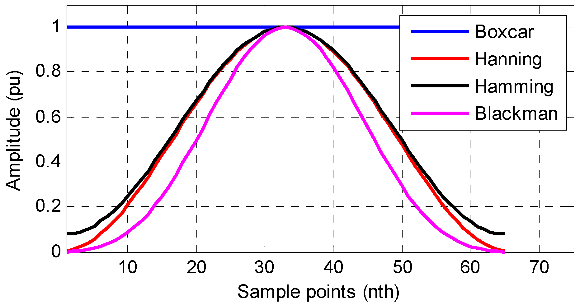
One of the popular windows is the cosine-class window, which can be expressed as:

$$w\left(n\right)=[{\displaystyle \sum }_{m=0,1,\dots }^{M}a\left(m\right)(-1{)}^{m}cos(\frac{2m\pi n}{N-1})]R_N\left(n\right)$$

(4)

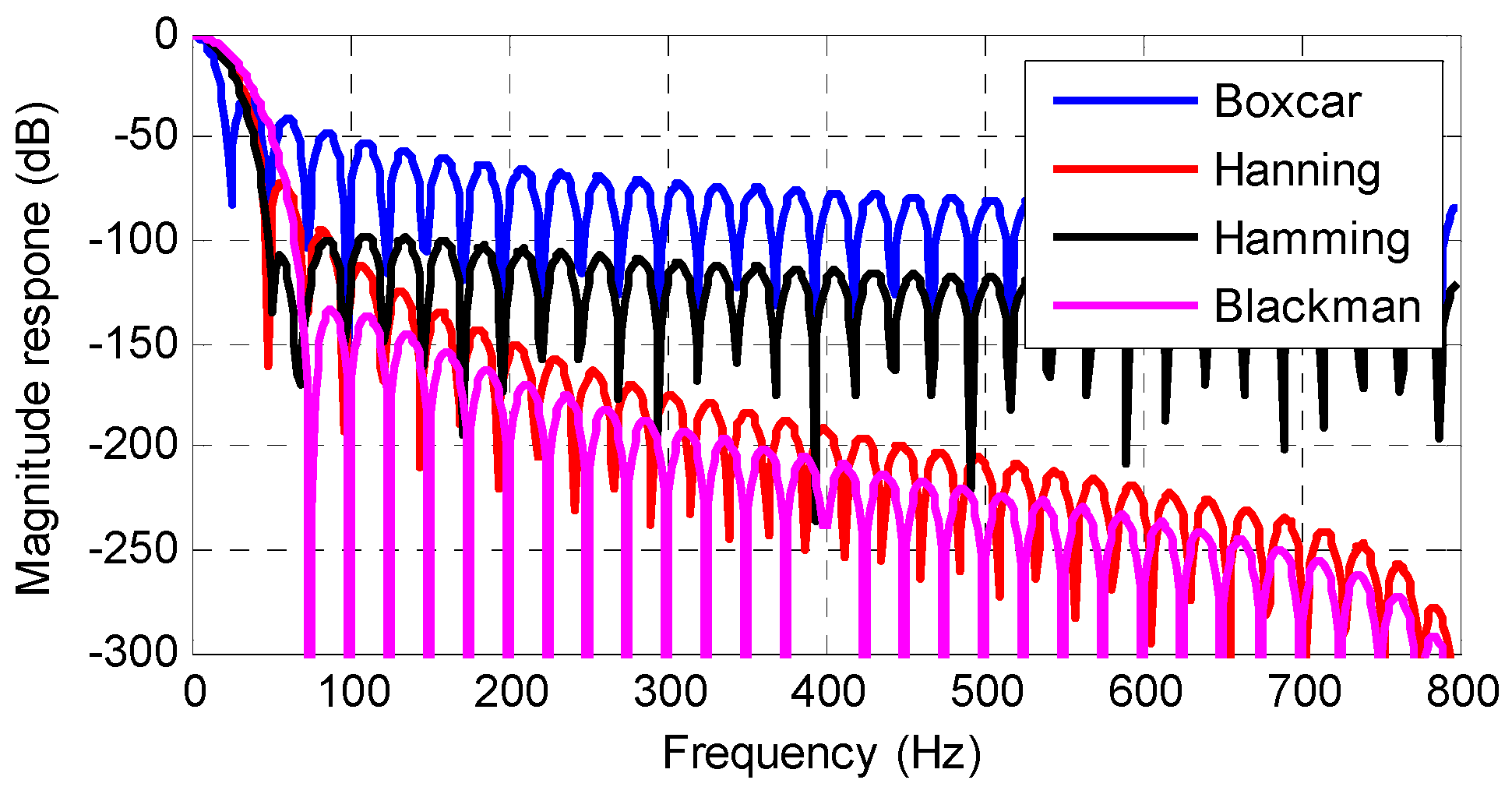
where $n=0,1,\dots ,N-1$, and $N$ is the data window length. $M$ and $a\left(m\right)$ are parameters that determine the types of the windows. For example, for $M=0, a\left(0\right)=1$, it is a boxcar window. For $M=1, a\left(0\right)=0.5, a\left(1\right)=0.5$, it is a Hanning window. For $M=1, a\left(0\right)=0.54, a\left(1\right)=0.46,$ it is a Hamming window. For $M=2, a\left(0\right)=0.42, a\left(1\right)=0.5,$ $a\left(2\right)=0.08$, it is a Blackman window.

The frequency response of the cosine-class windows can be expressed as:

$$W\left(\omega \right)=0.5[{\displaystyle \sum }_{m=0,1,\dots }^{M}a\left(m\right)W_R(\omega \pm \frac{2m\pi }{N-1})]e^{-j\frac{N-1}{2}\omega }$$

(5)

where $W_R\left(\omega \right)=sin(N\omega /2)/sin(\omega /2)$.

The waveforms of the cosine-class windows are shown in Figure 1, and the magnitude responses are shown in Figure 2. This shows that the windows have low pass characters. Thus, the windows can be applied as the LPFs to extract the quasi-dc term in Equation (3).

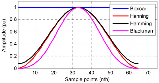
Figure 1. The magnitude responses of the cosine-class windows.

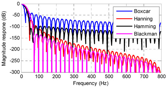
Figure 2. The magnitude responses of the cosine-class windows.

A disadvantage of the cosine-class window is that the pass band of the window is not flat, which can be seen in Figure 2. The pass band is zero if the frequency in the X-axis is zero, and it decreases quickly with the increase of frequency in the X-axis. It means that if the quasi-dc component in Equation (3) is a pure dc component, it can be extracted accurately. However, if the quasi-dc component is a low frequency component, there will be amplitude decay for the extracted component. The amplitude decay in the extracted component may induce large errors in the synchrophasor measurement. The amplitude decay can be compensated. But the compensation procedure usually needs the information of the grid frequency, which may introduce extra response delay and more computation burden in the synchrophasor measurement.

To solve this issue, flat windows with more flat pass bands are proposed in the following.

2.3. The Designed Flat Window (FW)

The FW is designed based on the LS approach. Note that after the Park’s transformation, the FFPS has been transformed into a quasi-dc component as shown in Equation (3). The quasi-dc component can be expressed as:

$$a_1\left(n\right)e^{j\Delta {\theta }_1\left(n\right)}=p_0^{\left(0\right)}+p_0^{\left(1\right)}n{T}_s+\cdots +p_0^{\left(K_0\right)}{(n{T}_s)}^{K_0}$$

(6)

where $p_0^{\left(k\right)}$ is the kth order Taylor polynomial of the quasi-dc term. $K_0$ is order of the Taylor polynomial of the quasi-dc term. Then the following equation can be obtained:

$$X=BP$$

(7)

where X is a vector of N values of $x_{dq}\left(n\right)$ in Equation (3) as $X={\left[\begin{array}{cccc}{x}_{dq}\left(n-N+1\right)& \cdots & x_{dq}\left(n-1\right)& x_{dq}\left(n\right)\end{array}\right]}^T$. B is an $N\times \left(K_0+1\right)$ matrix as $B=\left[\begin{array}{cccc}{b}_0{}^{\left(0\right)}& b_0{}^{\left(1\right)}& \cdots & b_0{}^{\left(K_0\right)}\end{array}\right]$, $b_0{}^{\left(k\right)}={\left[(\begin{array}{ccccccc}-d{)}^k& \cdots & {(-1)}^k& 0& {(1)}^k& \cdots & d^k\end{array}\right]}^T$, $d=\left(N-1\right)/2.$ P is a vector of the Taylor polynomial as $P={\left[\begin{array}{cccc}{p}_0{}^{\left(0\right)}& p_0{}^{\left(1\right)}& \cdots & p_0{}^{\left(K_0\right)}\end{array}\right]}^T$, and T is the transpose of a vector.

Then the quasi-dc term $p_0^{\left(0\right)}$ can be calculated as:

$$p_0^{\left(0\right)}=C\times X$$

(8)

where C is the coefficients of the first line of $B^{†}$, $B^{†}$ is pseudo inverse matrix of $B$ in the LS sense, and

$$B^{†}={(B^{H}B)}^{†}{B}^H$$

(9)

where $B^H$ is the conjugate transpose of $B$. Equation (8) can be expressed as:

$$p_0^{\left(0\right)}=C\times X={\displaystyle \sum }_{n=0}^{N-1}C\left(n\right)X\left(n\right)={\displaystyle \sum }_{n=0}^{N-1}h\left(N-1-n\right)X\left(n\right)$$

(10)

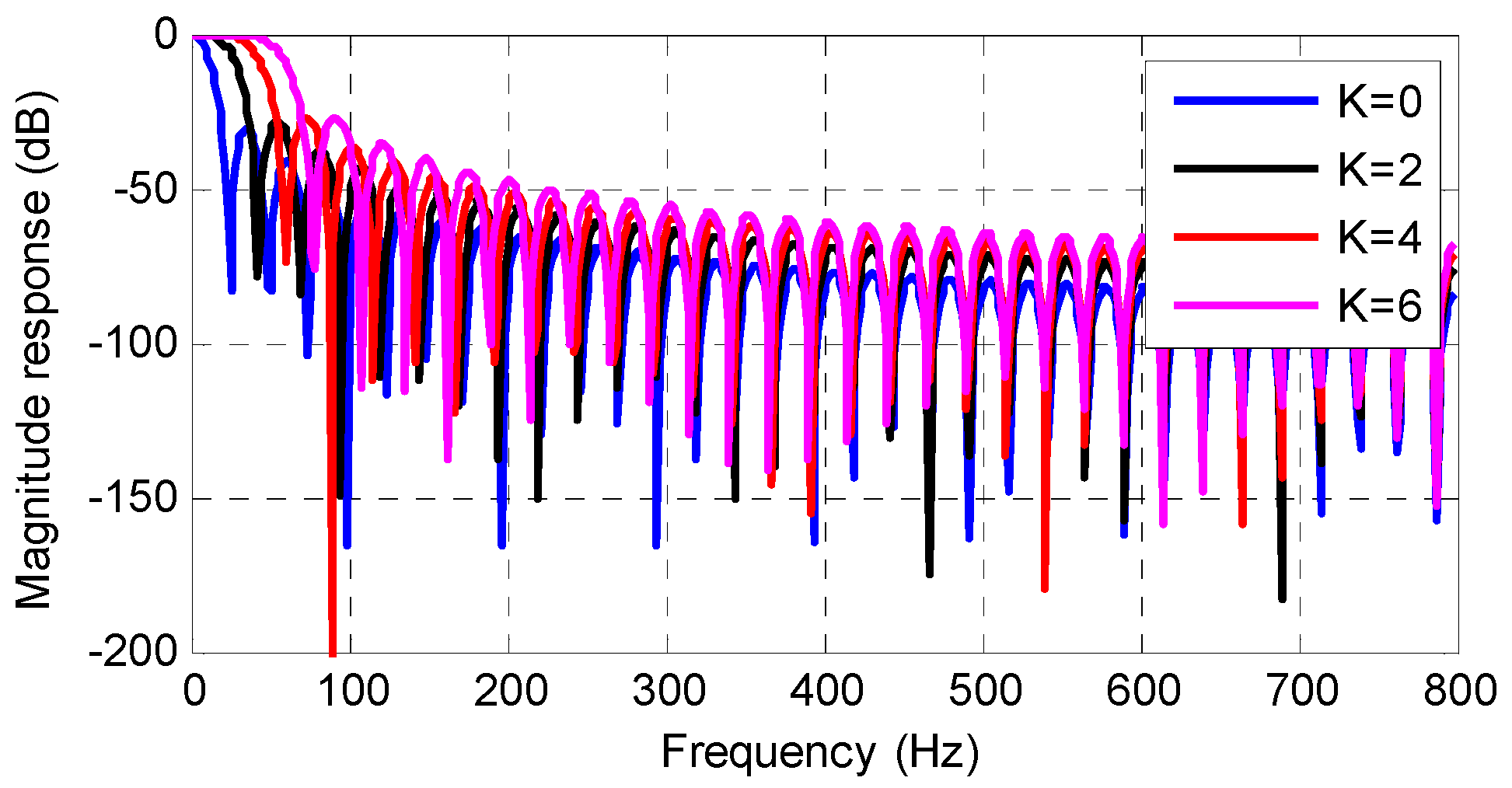
where $h\left(n\right)=C\left(N-1-n\right)$. Equation (10) can be considered as an FIR filtering process with the impulse response of $h\left(n\right)$. Different values of $K_0$ in Equation (7) result in different $h\left(n\right)$. It can be validated that $h\left(n\right)$ has flat pass band in the frequency domain, thus it is named as flat window (FW) in this paper. Figure 3 shows the waveforms of FWs with $K_0=0,1,\dots ,7$. Figure 3 shows that the odd orders of $K_0$ hardly affect the waveform of FW. Thus, the coefficients and columns corresponding to the odd polynomial orders in $P$ and $B$ can be omitted for simplification.

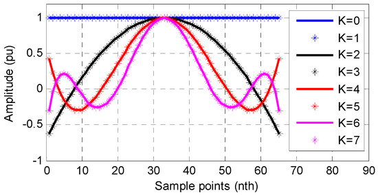
Figure 3. The waveforms of the FWs.

The corresponding frequency response for the even orders of $K_0$ are shown in Figure 4. Figure 4 shows that the FW has low pass character, and the bandwidth increases with the increase of $K_0$. The larger value of $K_0$ is, the more flat the pass band is, and vice versa. Moreover, a comparison between Figure 2 and Figure 4 shows that the designed FW has a more flat pass band than the commonly used cosine-class windows.

Figure 4. The magnitude responses of the flat windows (FWs).

Equations (6) to (10) provide a method to design the FW. The key part in the designing process is the construction of the coefficient matrix B. There are two parameters in B, namely $N$ and $K_0$. The value of $N$ affects the length of the FW, and the value of $K_0$ affects the waveform and frequency response of the FW. With the increase of $K_0$, the FW has a more flat but wider pass band, corresponding to higher measurement accuracy and longer data window length (or response time). The experiment results show that $K_0=2$ is a good choice for considering both the response time and measurement accuracy for PSMAs.

2.4. The Enhanced Flat Window (EFW)

To filter the disturbances in Equation (3), the FW should have large magnitude decay around the integer multiples of the nominal frequency. However, a detailed analysis of Figure 4 shows that the FW may not have large magnitude decay around the integer multiples of the fundamental frequency, especially in the low-frequency range. For example, the FW with $K_0=2$ has large magnitude decay around 42 Hz, 70 Hz and 95 Hz in Figure 4, while it has relatively smaller decay around 50 Hz and 100 Hz. It means that the FW has a bad filtering capability for the disturbances in Equation (3). The main reason is that in the designing process, only the quasi-dc term is considered in the LS approach in Equation (7).

The problem can be solved by considering the disturbances in the LS approach. The component in the disturbance term in Equation (3) can be expressed as:

$$\begin{array}{l}{a}_h\left(n\right)e^{j\left[{\theta }_h\left(n\right)-{\theta }_P\left(n\right)\right]}\\ =\{a_m\left(n\right)e^{j\left[\left(m+1\right)\Delta \omega n{T}_s+{\varphi }_{m+1}\left(n\right)\right]}\}{e}^{jm{\omega }_{0}n{T}_s}\\ =[p_m^{\left(0\right)}+p_m^{\left(1\right)}n{T}_s+\dots +p_m^{K_m}\left(n{T}_s{)}^{K_m}\right]e^{jm{\omega }_{0}n{T}_s}\end{array}$$

(11)

where $m=h-1$, $m=\pm 1,\pm 2,\dots ,\pm \frac{N_0}{2}-1,-\frac{N_0}{2}$, and $N_0$ is the sample points in one nominal cycle. $p_m^{\left(k\right)}$ is the kth order Taylor polynomial of the component at around $m{\omega }_0$, $K_m$ is the Taylor polynomial order of the component at around $m{\omega }_0$. If the components at $m{\omega }_0$ are considered in the LS approach, the vector $P$ and the matrix $B$ in Equation (7) should be changed into:

$$P={[\begin{array}{cc}{P}_0& P_m\end{array}]}^T,B=[\begin{array}{cc}{B}_0& B_m\end{array}]$$

(12)

where $P_0=[\begin{array}{cc}{p}_0^{\left(0\right)}& p_0^{\left(2\right)}\end{array}]$, $P_m=[\begin{array}{cccc}{p}_m^{\left(0\right)}& p_m^{\left(1\right)}& \cdots & p_m^{\left(K_m\right)}\end{array}]$, $B_0=[\begin{array}{cc}{b}_0^{\left(0\right)}& b_0^{\left(2\right)}\end{array}]$, $B_m=[\begin{array}{cccc}{b}_m^{\left(0\right)}& b_m^{\left(1\right)}& \cdots & b_m^{\left(K_m\right)}\end{array}]$, $b_m{}^{\left(k\right)}={[\begin{array}{ccccc}{(-d)}^k{e}^{-jmd{\omega }_0}& \cdots & 0^k& \cdots & d^k{e}^{jmd{\omega }_0}\end{array}]}^T$.

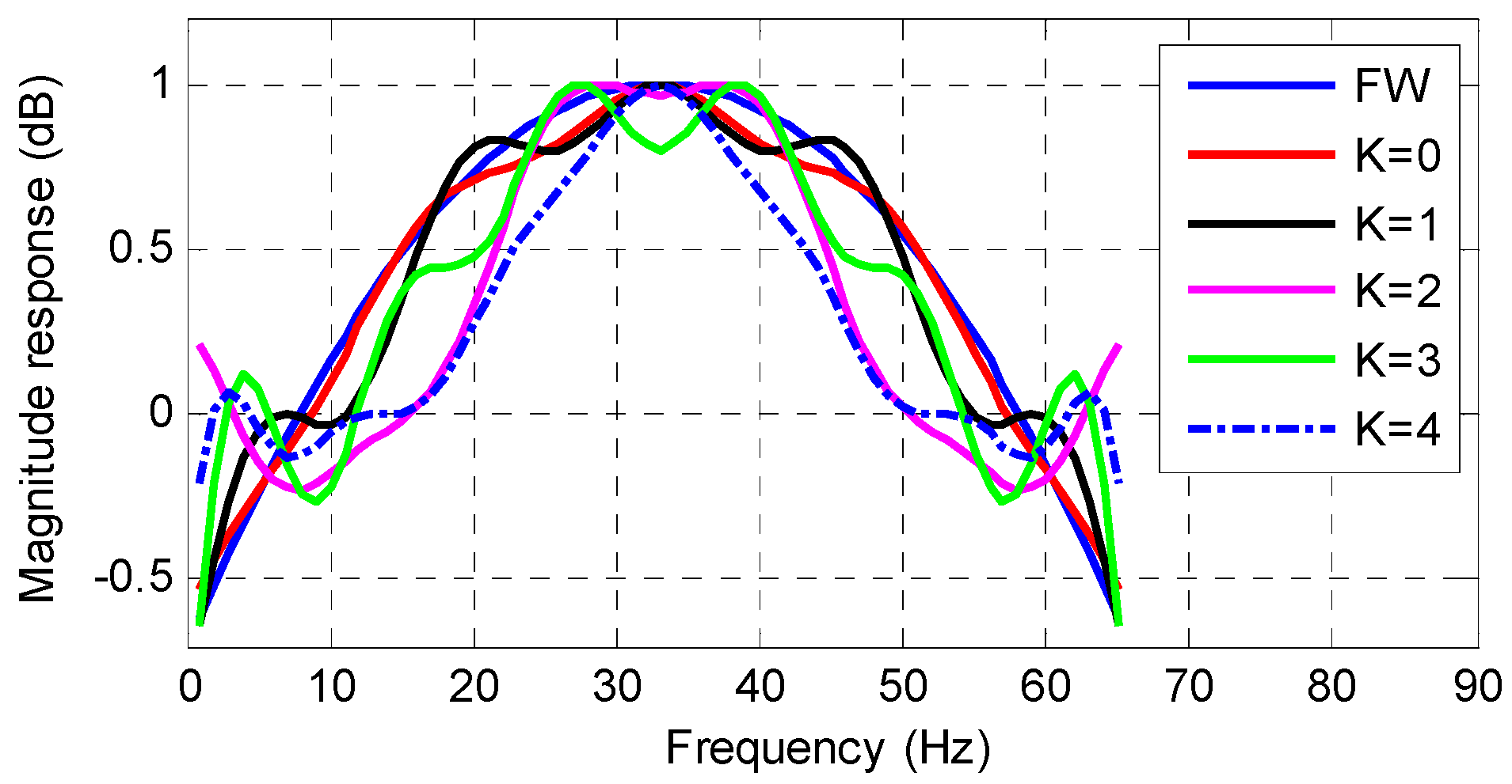
It can be validated that the obtained windows based on Equation (12) have large magnitude decay at $m{\omega }_0$. Take $m=\pm 2$ for example, the windows obtained based on Equation (12) are shown in Figure 5. The frequency responses of the obtained windows are shown in Figure 6. Note the matrix $B$ in Equation (12) is a complex matrix. However, with the consideration of $m=\pm 2$, the complex values in $B$ are conjugate pairs. Thus, the windows obtained still have real coefficients. In Figure 5 and Figure 6, the FW without the consideration of component at around $\pm 2{\omega }_0$ is also shown for a comparison.

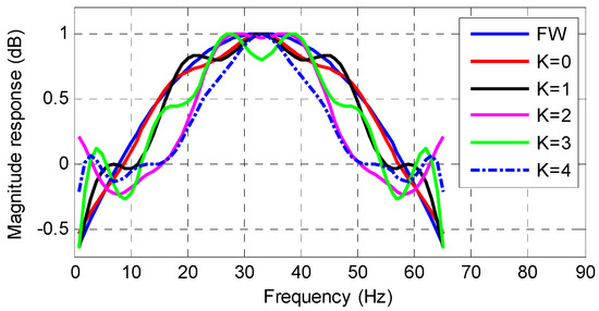
Figure 5. The waveforms of windows with the consideration of the disturbance components at $\pm 2{\omega }_0$.

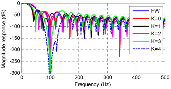
Figure 6. The magnitude responses of the windows with the consideration of the disturbance components at $\pm 2{\omega }_0$.

Figure 5 and Figure 6 show that if the component at $\pm 2{\omega }_0$ is considered in Equation (12), the obtained windows have large magnitude decay at $\pm 2{\omega }_0$. The larger order of Taylor polynomial is considered, the larger magnitude decay at this frequency is obtained at a cost of more implementation complexity. Therefore, an enhanced FW with the enhanced disturbance rejection capability is proposed in the following to solve the problem.

The components in the disturbance term in Equation (3) have frequencies around $m{\omega }_0$, and $m=\pm 1,\pm 2,\dots ,\pm \frac{N_0}{2}-1,-\frac{N_0}{2}$. Thus, zero order Taylor polynomial for these components are considered in the LS approach. Moreover, the fundamental frequency negative sequence (FFNS) component in the gird voltage signal has been transformed into a component at around $-2{\omega }_0$ after the Park’s transformation, which constructs the main disturbance in Equation (3). Thus, 3-order Taylor polynomial is applied for components at $\pm 2{\omega }_0$. Then, $P$ and $B$ in Equation (7) have been changed as:

$$P={\left[\begin{array}{ccc}{P}_0& P_m& P_2\end{array}\right]}^T,B=\left[\begin{array}{ccc}{B}_0& B_m& B_2\end{array}\right]$$

(13)

where $P_0=\left[\begin{array}{cc}{p}_0^{\left(0\right)}& p_0^{\left(2\right)}\end{array}\right]$, $P_m=\left[\begin{array}{cccc}{p}_1^{\left(0\right)}& p_{-1}^{\left(0\right)}& \cdots & p_{-N_0/2}^{\left(0\right)}\end{array}\right]$, $P_2=\left[\begin{array}{cccccc}{p}_2^{\left(1\right)}& p_{-2}^{\left(1\right)}& p_2^{\left(2\right)}& p_{-2}^{\left(2\right)}& p_2^{\left(3\right)}& p_{-2}^{\left(3\right)}\end{array}\right]$, $B_0=\left[\begin{array}{cc}{b}_0^{\left(0\right)} & b_0^{\left(2\right)}\end{array}\right]$, $B_m=\left[\begin{array}{cccc}{b}_1^{\left(0\right)}& b_{-1}^{\left(0\right)}& \cdots & b_{-N_0/2}^{\left(0\right)}\end{array}\right]$, $B_2=\left[\begin{array}{cccccc}{b}_2^{\left(1\right)}& b_{-2}^{\left(1\right)}& b_2^{\left(2\right)}& b_{-2}^{\left(2\right)}& b_2^{\left(3\right)}& b_{-2}^{\left(3\right)}\end{array}\right]$, $b_m{}^{\left(k\right)}={\left[\begin{array}{ccccc}{(-d)}^k{e}^{-jmd{\omega }_0}& \cdots & 0^k& \cdots & d^k{e}^{jmd{\omega }_0}\end{array}\right]}^T$.

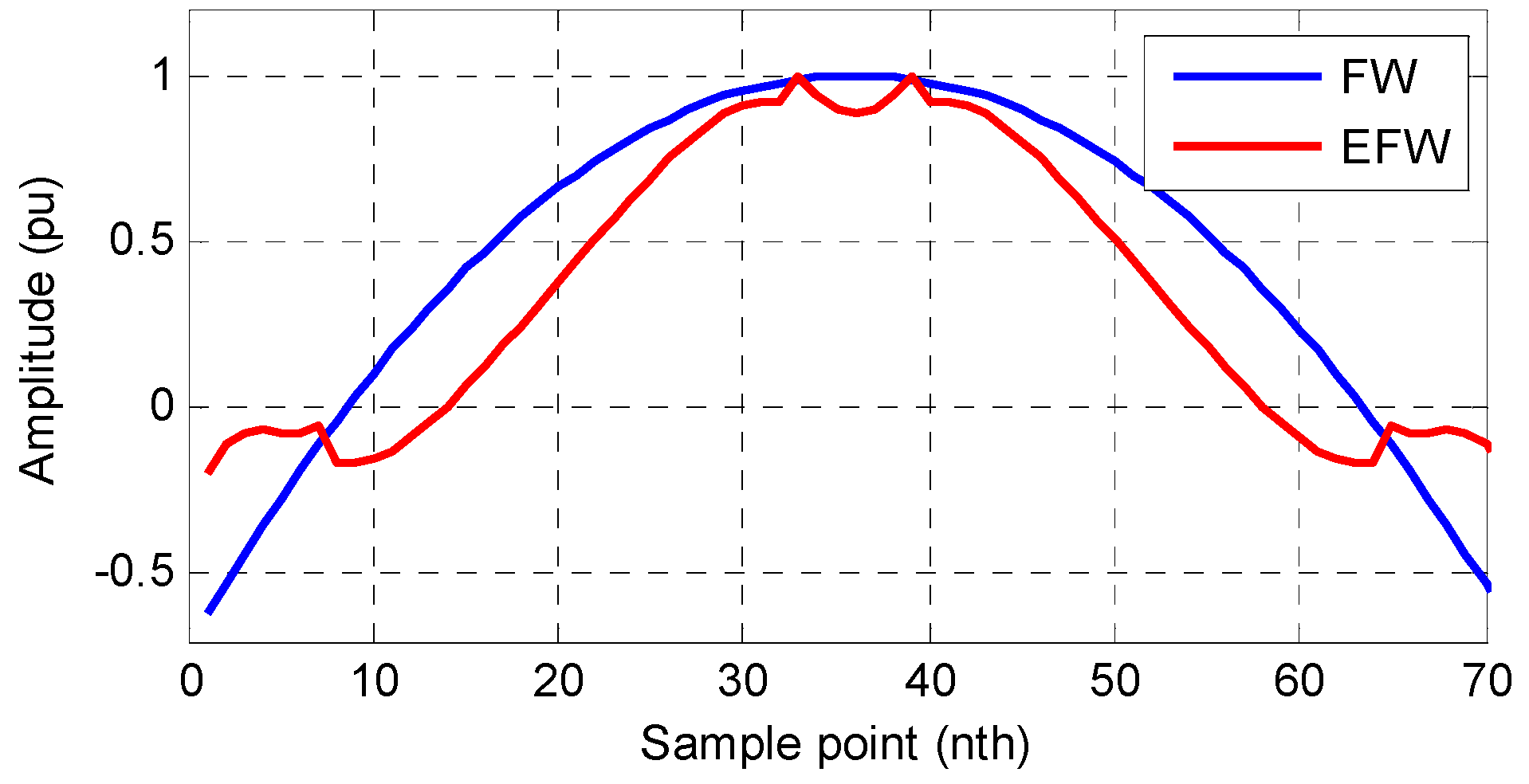
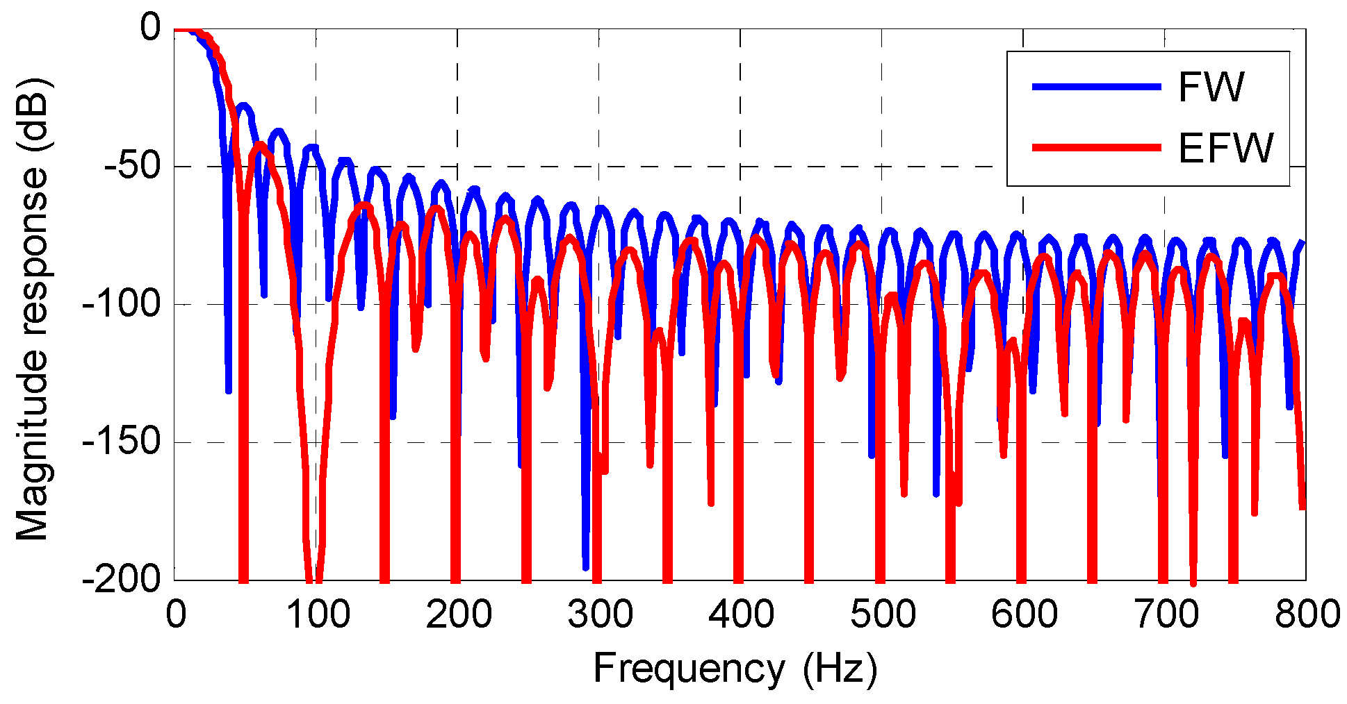
By considering the disturbance components in the LS, the obtained EFW has enhanced the disturbance rejection capability. The complex values in $B$ are conjugate pairs. Thus, the EFW still has real coefficients. The waveform of EFW is shown in Figure 7, and the frequency response of EFW is shown in Figure 8. For a comparison, the FW is also shown in Figure 7 and Figure 8. Figure 8 shows that the EFW has large magnitude decay at integer multiples of the nominal frequency, especially at $2{\omega }_0$. It means that EFW has an enhanced filtering capability for the disturbances in Equation (3). Moreover, a comparison between FW and EFW shows that the EFW has a more flat pass band and lower sidebands. Thus, the EFW is a good choice to filter the disturbance term and extract the quasi-dc term in Equation (3).

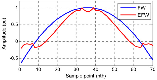
Figure 7. The waveforms of FW and enhanced flat window (EFW).

Figure 8. The magnitude responses of FW and EFW.

2.5. The Weighted Least Square (WLS)-Based Windows

Another method to design the flat window is based on the weighted least square (WLS) approach. The flat window can be designed similarly in the WLS sense based on Equations (6)–(10). The only difference is the pseudo inverse matrix in the WLS sense has been changed into:

$$B^{†}={(B^H{W}^{H}WB)}^{†}{B}^H{W}^{H}W$$

(14)

where $W$ is the weights window. The commonly used windows can be chosen as the weights window, such as the Boxcar window, the Hanning window, the Hamming window and the Blackman window.

The experiment results validate the WLS-based windows also have flat pass bands, which can be applied as the LPFs to extract the quasi-dc term in Equation (3). However, compared with the LS based windows, the WLS based windows have higher disturbance rejection capability at the cost of longer data window. Too long data window length may result in slow dynamic response under dynamics. Note that the PSMA needs a fast dynamic response, thus the LS approach based EFW is chosen for the implementation of PSMA.

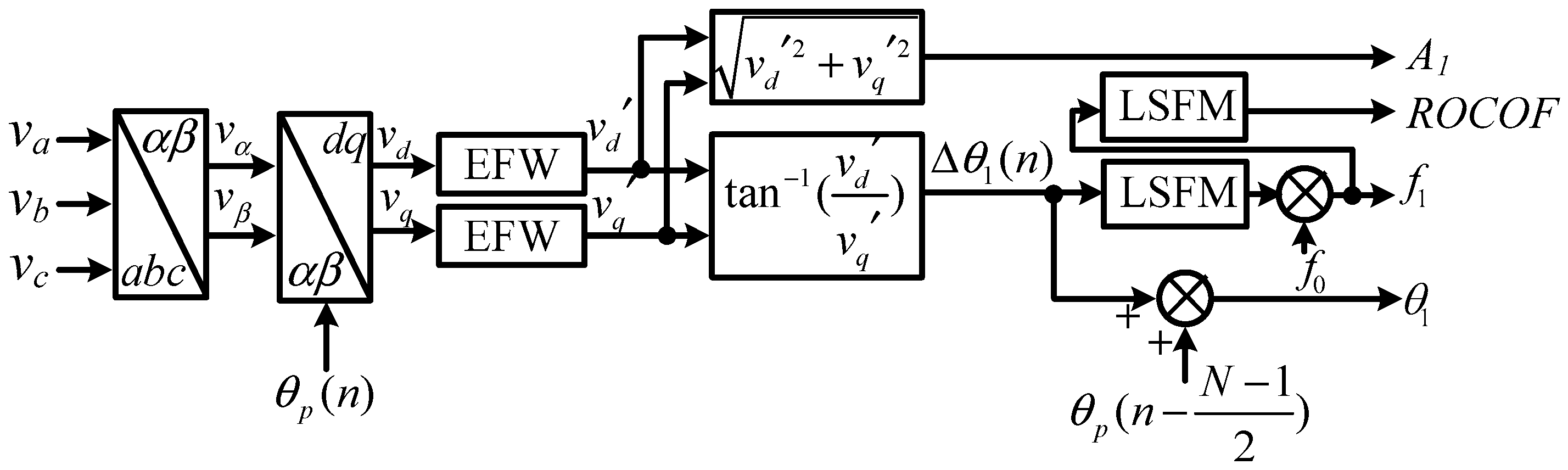
2.6. The Proposed EFW-PSMA

The basic structure of the EFW-PSMA is shown in Figure 9. Firstly, a Clarke transformation is applied to transform the grid voltage signals into the $\alpha \beta$ frame. Secondly, a Park’s transformation is applied to transform the FFPS into a quasi-dc term. Thirdly, the EFWs are adopted as the LPFs to filter the disturbances and extract the FFPS. Fourthly, the phase of the FFPS is compensated. The frequency and the rate of change of frequency (ROCOF) is calculated using the least square fitting method (LSFM) [9].

Figure 9. The structure of the enhanced flat window-based p class synchrophasor measurement algorithm (EFW-PSMA).

In Figure 9, the EFWs are adopted as the LPFs to filter the disturbance and extract the fundamental component after the Park’s transformation. The EFW has flat pass band, which ensures the measurement accuracy under dynamics and frequency deviation conditions. The EFW has enhanced filter capability for the component at integer multiples of the nominal frequency, which means EFW has an enhanced disturbance rejection capability.

The phase of the FFPS is calculated in Figure 9 as the summation of $\Delta {\theta }_1\left(n\right)$ and ${\theta }_P\left(n-\frac{N-1}{2}\right)$. The reason is as follows. The Park’s transformation in Figure 9 is equivalent to rotating the grid voltage phasor with the phase of $-{\theta }_P\left(n\right)$, and the phase of the FFPS has been transformed into $\Delta {\theta }_1\left(n\right)={\theta }_1\left(n\right)-{\theta }_P\left(n\right)$. Moreover, the estimated phase is located in the middle of the data window, thus the estimated phase is summation of the $\Delta {\theta }_1\left(n\right)$ and ${\theta }_P\left(n-\frac{N-1}{2}\right)$ as shown in Figure 9.

The frequency and ROCOF is calculated based on $\Delta {\theta }_1\left(n\right)$ using LSFM [9] in Figure 9 as follows:

$$\Delta f_1\left(n\right)=\frac{{{\displaystyle \sum }}_{m=0}^{L_f-1}{F}_m\Delta {\theta }_1\left(n-m{\phi }_{fstep}\right)}{2\pi },\begin{array}{c}\end{array}{f}_1=f_0+\Delta f_1$$

(15)

$$ROCOF\left(n\right)={\displaystyle \sum }_{m=0}^{L_{rf}-1}R{F}_m{f}_1\left(n-m{\phi }_{rfstep}\right)$$

(16)

where ${\phi }_{fstep}$ is the step between two angles, and $L_f$ is the number of angles used for a frequency estimation. ${\phi }_{rfstep}$ is the step between two frequencies, and $L_{rf}$ is the number of frequencies used for a ROCOF estimation. The values of $F_m$ and $R{F}_m$ are constant coefficients that can be calculated using the method presented in [9]. The larger values of ${\phi }_{step}$, ${\phi }_{rfstep}$, $L_f$, and $L_{rf}$ means a longer data window length for the estimation of frequency and ROCOF, corresponding to a higher measurement accuracy and slower dynamic response, and vice versa.

The EFW-PSMA has very simple implementation structure. The main computation burden is the implementation of the two EFWs in Figure 9, including 2N real multiplications and (2N-2) real additions.

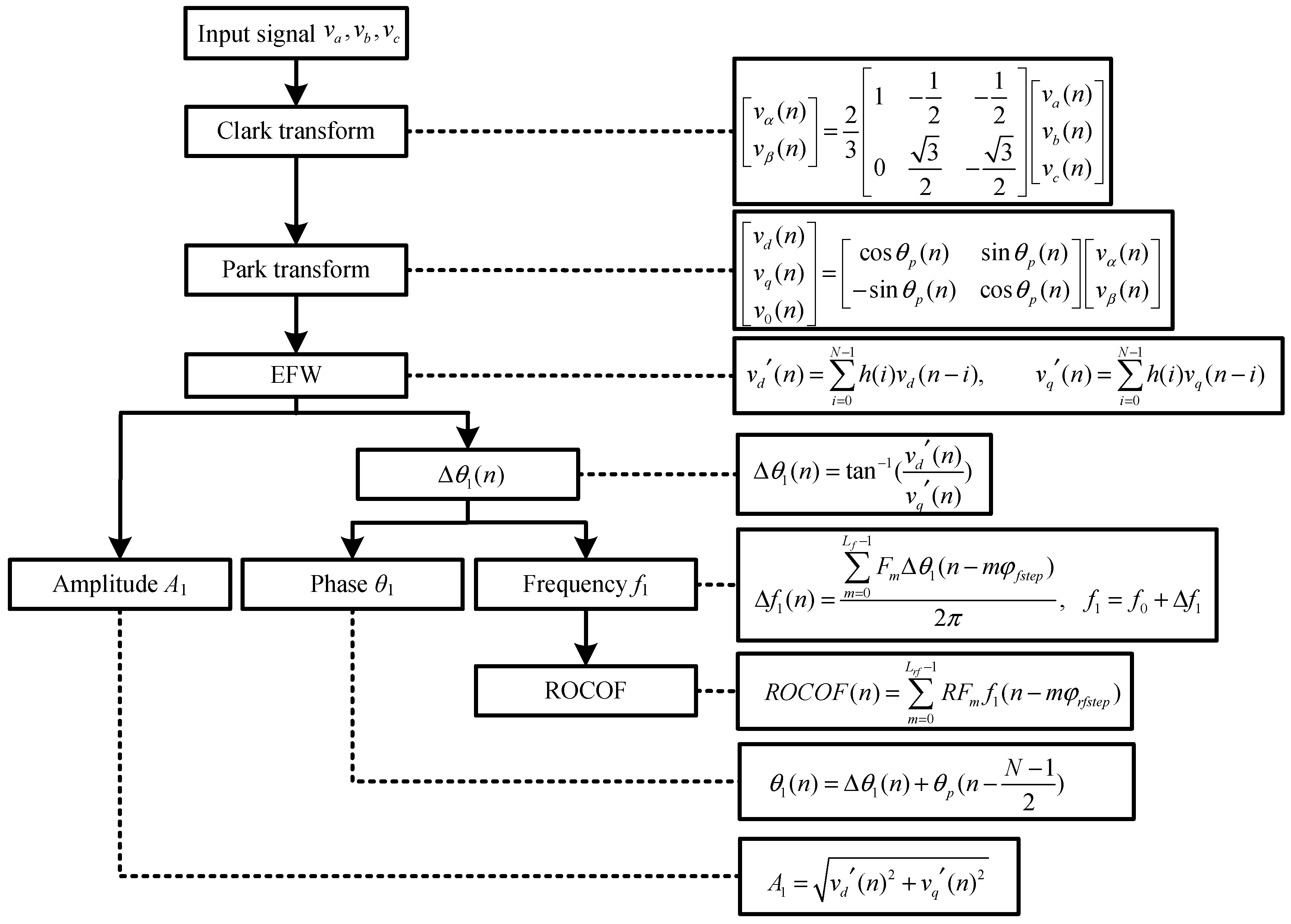
In order to explain the calculation flow of EFW-PSMA more clearly, the flowchart is shown in Figure 10. In Figure 10, X is a vector of N values of $x_{dq}\left(n\right)$ in Equation (3) as $X={\left[\begin{array}{cccc}{x}_{dq}\left(n-N+1\right)& \cdots & x_{dq}\left(n-1\right)& x_{dq}\left(n\right)\end{array}\right]}^T$. C is the coefficients of the first line of $B^{†}$, $B^{†}$ is pseudo inverse matrix of $B$ in the LS sense, B is an $N\times \left(K_0+1\right)$ matrix as $B=\left[\begin{array}{cccc}{b}_0{}^{\left(0\right)}& b_0{}^{\left(1\right)}& \cdots & b_0{}^{\left(K_0\right)}\end{array}\right]$, $b_0{}^{\left(k\right)}={\left[(\begin{array}{ccccccc}-d{)}^k& \cdots & {(-1)}^k& 0& {(1)}^k& \cdots & d^k\end{array}\right]}^T$, $d=\left(N-1\right)/2.$ The EFW can be considered as a FIR filtering process with the impulse response of $h\left(n\right)$, and the coefficients of the EFW is constant, which could be calculated once for the application.

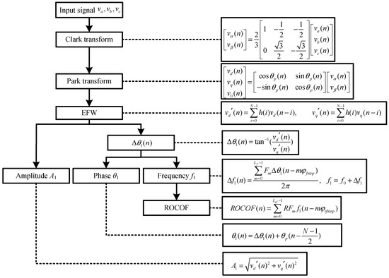
Figure 10. The implementation flowchart of the EFW-PSMA.

2.7. Formatting of Mathematical Components

To accurately set time tags for the estimated parameters, the measurement latency of the estimated parameters should be known.

The measurement latency for amplitude and phase angles is mainly caused by the implementation of the LPFs. Thus, the total measurement latency is $(\frac{N-1}{2})T_s$. Then the time tag of $t-(\frac{N-1}{2})T_s$ is used to set the time stamp for the estimated amplitude and phase angle at time instant $t$.

The measurement latency for frequency and ROCOF is mainly caused by the calculation of phasor and the LSFM in Equation (15) and Equation (16). Thus, the measurement latency for frequency and ROCOF is $(\frac{N-1}{2})T_s+\frac{{\phi }_{fstep}(L_f-1)}{2}{T}_s$ and $(\frac{N-1}{2})T_s+[\frac{{\phi }_{fstep}(L_f-1)}{2}+\frac{{\phi }_{rfstep}(L_{rf}-1)}{2}]T_s$. Therefore, the time tag of $t-[(\frac{N-1}{2})T_s+\frac{{\phi }_{fstep}(L_f-1)}{2}{T}_s]$ and $t-\{(\frac{N-1}{2})T_s+[\frac{{\phi }_{fstep}(L_f-1)}{2}+\frac{{\phi }_{rfstep}(L_{rf}-1)}{2}]T_s\}$ is used to set the time stamp for the estimated frequency at time instant $t$.

3. Performance Assessment

3.1. Response Time Assessment

The response time of the EFW-PSMA is evaluated using the step change tests.

The step changes in amplitude and phase angle can be modeled as:

$$x\left(t\right)=X_m\left[1+k_x{f}_1\left(t\right)\right]\times cos[2\pi f_{0}t+k_a{f}_1\left(t\right)]$$

(17)

where $f_1\left(t\right)$ is a unit step function, $f_0$ is the nominal frequency, $k_x$ and $k_a$ are the magnitudes of step functions in amplitude and phase angle [3].

To evaluate the performance of the EFW-PSMA under step changes, $k_x$ and $k_a$ are set to 0.1 and $\pi /18$ individually according to [3]. The parameters of EFW-PSMA are set as $N=2N_0+7$, ${\phi }_{fstep}={\phi }_{rfstep}=N_0/4$, $L_f=L_{rf}=9$. The total vector error (TVE), the frequency error (FE) and the ROCOF error (RFE) are shown in Figure 11.

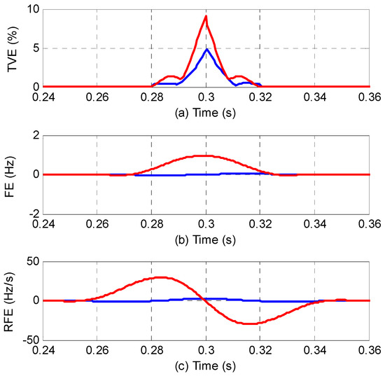
Figure 11. The dynamic response under step changes. (The blue lines are for the amplitude step test and the red lines are for the phase step test).

The results are also tabulated in Table 1 as per Standard [3] to represent the response time for TVE, FE and RFE. The limits are 1% for TVE, 0.005 Hz for FE, and 0.4 Hz/s for RFE. The response time specified in IEC/IEEE 60255-118-1 [3] is also shown in Table 1. Figure 11 and Table 1 show that the response time of EFW-PSMA satisfies well the requirements specified in IEC/IEEE 60255-118-1.

Table 1. Response time under step change tests.

	TVE Rsp.(ms)	FE Rsp.(ms)	RFE Rsp.(ms)
kx = 0.1	16	60	84
ka = π/18	30	70	100
IEC/IEEE Std.	40	90	120

3.2. Measurement Accuracy Assessment

The measurement accuracy of the EFW-PSMA is evaluated under various dynamics and distortions. The test conditions refer to [3] as follows.

Case 1(Frequency range test): The reference signal is:

$$x\left(t\right)=cos[2\pi \left(f_0+\Delta f\right)t]$$

(18)

where $f_0$ is the nominal grid frequency and $-2\le \Delta f\le 2$.

Case 2(Harmonic distortion test): The reference signal is:

$$x\left(t\right)=cos(2\pi f_{0}t)+0.01cos(2\pi h{f}_{0}t)$$

(19)

where $h$ is the order of harmonic varying from 2 to 50.

Case 3 (Frequency ramp test): The reference signal is:

$$x\left(t\right)=cos[2\pi \left(f+\Delta f+0.5R_{f}t\right)t]$$

(20)

where $\Delta f=-2$ Hz. $R_f$ is the frequency ramp rate, and $R_f=1$ Hz/s.

Case 4(Phase modulation test): The reference signal is:

$$x\left(t\right)=cos[2\pi f_{0}t+k_{a}cos(2\pi f_{m}t)]$$

(21)

where $k_a=0.1$, the modulation frequency $f_m$ varies from 0.1 to 2 Hz.

Case 5(Amplitude modulation test): The reference signal is:

$$x\left(t\right)=\left[1+k_{x}cos(2\pi f_{m}t\right)]cos(2\pi f_{0}t)$$

(22)

where $k_x=0.1$, the modulation frequency $f_m$ varies from 0.1 to 2 Hz.

Case 6(Dc-offset test): The reference signal is:

$$x\left(t\right)=0.1+cos(2\pi f_{0}t)$$

(23)

Case 7(Noise test): The reference signal is:

$$x\left(t\right)=cos(2\pi f_{0}t)+w\left(t\right)$$

(24)

where $w\left(t\right)$ is 60 dB white noise.

Case 8(Case 1 + case 2): The reference signal is:

$$x\left(t\right)=cos(2\pi ft)+0.01cos(2\pi hft)$$

(25)

where $f=f_0+\Delta f$ is the fundamental frequency, and $-2\le \Delta f\le 2$. $h$ is the order of harmonics varying from 2 to 50.

Case 9(Case 1 + Case 2 + Case 3): The reference signal is:

$$x\left(t\right)=cos(2\pi ft)+0.01cos(2\pi hft)$$

(26)

where $f=f_0+\Delta f+0.5R_{f}t$, $\Delta f=-2$ Hz and $R_f=1$ Hz/s. $h$ is the order of harmonic varying from 2 to 50.

Case 10(Case 1 + Case 2 + Case 3 + Case 4): The reference signal is:

$$x\left(t\right)=cos({\theta }_1)+0.01cos(2\pi hft)$$

(27)

where phase modulation in added in the signal model in Equation (26). ${\theta }_1=2\pi ft+k_{a}cos(2\pi f_{m}t)$, $k_a=0.1$, and the modulation frequency $f_m$ varies from 0.1 to 5 Hz.

Case 11(Case 1 + Case 2 + Case 3 + Case 4 + case 5): The reference signal is:

$$x\left(t\right)=A_{1}cos({\theta }_1)+0.01cos(2\pi hft)$$

(28)

where amplitude modulation is added in the signal model in Equation (27). $A_1=1+k_{x}cos(2\pi f_{m}t)$, $k_x=0.1$, the modulation frequency $f_m$ varies from 0.1 to 5 Hz.

Case 12(Case 1 + Case 2 + Case 3 + Case 4 + case 5 + case 6): The reference signal is:

$$x\left(t\right)=0.1+A_{1}cos({\theta }_1)+0.01cos(2\pi hft)$$

(29)

where 0.1 pu dc-offset is added in the signal model in Equation (28).

Case 13(Case 1 + Case 2 + Case 3 + Case 4 + case 5 + case 6 + case 7): The reference signal is:

$$x\left(t\right)=0.1+A_{1}cos({\theta }_1)+0.01cos(2\pi hft)+w\left(t\right)$$

(30)

where 60 dB white noise is added in the signal model in Equation (29).

Totally, 13 test cases are performed. Cases 1–5 are specified in the benchmark tests for PSMA in IEC/IEEE 60255-118-1. Noise and dc offset are not specified in the IEC/IEEE benchmark tests, yet they are unavoidable in practice. Thus, dc-offset and noise tests are added as Cases 6–7. Among the 13 test cases, single type of disturbance occurs in cases 1–7, and several types of disturbances occur simultaneously in cases 8–13. The maximum values of TVE, FE, RFE, magnitude error (ME) and phase error (PE) are presented in Table 2. The measurement accuracy requirements in the PMU Standard C37.118 are also shown in Table 2.

Table 2. The maximum measurement errors of EFW-PSMA.

Cases	Methods	ME (pu)	PE (degree)	FE (Hz)	RFE (Hz/s)	TVE (%)
1	Std.	N/A	N/A	5 × 10−3	0.4	1
	EFW-PSMA	1.4 × 10−5	2 × 10−6	2.7 × 10−6	2.2 × 10−5	1.4 × 10−3
2	Std.	N/A	N/A	5 × 10−3	0.4	1
	EFW-PSMA	4 × 10−14	3 × 10−13	2.5 × 10−11	8 × 10−10	3 × 10−11
3	Std.	N/A	N/A	0.01	0.4	1
	EFW-PSMA	6 × 10−5	1.5 × 10−5	3.1 × 10−3	1.7 × 10−4	6 × 10−3
4	Std.	N/A	N/A	0.06	2.3	3
	EFW-PSMA	2 × 10−5	2 × 10−5	0.05	1.5	6 × 10−3
5	Std.	N/A	N/A	0.06	2.3	3
	EFW-PSMA	6 × 10−5	1 × 10−5	1.3 × 10−5	1.5 × 10−4	6 × 10−3
6	Std.	N/A	N/A	N/A	N/A	N/A
	EFW-PSMA	1 × 10−13	3 × 10−13	2.5 × 10−11	1 × 10−9	3 × 10−12
7	Std.	N/A	N/A	N/A	N/A	N/A
	EFW-PSMA	1 × 10−3	8 × 10−4	6 × 10−3	0.24	0.11
8	Std.	N/A	N/A	5 × 10−3	0.4	1
	EFW-PSMA	1 × 10−3	1 × 10−3	2 × 10−3	0.04	0.11
9	Std.	N/A	N/A	0.01	0.4	1
	EFW-PSMA	3 × 10−3	1.3 × 10−3	5 × 10−3	0.012	0.22
10	Std.	N/A	N/A	0.06	2.3	3
	EFW-PSMA	4 × 10−3	2 × 10−3	0.05	1.5	0.29
11	Std.	N/A	N/A	0.06	2.3	3
	EFW-PSMA	4 × 10−3	2 × 10−3	0.05	1.5	0.35
12	Std.	N/A	N/A	0.06	2.3	3
	EFW-PSMA	4 × 10−3	2 × 10−3	0.05	1.5	0.29
13	Std.	N/A	N/A	0.06	2.3	3
	EFW-PSMA	4 × 10−3	2 × 10−3	0.05	1.7	0.32

Table 2 shows that under all the test conditions, the measurement errors of EFW-PSMA are well below the errors specified in IEC/IEEE 60255-118-1. The maximum TVE is 0.3% under the most stressed conditions that all the disturbances occurs simultaneously.

3.3. Measurement Performance Compared with the State-of-the-Art Techniques

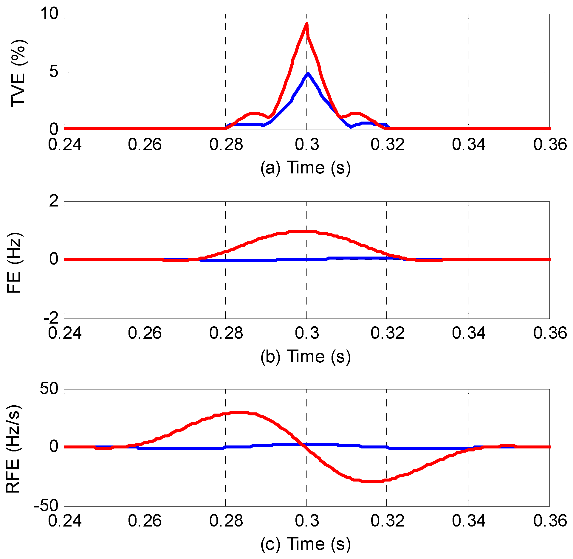
In order to show that the EFW-PSMA has better accuracy and faster response speed under the complex condition which several disturbances occur simultaneously, the EFW-PSMA is compared with the AM method [25] and the LS method [27] because the data windows of these three methods are all two cycles. The test signal is:

$$x\left(t\right)=\{\begin{array}{cc}cos2\pi f_{1}t\hfill & 0<t<0.3\\ cos(2\pi f_{1}t)+0.01cos(2\pi 2f_{1}t)\hfill & 0.3<t<0.6\\ \left[1+0.1cos(2\pi 2t\right)]\left[cos(2\pi f_{1}t\right)+0.01cos(2\pi 2f_{1}t)]\hfill & 0.6<t\end{array}$$

(31)

where $f_1=f_0+\Delta f$, $\Delta f=2$.

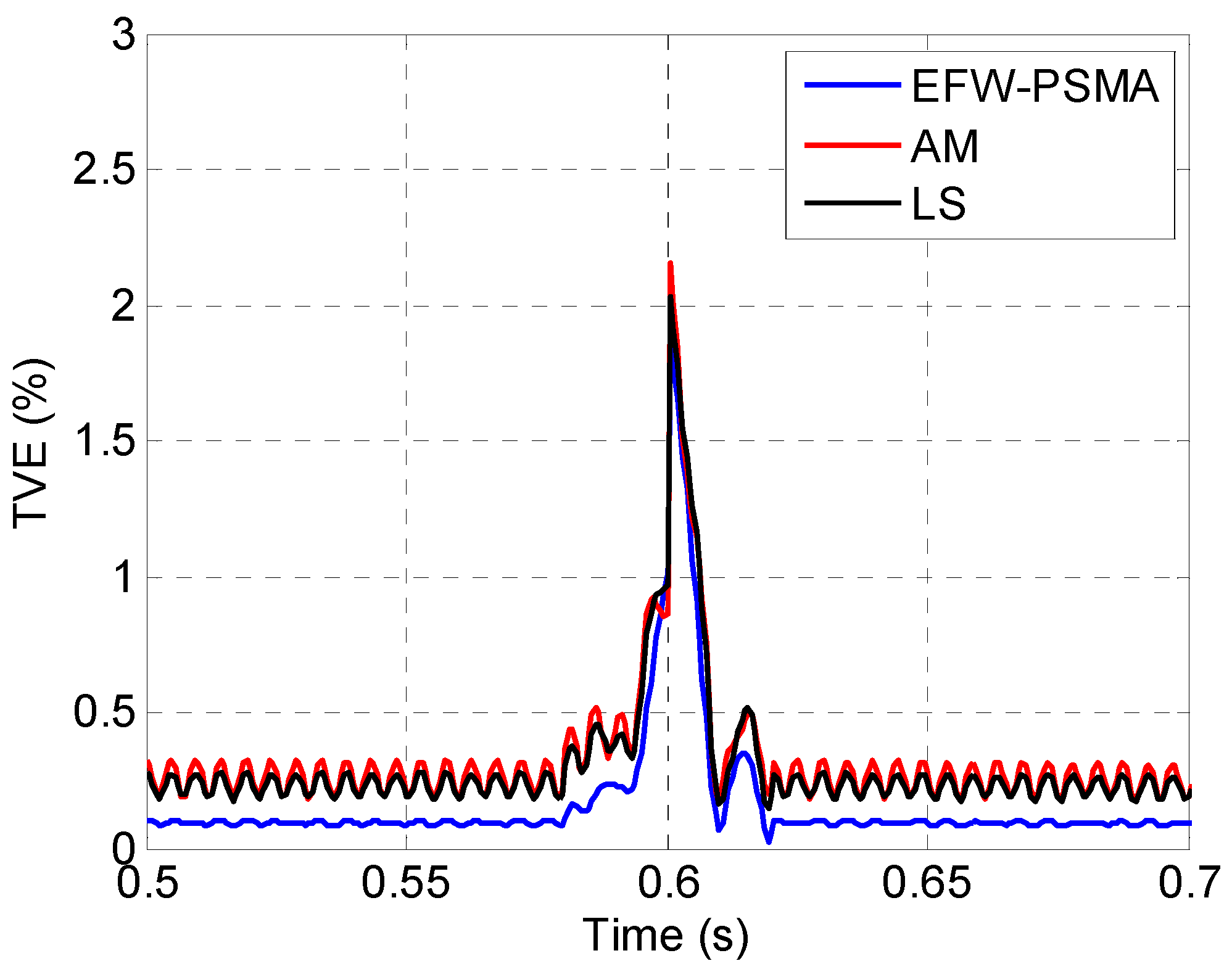
Initially, the grid voltage signal is a sinusoidal with a frequency deviation of 2 Hz, then 1% 2nd harmonic distortion is added into the signal at t = 0.3 s, next, 10% amplitude modulation is added into the signal at 0.6 s.

The TVEs of the three methods are shown in Figure 12. To give a further comparison, the zoomed in view of the period of 0.2 s to 0.4 s is shown in Figure 13, and the zoomed in view of the period of 0.5 s to 0.7 s is shown in Figure 14.

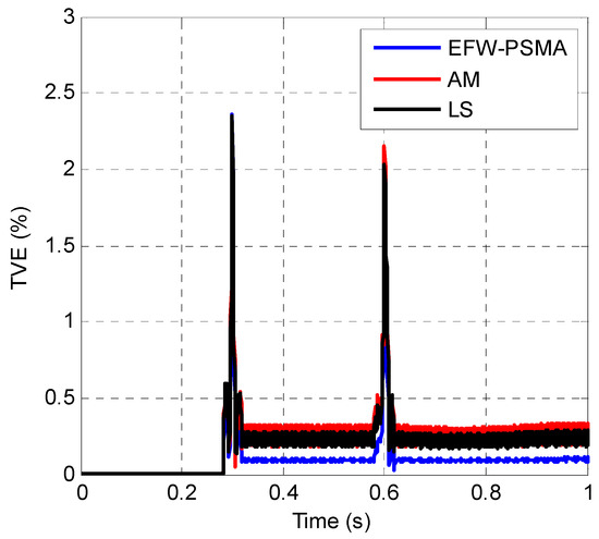
Figure 12. The TVEs of the EFW-PSMA, AM method and LS method.

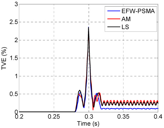
Figure 13. The zoomed in views of the period of 0.2 s to 0.4 s.

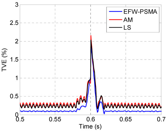
Figure 14. The zoomed in views of the period of 0.5 s to 0.7 s.

Figure 12 clearly shows that the three methods have similar performance when there is no interference, but the performance of EFW-PSMA is significantly better than the other two methods when there are multiple interferences simultaneously. Figure 13 and Figure 14 show that the three methods have similar response speeds when interference occurs because that the data windows of these three methods are all two cycles.

4. Conclusions

In this paper, a flat window with an enhanced disturbance rejection capability named EFW is designed using the least square approach. The EFWs are adopted as the LPFs in the EFW-PSMA structure to extract the fundamental component. The frequency and ROCOF are estimated based on the LS approach. The main computation burden of the EFW-PSMA includes 2N real multiplications and 2N-2 real additions. Theoretical analysis and simulation results verify the superiority of the method, especially under stressed grid conditions, where several types of disturbances occur simultaneously. Under the conditions that disturbances specified in the IEC/IEEE standard occur, the estimation errors of the EFW-PSMA are better than the standard. Under the severest condition, that is, whereby all disturbances occur simultaneously, the maximum TVE is 0.3%. In addition, EFW-PSMA is compared with the AM method and the LS method, and the result shows that the EFW-PSMA has superior measurement performance than the other two methods. This means that the EFW-PSMA can be applied to P class PMUs to measure synchrophasors quickly and accurately in order to ensure that the protection can operate correctly, which is very important for the stable operation of the power system.

References

- Castello, P.; Liu, J.; Muscas, C.; Pegoraro, P.A.; Ponci, F.; Monti, A. A Fast and Accurate PMU Algorithm for P + M Class Measurement of Synchrophasor and Frequency. IEEE Trans. Instrum. Meas. 2014, 63, 2837–2845. [Google Scholar] [CrossRef]
- Barchi, G.; Macii, D.; Belega, D.; Petri, D. Performance of Synchrophasor Estimators in Transient Conditions: A Comparative Analysis. IEEE Trans. Instrum. Meas. 2013, 62, 2410–2418. [Google Scholar] [CrossRef]
- IEC/IEEE 60255-118-1:2018—IEEE/IEC International Standard—Measuring Relays and Protection Equipment—Part 118-1: Synchrophasor for Power Systems—Measurements; IEEE: Piscataway, NJ, USA, 2018; Volume 19, pp. 1–78.
- Belega, D.; Petri, D. Accuracy Analysis of the Multicycle Synchrophasor Estimator Provided by the Interpolated DFT Algorithm. IEEE Trans. Instrum. Meas. 2013, 62, 942–953. [Google Scholar] [CrossRef]
- Romano, P.; Paolone, M. Enhanced Interpolated-DFT for Synchrophasor Estimation in FPGAs: Theory, Implementation, and Validation of a PMU Prototype. IEEE Trans. Instrum. Meas. 2014, 63, 2824–2836. [Google Scholar] [CrossRef]
- Kamwa, I.; Samantaray, S.R.; Joos, G. Wide Frequency Range Adaptive Phasor and Frequency PMU Algorithms. IEEE Trans. Smart Grid 2014, 5, 569–579. [Google Scholar] [CrossRef]
- Kamwa, I.; Pradhan, A.K.; Joos, G. Adaptive Phasor and Frequency-Tracking Schemes for Wide-Area Protection and Control. IEEE Trans. Power Deliv. 2011, 26, 744–753. [Google Scholar] [CrossRef]
- Roscoe, A.J.; Abdulhadi, I.F.; Burt, G.M. P and M Class Phasor Measurement Unit Algorithms Using Adaptive Cascaded Filters. IEEE Trans. Power Deliv. 2013, 28, 1447–1459. [Google Scholar] [CrossRef]
- Zhan, L.; Liu, Y.; Liu, Y. A Clarke Transformation-Based DFT Phasor and Frequency Algorithm for Wide Frequency Range. IEEE Trans. Smart Grid 2018, 9, 67–77. [Google Scholar] [CrossRef]
- Mai, R.K.; He, Z.Y.; Fu, L.; Kirby, B.; Bo, Z.Q. A Dynamic Synchrophasor Estimation Algorithm for Online Application. IEEE Trans. Power Deliv. 2010, 25, 570–578. [Google Scholar] [CrossRef]
- Platas-Garza, M.A.; Platas-Garza, J.; de la OSerna, J.A. Dynamic Phasor and Frequency Estimates Through Maximally Flat Differentiators. IEEE Trans. Instrum. Meas. 2010, 59, 1803–1811. [Google Scholar] [CrossRef]
- Reza, M.S.; Ciobotaru, M.; Agelidis, V.G. A Modified Demodulation Technique for Single-Phase Grid Voltage Fundamental Parameter Estimation. IEEE Trans. Ind. Electron. 2015, 62, 3705–3713. [Google Scholar] [CrossRef]
- Chen, C.I.; Chang, G.W.; Hong, R.C.; Li, H.M. Extended Real Model of Kalman Filter for Time-Varying Harmonics Estimation. IEEE Trans. Power Deliv. 2010, 25, 17–26. [Google Scholar] [CrossRef]
- Cai, X.; Wang, C.; Kennel, R. A Fast and Precise Grid Synchronization Method Based on Fixed-Gain Filter. IEEE Trans. Ind. Electron. 2018, 65, 7119–7128. [Google Scholar] [CrossRef]
- Sadinezhad, I.; Agelidis, V.G. Real-Time Power System Phasors and Harmonics Estimation Using a New Decoupled Recursive-Least-Squares Technique for DSP Implementation. IEEE Trans. Ind. Electron. 2013, 60, 2295–2308. [Google Scholar] [CrossRef]
- Das, S.; Sidhu, T. A Simple Synchrophasor Estimation Algorithm Considering IEEE Standard C37.118.1-2011 and Protection Requirements. IEEE Trans. Instrum. Meas. 2013, 62, 2704–2715. [Google Scholar] [CrossRef]
- Ren, J.; Kezunovic, M. Real-Time Power System Frequency and Phasors Estimation Using Recursive Wavelet Transform. IEEE Trans. Power Deliv. 2011, 26, 1392–1402. [Google Scholar] [CrossRef]
- Chauhan, K.; Reddy, M.V.; Sodhi, R. A Novel Distribution-Level Phasor Estimation Algorithm Using Empirical Wavelet Transform. IEEE Trans. Ind. Electron. 2018, 65, 7984–7995. [Google Scholar] [CrossRef]
- Nguyen, C.T.; Srinivasan, K. A New Technique for Rapid Tracking of Frequency Deviations Based on Level Crossings. IEEE Trans. Power Appl. Syst. 1984, PAS-103, 2230–2236. [Google Scholar] [CrossRef]
- Banerjee, P.; Srivastava, S.C. A Subspace-Based Dynamic Phasor Estimator for Synchrophasor Application. IEEE Trans. Instrum. Meas. 2012, 61, 2436–2445. [Google Scholar] [CrossRef]
- Dash, P.K.; Panda, S.K.; Mishra, B.; Swain, D.P. Fast estimation of voltage and current phasors in power networks using an adaptive neural network. IEEE Trans. Power Syst. 1997, 12, 1494–1499. [Google Scholar] [CrossRef]
- Terzija, V.V.; Djuric, M.B.; Kovacevic, B.D. Voltage phasor and local system frequency estimation using Newton type algorithm. IEEE Trans. Power Deliv. 1994, 9, 1368–1374. [Google Scholar] [CrossRef]
- Karimi-Ghartemani, M.; Ooi, B.; Bakhshai, A. Application of Enhanced Phase-Locked Loop System to the Computation of Synchrophasors. IEEE Trans. Power Deliv. 2011, 26, 22–32. [Google Scholar] [CrossRef]
- Fu, L.; Zhang, J.; Xiong, S.; He, Z.; Mai, R. A Modified Dynamic Synchrophasor Estimation Algorithm Considering Frequency Deviation. IEEE Trans. Smart Grid 2017, 8, 640–650. [Google Scholar] [CrossRef]
- Vejdan, S.; Sanaye-Pasand, M.; Malik, O.P. Accurate Dynamic Phasor Estimation Based on the Signal Model Under Off-Nominal Frequency and Oscillations. IEEE Trans. Smart Grid 2017, 8, 708–719. [Google Scholar] [CrossRef]
- Macii, D.; Petri, D.; Zorat, A. Accuracy Analysis and Enhancement of DFT-Based Synchrophasor Estimators in Off-Nominal Conditions. IEEE Trans. Instrum. Meas. 2012, 61, 2653–2664. [Google Scholar] [CrossRef]
- De la O Serna, J.A. Dynamic Phasor Estimates for Power System Oscillations. IEEE Trans. Instrum. Meas. 2007, 56, 1648–1657. [Google Scholar] [CrossRef]
© 2019 by the authors. Licensee MDPI, Basel, Switzerland. This article is an open access article distributed under the terms and conditions of the Creative Commons Attribution (CC BY) license (http://creativecommons.org/licenses/by/4.0/).