Measurement of Connectedness and Frequency Dynamics in Global Natural Gas Markets

Abstract

We examine spillovers among the North American, European, and Asia–Pacific natural gas markets based on daily data. We use daily natural gas price indexes from 2 February 2009 to 28 February 2019 for the Henry Hub, National Balancing Point, Title Transfer Facility, and Japan Korea Marker. The results of spillover analyses indicate the total connectedness of the return and volatility series to be 22.9% and 32.8%, respectively. In other words, volatility is more highly integrated than returns. The results of the spectral analyses indicate the spillover effect of the return series can largely be explained by short-term factors, while that of the volatility series can be largely explained by long-term factors. The results of the dynamic analyses with moving window samples do not indicate that global gas market liquidity increases with the increasing spillover index. However, the results identify the spillover effect fluctuation caused by demand and supply.

1. Introduction

The natural gas market has registered an expanding trend, because the fuel transition from coal to natural gas is accelerating in both the industrial and power sectors to reduce greenhouse gas emissions and prevent air pollution, as well as stagnant nuclear power generation. According to BP Statistical Review of World Energy June 2019 [1], the total primary energy consumption in the world grew from 12.4 billion tonnes of oil equivalent (btoe) in 2011 to 13.9 btoe in 2018. Coal consumption was almost constant at 3.6 btoe, while natural gas consumption increased from 2.8 btoe to 3.3 btoe. As a result, the composition ratio of natural gas increased from 22.4% to 23.9%, though the composition ratio of coal decreased from 30.5% to 27.2%. Besides the traditional gas-producing countries in the Middle East and Southeast Asia, others have been increasing their presence as exporting countries, such as Australia (which has been developing large-scale gas wells, including unconventional gas fields) and the United States of America (USA) (which began to export liquefied natural gas (LNG) derived from shale gas). Furthermore, the development of gas fields has been promoted even in Africa recently. Natural gas production skyrocketed from 28 million tonnes of oil equivalent (mtoe), 457 mtoe, and 120 mtoe in 2011 to 112 mtoe, 715 mtoe, and 203 mtoe in 2018, in Australia, the USA, and all of Africa, respectively. On the other hand, consumption is skyrocketing in China and the Middle East, in addition to steady consumption for the members of the Organisation for Economic Co-operation and Development (OECD). Natural gas consumption increased from 24 mtoe, 168 mtoe, and 1142 mtoe in 2011 to 243 mtoe, 476 mtoe, and 1505 mtoe in 2018 in China, all of the Middle East, and the OECD countries.

In the European market, progress in the deregulation of gas business and the decreasing trend of the proportion of long-term contracts linked to crude oil prices has been activating an inter-market arbitrage based on gas pipelines. Moreover, in the global market, the increase in the ratio of LNG to total natural gas trading volumes, the accelerated removal of the destination restriction clause from LNG sales contracts, and the decreasing trend for the percentage of long-term contracts linked to crude oil prices are activating an intercontinental arbitrage based on LNG. As the proportion of spot trading increases, the liquidity of the natural gas market also increases significantly.

According to the Japan Fair Trade Commission of the Government of Japan [2], the natural gas market has not been flexible in terms of region, volume, and price, with the supply chain being considered a special energy market. However, as the trading volume increases with the increase in the number of producing and/or consuming countries, gas market liquidity has also become higher. As a result, the market is changing to a general commodity market.

Natural gas portfolio holders require both security and flexibility in terms of demand and supply because they have to invest heavily and trade globally. Therefore, they need to monitor the relationship between international natural gas markets in terms of revenue and risk management. As such, we adopt the spillover index developed by Diebold and Yilmaz [3] to measure return and volatility spillovers between natural gas price indexes in Europe, North America, and Asia Pacific.

Our expectations for measuring spillover effects between markets are twofold. First, we can easily grasp the potential of a portfolio with a single index obtained by analyzing the relationship of return and volatility between securities that make up that portfolio. We can also overview the potential downside risk of the portfolio without strictly measuring the value at risk and the expected shortfall by a Monte Carlo simulation. Second, we can respond to risks early by using the index as a predictive risk indicator. If we monitor the market that is the source of the spillover, investors can smoothly rebalance their portfolios.

We must test the stationarity of variables because Diebold and Yilmaz [3] develop the spillover index based on the vector moving average (VMA) representation of the vector autoregression (VAR) model. However, the approach proposed by Diebold and Yilmaz [3] is not the Granger–causality test, but just the quantification of the spillover effect. In other words, this technique does not assess whether significant information to predict returns and/or volatility exists, but only estimates how the variables are mutually influential.

However, notwithstanding these limitations of the method, we can obtain not only academic findings concerning the most remarkable transformation market, that is, the natural gas and LNG markets, but also useful information for practitioners, such as regulatory authorities, exchanges, consumers, and suppliers. Further, this index is extremely informative for long-term investment, daily trading, production, and risk management in operating companies that hold such a natural gas portfolio.

In recent years, there have been increased studies on the natural gas market in the context of de-CO₂, the shale gas revolution, and increased liquidity. Kum et al. [4], Das et al. [5], and Bildirici and Bakirtas [6] examine the relationship between natural gas consumption volume and macroeconomic indicators in major developed countries, emerging national economies, and a developing country. Acaravci et al. [7] investigates the relationship between natural gas prices and stock prices in European countries. Nakajima and Hamori [8], Atil et al. [9], Perifanis et al. [10], Tiwari et al. [11], and Xia et al. [12] analyze the relationship between natural gas prices and the other energy prices in the USA. Batten et al. [13] study the relationship between Russian natural gas prices and other energy prices. These previous studies were conducted in the context of causality, spillover, and market integration between natural gas and other economic variables. Moreover, Nakajima [14] argues whether profits can be earned by statistical arbitrage between wholesale electricity futures and natural gas futures.

However, few studies have examined natural gas market integration. Olsen et al. [15], Scarcioffolo and Etienne [16], and Ren et al. [17] discuss the market integration in North America. Nick [18], Osička et al. [19], and Bastianin et al. [20] examine the European natural gas market integration. Shi et al. [21] reveals the interrelationship of LNG prices in Asia. Furthermore, there are few studies that have investigated the natural gas market integration across several regions. Neumann [22] studies the relationship between European and North American markets. Chai et al. [23] study the relationship between the Chinese and the global market. No research has examined the global natural gas market integration, with the exception of that by Silverstovs et al. [24], analyzing the cointegrated relationship between North America, Europe, and Japan based on monthly data from before the shale gas revolution. No studies analyze the spillover effects between North American, European, and Asia-Pacific natural gas markets based on daily data.

We adopt Diebold and Yilmaz’s [3] approach to examine spillovers between global natural gas price indexes based on daily data. The correlation coefficient captures only phenomena that do not include the meaning of the relationship. Although the cointegration analysis and the Granger causality test lead to long-term equilibrium and forecast performance, it is difficult to grasp the whole picture at a glance in the case of many variables to be analyzed. Diebold and Yilmaz’s [3] approach captures not only pairwise connectedness but also total connectedness. Although Diebold and Yilmaz’s [3] approach is not suitable for dynamic descriptions such as multivariate generalized autoregressive conditional heteroscedasticity (GARCH), it is possible to capture dynamic trends with moving window samples. Moreover, we spectrally decompose the Diebold and Yilmaz [3] index by Fourier transform. Baruník and Křehlík [25] utilized the same technique for the first time and later papers applied this approach to the energy market. For instance, Toyoshima and Hamori [26] measure the spillover index for global crude oil markets and decompose it into long-, medium-, and short-term factors. Ji et al. [27] examine the spillover effects between crude oil, heating oil, gasoline, and natural gas in North America and the United Kingdom.

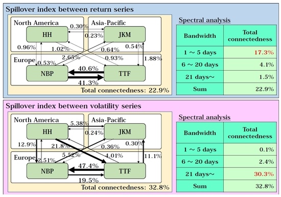
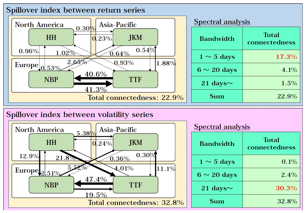
Our contribution to the literature is threefold. The contributions of this paper relate to clarifying the relationships by measuring the connectedness and its frequency dynamics in the global gas market. First, we indicate no progressing integration of the global natural gas market, although we indicate the strong spillover effect between European markets. Moreover, we indicate that the volatility is higher integrated than returns. The Diebold and Yilmaz’s [3] approach indicates that the total connectedness of return and volatility is 22.9% and 32.8%, respectively, while each total connectedness is mostly dependent on the pairwise connectedness between European natural gas price indexes. Second, our spectral analyses indicate that long-term factors contribute to volatility spillovers, while short-term factors contribute to return spillovers. We argue that arbitrage might cause short-term return spillovers and long-term memory of volatility might cause long-term volatility spillovers. Finally, our rolling analyses indicate that the above two characteristics continue. Moreover, we argue that regional climate, demand and supply, and incidents might make spillover effects larger or smaller.

The remainder of this paper is organized as follows. Section 2 describes the analyzed data, summary statistics, and preliminary basic analyses. Section 3 explains the adopted methodology. Section 4 presents the empirical results. Section 5 provides a summary of the findings and states conclusions.

2. Data and Preliminary Analyses

2.1. Data

We select natural gas price indicators for the North American, European, and Asia–Pacific markets. We use Henry Hub (HH) futures as the North American index. HH is the name of a distribution hub in Louisiana for the natural gas pipeline system in North America, referring to natural gas delivered at that hub. HH futures are listed on the New York Mercantile Exchange. We adopt National Balancing Point (NBP) and Title Transfer Facility (TTF) futures as the European index. NBP futures are futures of natural gas at a virtual trading location in the United Kingdom, being listed on the Intercontinental Exchange (ICE). This market is related to production in the North Sea gas field, which is trading with the European continent by pipelines, and consumption within the United Kingdom. TTF futures are the futures of natural gas at a virtual trading point in the Netherlands, being listed on the ICE. This market reflects the continental European market, which consists of trading by long-haul pipelines and LNG. We utilize the Japan/Korea Marker (JKM) as the Asia-Pacific index, which is associated with the short-term trading market for LNG in the Asia–Pacific region. It is provided by Platts, which assesses benchmark prices in physical energy markets. We obtain the daily data from February 2, 2009 to February 28, 2019 from Bloomberg.

Figure 1 shows the time series for these indexes. First, HH fluctuates independently from the other variables. Second, the two European indexes move together. Finally, JKM is linked to the European market over a specific period. As a result of the Great East Japan Earthquake on 11 March 2011, the amount of power generated by nuclear power plants has decreased significantly in Japan. Thus, we can assume that the Asia-Pacific LNG market was tight, and therefore the JKM was soaring. Moreover, these European indexes might have increased as a result of arbitrage trading with the Asia-Pacific LNG market. HH’s downtrend around 2012 might be caused by the expectations of increased shale gas production, while the price spike in 2014 was caused by the North American cold wave.

Figure 1. Time series plots of natural gas price. (HH = Henry Hub, NBP = National Balancing Point, TTF = Title Transfer Facility, JKM = Japan/Korea Marker).

Table 1 presents the summary statistics of the return and volatility series of each index. There are 2436 observations in each case. The JKM return series has a distribution biased to the right and the other series have distributions biased to the left, as skewness is negative only for the JKM return series. The kurtosis of all series are extremely large. In other words, all series have fat tail distributions. We can reject the hypothesis that each series is normally distributed by the Jarque-Bera statistics calculated from the skewness and kurtosis of each series.

Table 1. Summary statistics.

Statistic	Return				Volatility *
	Henry Hub (HH)	National Balancing Point (NBP)	Title Transfer Facility (TTF)	Japan/Korea Marker (JKM)	HH	NBP	TTF	JKM
Observations	2436	2436	2436	2436	2436	2436	2436	2436
Mean	0.0%	0.0%	0.0%	0.0%	2.9%	2.3%	2.0%	1.3%
Median	−0.1%	−0.1%	−0.1%	−0.0%	2.7%	2.1%	1.8%	1.0%
Maximum value	30.7%	42.9%	29.6%	15.4%	8.7%	11.2%	7.9%	10.4%
Minimum value	−16.5%	−12.3%	−12.0%	−22.6%	1.3%	0.7%	0.7%	0.3%
Standard deviation	3.2%	2.7%	2.3%	1.7%	1.1%	1.0%	0.9%	0.8%
Skewness	0.92	2.3	1.5	–0.9	1.5	1.6	1.3	3.0
Kurtosis	10.0	35.0	21.0	31.3	6.5	9.0	5.6	21.2
Jarque–Bera	5358	106,011	33,912	81,799	2182	4654	1353	37,478
(p-value)	(0)	(0)	(0)	(0)	(0)	(0)	(0)	(0)

*: calculated by the stochastic volatility (SV) model.

As described in Toyoshima and Hamori [26], let $x_t$ be a return with mean zero and variance $exp\left(h_t\right)$. The SV model can be expressed as follows:

$$x_t|h_t~N\left(0, exp\left(h_t\right)\right)$$

$$h_t|h_{t-1}, \mu , \phi , {\sigma }_{\tau } ~N\left(\mu +\phi \left(h_{t-1}-\mu \right),{\sigma }_{\tau }^2\right)$$

$$h_0|\mu , \phi , {\sigma }_{\tau } ~N\left(\mu ,{\sigma }_{\tau }^2/\left(1-{\phi }^2\right)\right)$$

where $\mu$, $\phi$, and ${\sigma }_{\tau }$ are the level of log variance, the persistence of log variance, and the volatility of log variance, respectively.

2.2. Preliminary Analyses

The condition for the VMA representation of the VAR model is that all variables are stationary. Accordingly, we test for the stationarity status of all series by the augmented Dickey–Fuller (ADF) test. Table 2 presents the results. The ADF test rejects the null hypothesis that all variables have a unit root. Therefore, we can utilize the VMA representation.

Table 2. Unit root tests.

Series	Variables	Exogenous	ADF–t Value (p-Value)
Return	Henry Hub (HH)	Constant	−54.12 (0.000)
		Constant, Trend	−54.11 (0.000)
	National Balancing Point (NBP)	Constant	−48.85 (0.000)
		Constant, Trend	−48.84 (0.000)
	Title Transfer Facility (TTF)	Constant	−47.65 (0.000)
		Constant, Trend	−47.64 (0.000)
	Japan/Korea marker (JKM)	Constant	−19.70 (0.000)
		Constant, Trend	−19.73 (0.000)
Volatility	HH	Constant	−5.13 (0.000)
		Constant, Trend	−5.31 (0.000)
	NBP	Constant	−7.18 (0.000)
		Constant, Trend	−7.26 (0.000)
	TTF	Constant	−6.29 (0.000)
		Constant, Trend	−6.37 (0.000)
	JKM	Constant	−16.60 (0.000)
		Constant, Trend	−16.85 (0.000)

We calculate the correlation coefficients over the entire period, namely from 2 February 2009 to 28 February 2019, to understand the simultaneous relationship between variables as a phenomenon. Table 3 and Table 4 present the correlation coefficients for the return and volatility series, respectively. The correlation coefficient between the NBP and TTF is the largest for both the return and volatility series. Furthermore, the correlation coefficients of the volatility series are larger than those of the return series under each combination of variables. This fact indirectly indicates the high sustainability of volatility.

Table 3. Correlation coefficient of return series.

Variables	Henry Hub (HH)	National Balancing Point (NBP)	Title Transfer Facility (TTF)	Japan/Korea Marker (JKM)
HH	1.000
NBP	0.064	1.000
TTF	0.089	0.798	1.000
JKM	0.047	0.102	0.095	1.000

Table 4. Correlation coefficient of volatility series.

Variables	Henry Hub (HH)	National Balancing Point (NBP)	Title Transfer Facility (TTF)	Japan/Korea Marker (JKM)
HH	1.000
NBP	0.397	1.000
TTF	0.465	0.940	1.000
JKM	0.223	0.402	0.465	1.000

We estimate the coefficient of the diagonal Baba, Engle, Kraft, and Kroner (BEKK) GARCH model to calculate the dynamic correlation coefficients. The BEKK model is one of several variations of multivariate GARCH models depending on the formulation of the time-varying variance–covariance matrix. The BEKK model was developed by Engle and Kroner [28], and it guarantees a positive estimated variance. Moreover, the BEKK model can dynamically calculate the correlation coefficient. When there are $k$ variables, the variance-covariance matrix $H_t$ of the BEKK model is as follows:

$$H_t=L^{\prime }L+{{\rm M}}^{\prime }{\epsilon }_{t-1}{\epsilon }_{t-1}^{\prime }{\rm M}+N^{\prime }{H}_{t-1}N$$

(1)

where ${\rm M}$ and $N$ are a $k\times k$ matrix, and $L$ is a $k\times k$ symmetric matrix.

Figure 2 provides the time series of the dynamic correlation coefficients between each pair of return series. Although the NBP and TTF have the highest correlation coefficient in Table 4, even that dynamic correlation coefficient temporarily decreases to 0. Conversely, even if a correlation coefficient over the entire period is low, the dynamic correlation coefficient may temporarily increase.

Figure 2. Dynamic correlation between each return series.

Figure 3 provides the time series of the dynamic correlation coefficients between each volatility series. We find that the correlation and inverse correlation phases are clear because volatility accumulates at a high rate. However, only the dynamic correlation coefficient between the NBP and TTF continues to be almost +1.

Figure 3. Dynamic correlation between each volatility series.

3. Methodology

3.1. Spillover Index

A correlation coefficient only represents a simultaneous phenomenon between variables. Therefore, our analysis on the relationship between variables needs to go further. We begin by calculating the index proposed by Diebold and Yilmaz [3] which can capture the spillover effect between variables.

We assume the following covariance stationary four-variable VAR ($p$):

$$x_t={\displaystyle \sum }_{l=1}^p{\Phi }_l{x}_{t-l}+{\epsilon }_t,$$

(2)

where $x_t$ is the four-dimensional vector of return or volatility, which must be a stationary series; ${\Phi }_l$ are the $4\times 4$ coefficient matrices; $p$ is the lag length based on the Schwarz information criterion; and ${\epsilon }_t$ is an independently and identically distributed sequence of four-dimensional random vectors with zero mean and covariance matrix $\mathrm{E}\left({\epsilon }_t{\epsilon }_t^{\prime }\right)=\Sigma$.

We can represent the above VAR model in the following VMA:

$$x_t={\displaystyle \sum }_{l=0}^{\infty }{A}_l{\epsilon }_{t-l}$$

(3)

where $A_l={\sum }_{l=1}^p{\Phi }_l{A}_{t-l}$, $A_0$ being a $4\times 4$ identity matrix with $A_l=0$ for $l<0$.

We define the spillover effect from the $m$th to the $l$th market up to $H$-step-ahead as the following equation by using the $H$-step-ahead forecast error variance decompositions:

$${\theta }_{lm}=\frac{{\sigma }_{mm}^{-1}{\sum }_{h=0}^{H-1}{\left(e_l^{\prime }{A}_h\Sigma e_m\right)}^2}{{\sum }_{h=0}^{H-1}{e}_l^{\prime }{A}_h\Sigma A_h^{\prime }{e}_l}$$

(4)

where ${\sigma }_{mm}$ is the standard deviation of the error term for the $m$th equation and $e_l$ is the selection vector, with one as the $l$th element and zeros otherwise.

We normalize each entry of the variance decomposition matrix by the row sum, that is, 4, as the pairwise connectedness:

$$\widetilde{{\theta }_{lm}}=\frac{{\theta }_{lm}}{{\sum }_{m=1}^4{\theta }_{lm}}=\frac{{\theta }_{lm}}{4}$$

(5)

We define the sum of pairwise connectedness as total connectedness:

$$S=\frac{{\sum }_{l=1}^4{\sum }_{m=1,l\ne m}^4\widetilde{{\theta }_{lm}}}{4}$$

(6)

The numerator is the sum of the spillover effects, excluding the spillover effects on itself. In other words, the total connectedness means the sum of the relative proportion of the portfolio’s response to a shock.

Moreover, we measure the directional spillover effects received by the $l$th market from all other markets as:

$$S_{l·}=\frac{{\sum }_{l=1,l\ne m}^4\widetilde{{\theta }_{lm}}}{4}$$

(7)

Similarly, we measure the directional spillover effects transmitted by the $l$th market to all other markets as:

$${S.}_l=\frac{{\sum }_{l=1,l\ne m}^4\widetilde{{\theta }_{ml}}}{4}$$

(8)

3.2. Spectral Analysis

Based on the Fourier transform utilized by Baruník and Křehlík [25], we spectrally decompose Diebold and Yilmaz’s [3] indexes into short-term (1 to 5 business days) factors, medium-term (6 to 20 business days) factors, and long-term (from 21 business days onward) factors.

The Fourier transform of Equation (2) is as follows:

$$f{\left(\omega \right)}_{lm}=\frac{{\sigma }_{mm}^{-1}{\left({\left(({\sum }_{h=0}^{H-1}{e}^{-i\omega h}{A}_h)\Sigma \right)}_{lm}\right)}^2}{{\left(({\sum }_{h=0}^{H-1}{e}^{-i\omega h}{A}_h)\Sigma ({\sum }_{h=0}^{H-1}{e}^{i\omega h}{A}_h){}^{\prime }\right)}_{ll}}$$

(9)

This is the spillover effect from the $m$th market to the $l$th market up to $H$-step-ahead, which is expressed by angular frequency $\omega$.

We define the weighting function, the ratio of $\omega$ component to all-frequency components concerning the spillover to the $l$th variable, as follows:

$${\Gamma }_l\left(\omega \right)=\frac{{\left(\left({\sum }_{h=0}^{H-1}{e}^{-i\omega h}{A}_h\right)\Sigma \left({\sum }_{h=0}^{H-1}{e}^{i\omega h}{A}_h\right){}^{\prime }\right)}_{ll}}{\frac{1}{2\pi }{\int }_{-\pi }^{\pi }{\left(\left({\sum }_{h=0}^{H-1}{e}^{-i\lambda h}{A}_h\right)\Sigma \left({\sum }_{h=0}^{H-1}{e}^{i\lambda h}{A}_h\right){}^{\prime }\right)}_{ll}d\lambda }$$

(10)

The spillover index from the $m$th market to the $l$th market in all bands is expressed as:

$${\left({\theta }_{\infty }\right)}_{lm}=\frac{1}{2\pi }{\int }_{-\pi }^{\pi }{\Gamma }_l\left(\omega \right)f{\left(\omega \right)}_{lm}d\omega$$

(11)

The spillover index from the $m$th market to the $l$th market in band $d$ is expressed as:

$${\left({\theta }_d\right)}_{lm}=\frac{1}{2\pi }{\int }_d{\Gamma }_l\left(\omega \right)f{\left(\omega \right)}_{lm}d\omega$$

(12)

We convert ${\left({\theta }_d\right)}_{lm}$ to the relative contribution ${\left(\widetilde{{\theta }_d}\right)}_{lm}$ as:

$${\left(\widetilde{{\theta }_d}\right)}_{lm}=\frac{{\left({\theta }_d\right)}_{lm}}{{\sum }_{l=1}^4{\left({\theta }_{\infty }\right)}_{lm}}$$

(13)

We calculate the total spillover index in the $d$ band as:

$$C_d=\frac{{\sum }_{l=1}^4{\sum }_{m=1,l\ne m}^4{\left(\widetilde{{\theta }_d}\right)}_{lm}}{{\sum }_{l=1}^4{\sum }_{m=1}^4{\left(\widetilde{{\theta }_d}\right)}_{lm}}$$

(14)

Naturally, this is consistent with Diebold and Yilmaz’s [3] spillover index.

3.3. Rolling Analysis

It is insufficient to focus on static spillover indicators, which are calculated by the Diebold and Yilmaz [3] and Baruník and Křehlík [25] for the entire period. To capture the dynamics of the spillover effects, we employ the rolling window approach as a sampling method. As shown in Figure 4, this study fixes the moving window sample size to 300 trading days and offsets the window by one business days every time we perform an analysis.

Figure 4. Illustration of moving window procedure.

4. Empirical Results

4.1. Spillover Index

The spillover analyses results of the return series are reported in Table 5. The spillover index from HH to the other variables and from the other variables to HH are 0.42% and 0.57%, respectively. HH fluctuates independently of the other variables.

Table 5. Spillover index between return series.

To	From
	Henry Hub (HH)	National Balancing Point (NBP)	Title Transfer Facility (TTF)	Japan/Korea Marker (JKM)	Others
HH	98.3	0.53	0.93	0.23	0.42
NBP	0.96	57.8	40.6	0.64	10.5
TTF	1.02	41.3	57.2	0.54	10.7
JKM	0.30	2.65	1.88	95.2	1.21
Others	0.57	11.1	10.8	0.35	22.9

The spillover indexes from NBP to TTF and from TTF to NBP are both above 40%. While the total connectedness is 22.9%, the spillover indexes from the other variables to TTF and from TTF to the other variables are 10.7% and 10.8%, respectively. Moreover, the spillover indexes from the other variables to NBP and from NBP to the other variables are 10.5% and 11.1%, respectively. TTF and NBP have a high presence as both the sources and destinations of spillover effects, because these two natural gas markets in Europe are almost integrated, although HH and JKM fluctuate relatively independently. However, only the spillover index from NBP to JKM is not at a negligible level, at 2.65%.

The spillover indexes of the volatility series are reported in Table 6. The total connectedness of the volatility series is 32.8%, while the total connectedness of the return series is 22.9%. Risks tend to be transmitted between markets rather than returns. This mutual relationship is similar to the tendency of the return series. However, the characteristic of volatility series is that the influence of HH on the other variables is larger. Additionally, we hardly observe the spillover effects from JKM to the other variables.

Table 6. Spillover index between volatility series.

To	From
	Henry Hub (HH)	National Balancing Point (NBP)	Title Transfer Facility (TTF)	Japan/Korea Marker (JKM)	Others
HH	93.3	2.51	4.01	0.24	1.69
NBP	12.9	39.3	47.4	0.36	15.2
TTF	21.8	19.5	58.4	0.30	10.4
JKM	5.38	5.52	11.1	78.0	5.49
Others	10.0	6.88	15.6	0.22	32.8

4.2. Spectral Analysis

The spectral analyses results of the return series spillover are reported in Table 7. The total connectedness from 1 to 5 business days, from 6 to 20 business day, and over 21 business days is 17.3%, 4.12%, and 1.49%, respectively. The short-term factors contribute most to the return spillover. The spillover effects of the return series are mostly explained by events within about one week. Arbitrage might contribute to these short-term spillover effects.

Table 7. Spectral analyses of spillover index between return series.

Bandwidth	To	From
		Henry Hub (HH)	National Balancing Point (NBP)	Title Transfer Facility (TTF)	Japan/Korea Marker (JKM)	Others
1 to 5 business days	HH	82.1	0.39	0.72	0.18	0.32
	NBP	0.55	47.1	32.5	0.49	8.40
	TTF	0.54	31.2	45.8	0.37	8.02
	JKM	0.14	1.17	0.84	69.6	0.54
	Others	0.31	8.18	8.53	0.26	17.3
6 to 20 business days	HH	12.0	0.10	0.15	0.04	0.07
	NBP	0.30	7.94	5.93	0.11	1.59
	TTF	0.35	7.45	8.37	0.13	1.98
	JKM	0.11	1.05	0.74	18.4	0.47
	Others	0.19	2.15	1.71	0.07	4.12
21 business days onward	HH	4.29	0.04	0.05	0.01	0.03
	NBP	0.11	2.80	2.09	0.04	0.56
	TTF	0.13	2.66	2.97	0.05	0.71
	JKM	0.05	0.43	0.30	7.17	0.20
	Others	0.07	0.78	0.61	0.02	1.49

Table 8 presents the spectral analyses results of the volatility series spillovers. The total connectedness from 1 to 5 business days, from 6 to 20 business days, and over 21 business days is 0.10%, 2.37%, and 30.3%, respectively. Contrary to the return series, the long-term factors contribute most to the volatility spillover. Most of the spillover effect of the volatility series is caused by events that occurred more than one month ago. The reason might be the long-term memory of volatility.

Table 8. Spectral analyses of spillover index between volatility series.

Bandwidth	To	From
		Henry Hub (HH)	National Balancing Point (NBP)	Title Transfer Facility (TTF)	Japan/Korea Marker (JKM)	Others
1 to 5 business days	HH	0.06	0.00	0.00	0.00	0.00
	NBP	0.03	0.50	0.17	0.00	0.05
	TTF	0.02	0.15	0.20	0.00	0.04
	JKM	0.01	0.02	0.02	22.0	0.01
	Others	0.01	0.04	0.05	0.00	0.10
6 to 20 business days	HH	2.09	0.04	0.01	0.00	0.01
	NBP	0.27	7.27	3.90	0.02	1.05
	TTF	0.20	3.63	4.10	0.02	0.96
	JKM	0.12	0.75	0.55	32.6	0.35
	Others	0.15	1.10	1.11	0.01	2.37
21 business days onward	HH	91.1	2.47	4.00	0.24	1.68
	NBP	12.7	31.6	43.3	0.33	14.1
	TTF	21.6	15.7	54.1	0.28	9.39
	JKM	5.26	4.75	10.5	23.5	5.13
	Others	9.87	5.74	14.5	0.21	30.3

4.3. Rolling Analysis

4.3.1. Total Connectedness

Figure 5 shows the total connectedness of the return series and the results of its spectral analyses. The total connectedness has not fluctuated significantly for 10 years and there is no significant change in the composition ratio of the total connectedness. The short-term factors have almost caused return spillovers.

Figure 5. Total connectedness of return series.

Figure 6 represents the total connectedness of the volatility series and the results of its spectral analyses. As with the static analysis results, the long-term factors almost caused volatility spillovers.

Figure 6. Total connectedness of volatility series.

Total connectedness spikes in February 2014, February 2018, and November 2018. We assume these spikes are caused by sudden fluctuations in each series. The price of HH spikes in February 2014 because of a great cold wave. The same phenomenon occurs every winter, although the scale is small. Additionally, the JKM, NBP, and TTF prices began to decline at around same time, because the spot market, which has been tight since the Great East Japan Earthquake, shifts and becomes loose. Therefore, the spillover index spikes.

The oversupply strengthens from January to February 2018, because of the expectation to expand USA’s LNG export capacity along with the production of crude oil and natural gas. As a result, each gas price index falls sharply. Conversely, in November, the HH increases sharply because the storage stock levels in the USA fall significantly below recent levels. These facts cause the two spikes in 2018.

4.3.2. Pairwise Connectedness

Figure 7 traces the pairwise connectedness of the return series and the results of its spectral analyses. In all combinations, the spillover effects of the return series continue to depend on short-term factors. Compared to the total connectedness, which is stable at around 30%, the pairwise connectedness between any variables is low and stable, although the pairwise connectedness from NBP to JKM and from TTF to JKM temporarily reaches around 3%. The mutual spillover effects offset each other because they are almost at the same level. However, when the Asia-Pacific spot market becomes tight or loose, the European market might be relatively stronger than the Asia-Pacific one.

Figure 7. Pairwise connectedness of return series.

Figure 8 shows the pairwise connectedness of the volatility series and the results of its spectral analyses. Under all combinations, the spillover effects of the volatility series continue to depend on long-term factors. The spillover effects from HH to NBP and from TTF to JKM are periodically strong. The HH volatility spikes caused by the cold wave in North America affect the global market. In the European market, the spillover effect from TTF to NBP is stably high. TTF might be more prone to risks than NBP, because the former is more closely linked to intra-European and international trading using pipelines and LNG.

Figure 8. Pairwise connectedness of volatility series.

5. Conclusions

We adopt the approach of Diebold and Yilmaz [3] to examine the spillover effects between global natural gas price indexes. Moreover, we employ the Fourier transform utilized by Baruník and Křehlík [25] for spectrally decomposing Diebold and Yilmaz’s [3] index.

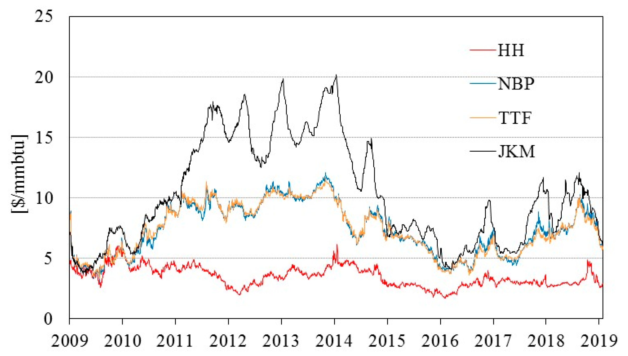
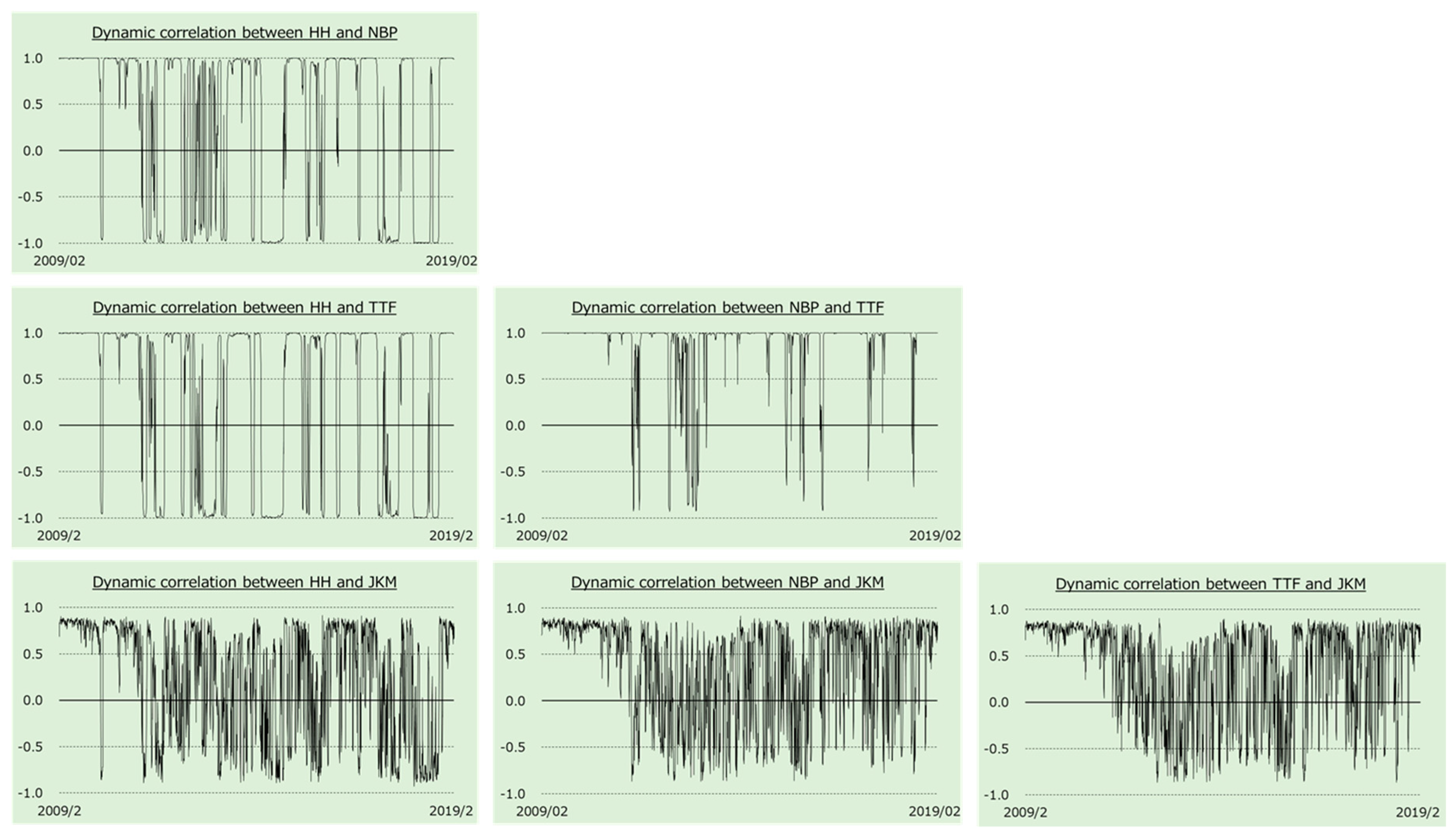
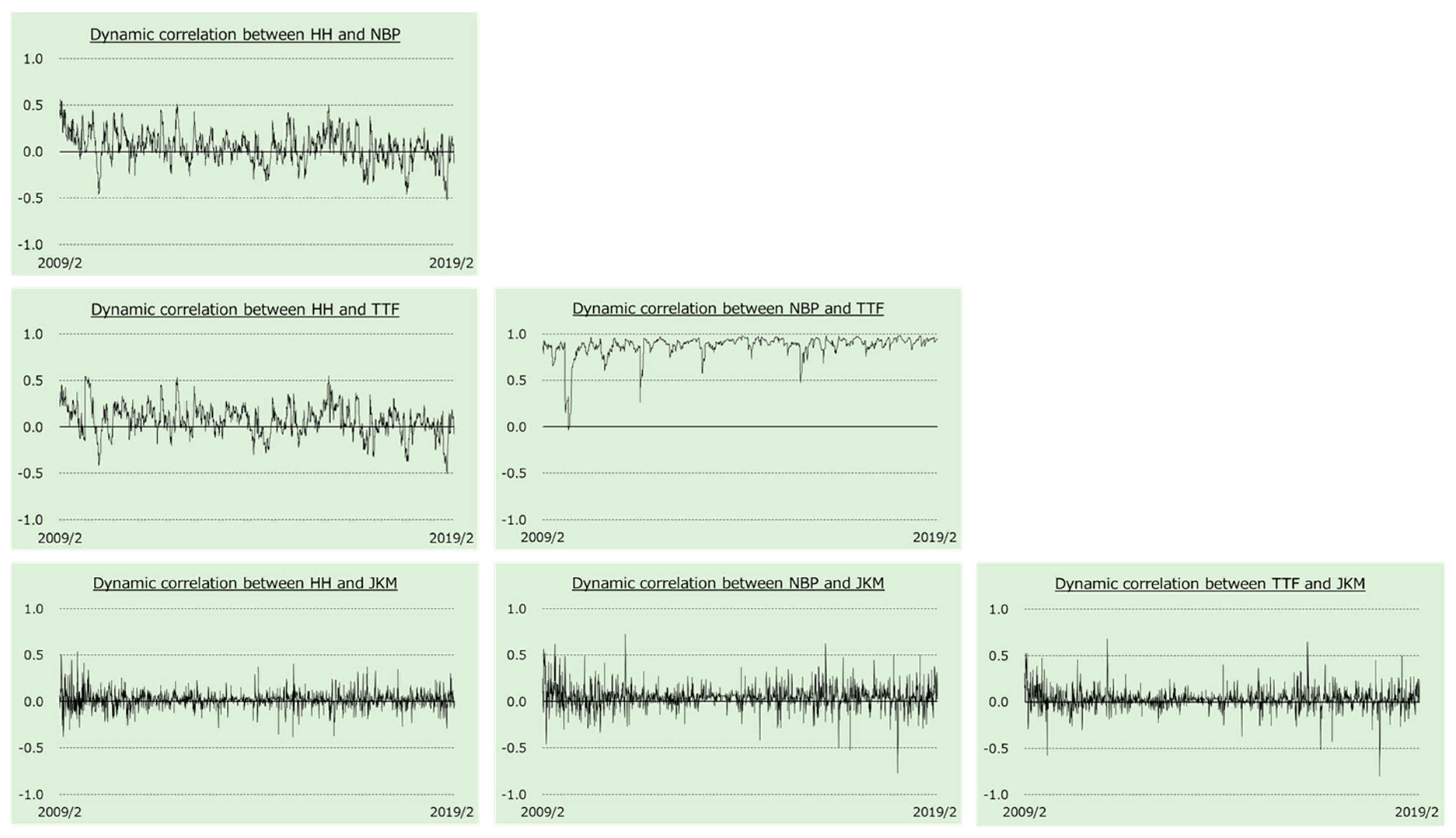
We use daily data from 2 February 2009 to 28 February 2019. We employ HH, NBP, TTF, and JKM as the North American, British, Continental European, and Asia-Pacific market price indexes, respectively.

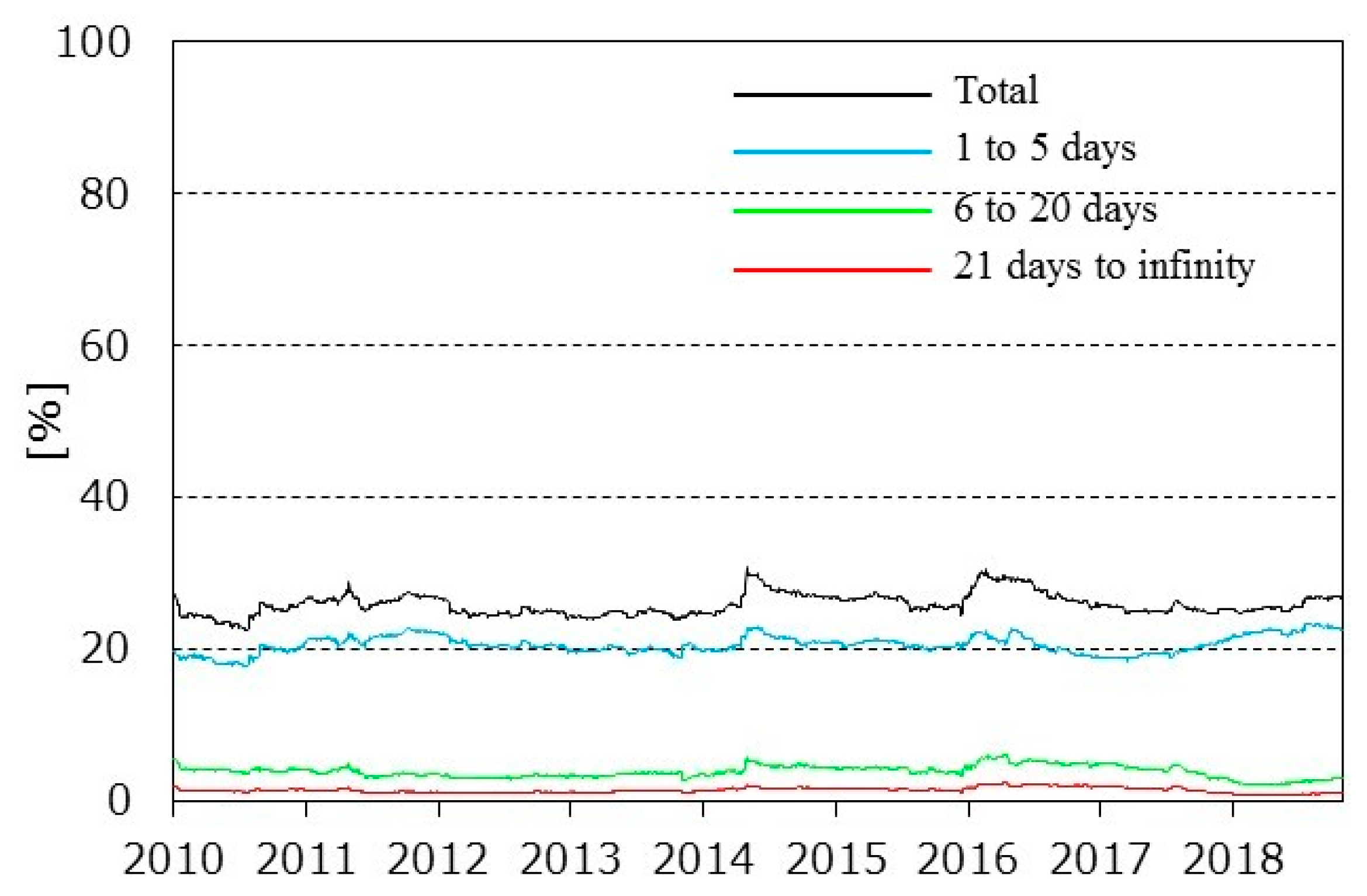
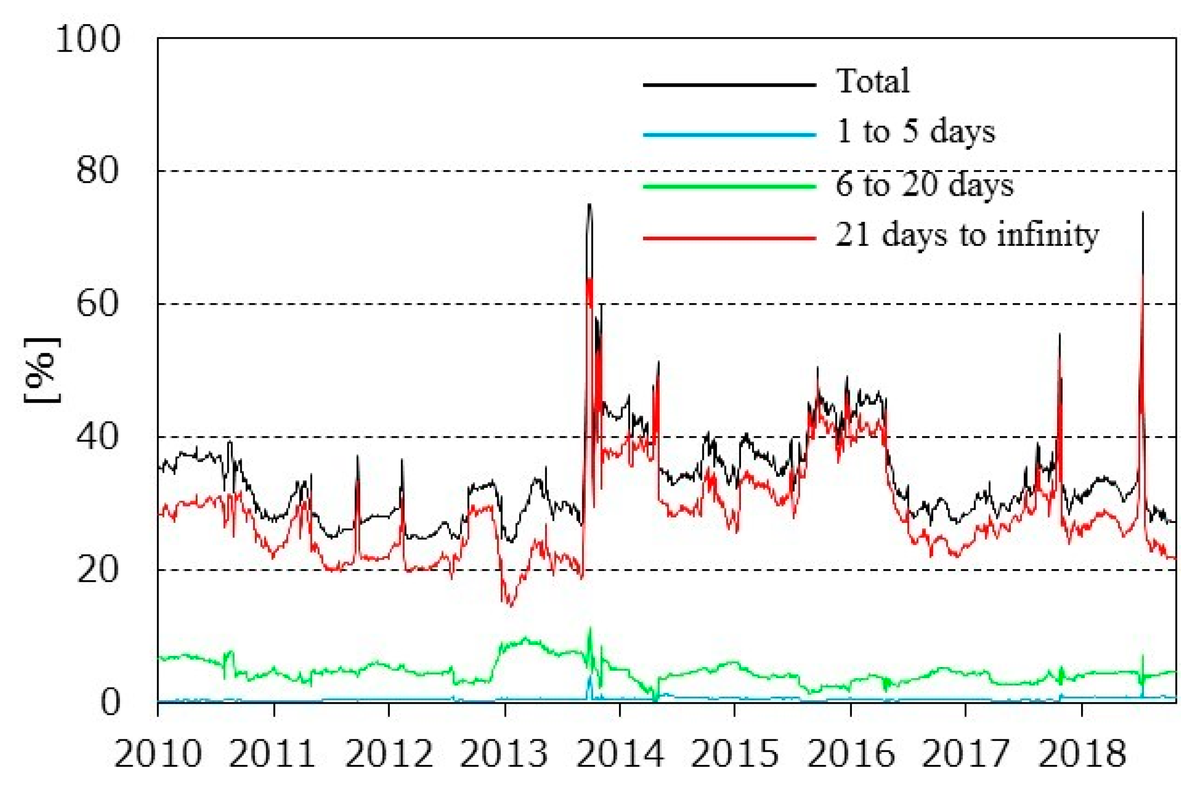
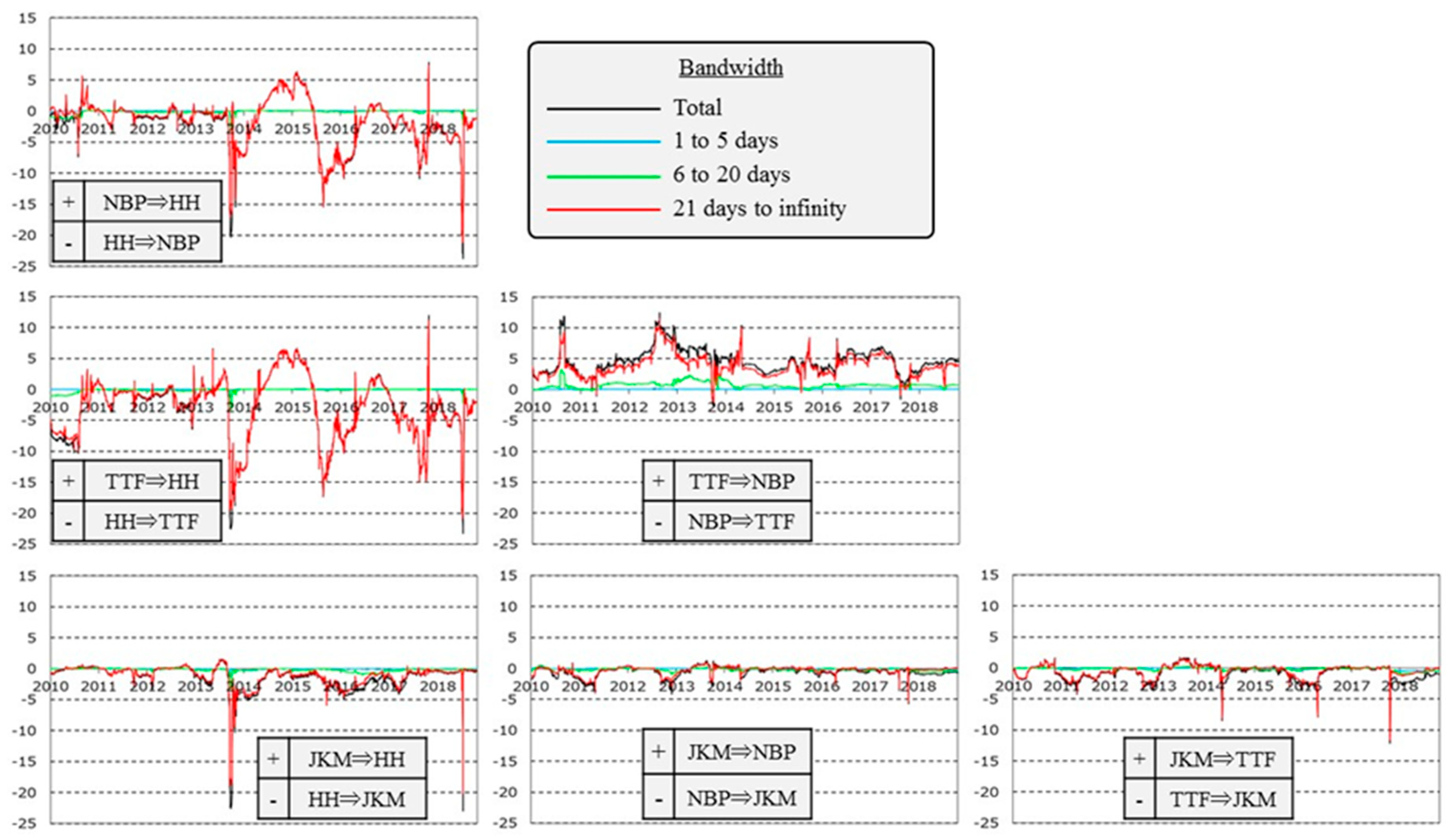
The results of the analyses for the entire period show that the total connectedness of return and volatility is 22.9% and 32.8%, respectively. Volatility is more highly integrated than returns in the global natural gas market. However, total connectedness is mostly dependent on the pairwise connectedness between NBP and TTF. Therefore, we cannot conclude that the global natural gas market is integrated.

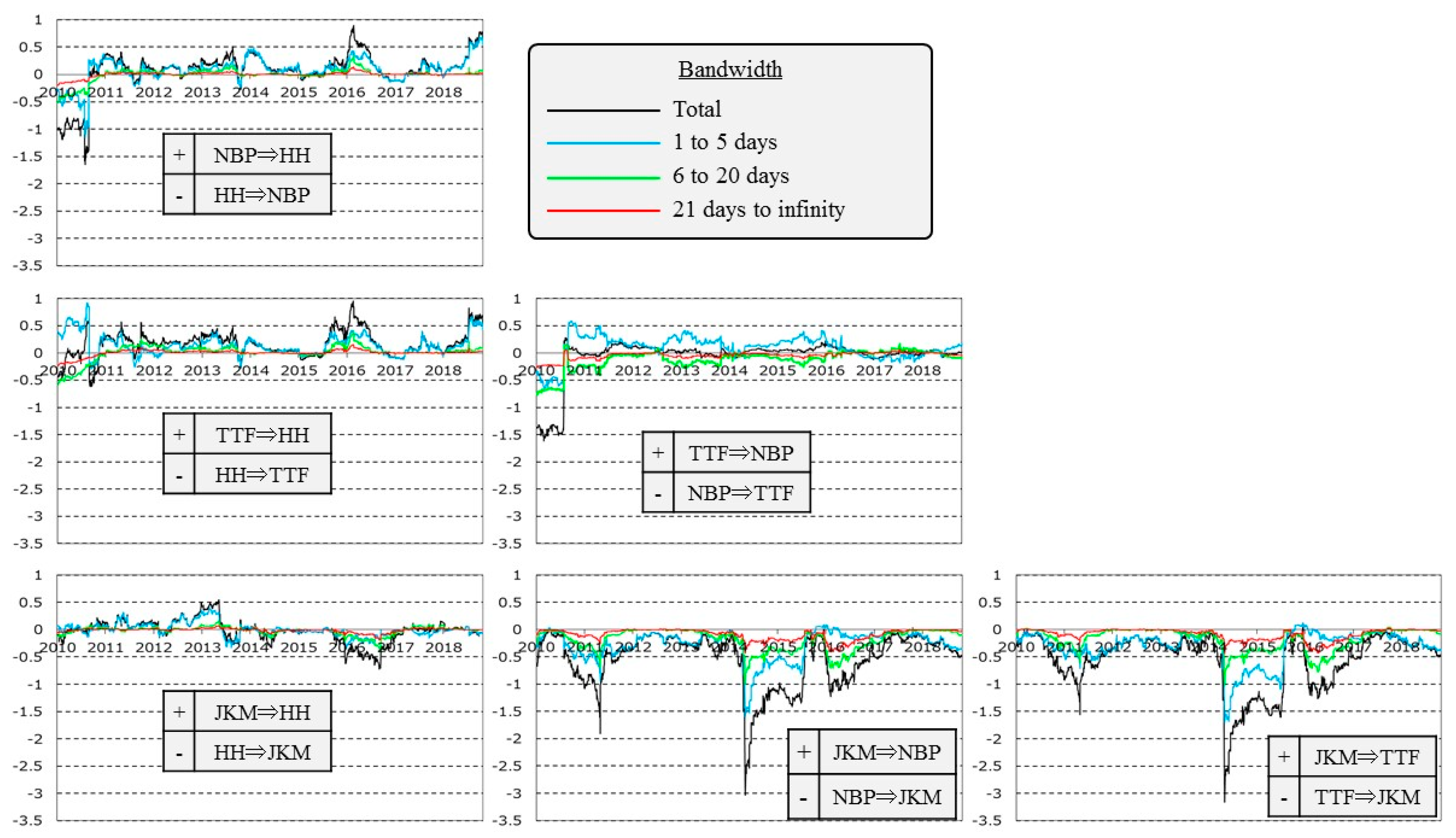
The results of the spectral analyses indicate that the spillover effects of the return series almost depend on short-term factors, that is, events within 5 business days. If we further expand the natural gas pipeline network to produce more LNG, the total connectedness of the return series and the ratio of short-term factors should be higher with the increase in arbitrage trading. By contrast, the spillover effect of the volatility series is almost dependent on the long-term factors, that is, accumulated shocks for more than a month. This result represents the long-term memory of volatility.

The results of the dynamic analyses with moving window samples are consistent with the results above. The spillover effects of the return and volatility series tend to be dependent on events within a week and more than a month ago, respectively. However, regional climate, demand and supply, and incidents might make spillover effects unstable. Unfortunately, the spillover index for around 10 years does not show that the liquidity of the global natural gas market tends to increase.

For practitioners, this study implies that constantly monitoring market spillovers is significant. The information obtained by this study’s approach is also of high value for energy portfolio rebalancing, including derivatives. Moreover, if we monitor the index as a predictive indicator, the information helps with early risk aversion.

Finally, clarification of the spillover effects between the crude oil and natural gas markets will be required for future studies, because many natural gas trading contracts still have their prices linked to crude oil prices.

References

- BP’s Statistical Review of World Energy. Available online: https://www.bp.com/en/global/corporate/energy-economics/statistical-review-of-world-energy.html (accessed on 29 September 2019).
- Japan Fair Trade Commission; Government of Japan. Ekika-Ten-Nen-Gas-No-Torihiki-Jittai-Ni-Kansuru-Chousa-Houkokusho (Survey on LNG Trades). 2017. Available online: https://www.jftc.go.jp/houdou/pressrelease/h29/jun/170628_1_files/170628_4.pdf (accessed on 29 September 2019).
- Diebold, F.X.; Yilmaz, K. Better to give than to receive: Predictive directional measurement of volatility spillovers. Int. J. Forecast. 2012, 28, 57–66. [Google Scholar] [CrossRef]
- Kum, H.; Ocal, O.; Aslan, A. The relationship among natural gas energy consumption, capital and economic growth: Bootstrap-corrected causality tests from G-7 countries. Renew. Sustain. Energy Rev. 2012, 16, 2361–2365. [Google Scholar] [CrossRef]
- Das, A.; McFarlane, A.A.; Chowdhury, M. The dynamics of natural gas consumption and GDP in Bangladesh. Renew. Sustain. Energy Rev. 2013, 22, 269–274. [Google Scholar] [CrossRef]
- Bildirici, M.E.; Bakirtas, T. The relationship among oil, natural gas and coal consumption and economic growth in BRICTS (Brazil, Russian, India, China, Turkey and South Africa) countries. Energy 2014, 65, 134–144. [Google Scholar] [CrossRef]
- Acaravci, A.; Ozturk, I.; Kandir, S.Y. Natural gas prices and stock prices: Evidence from EU-15 countries. Econ. Model. 2012, 29, 1646–1654. [Google Scholar] [CrossRef]
- Nakajima, T.; Hamori, S. Testing causal relationships between wholesale electricity prices and primary energy prices. Energy Policy 2013, 62, 869–877. [Google Scholar] [CrossRef]
- Atil, A.; Lahiani, A.; Nguyen, A.D. Asymmetric and nonlinear pass-through of crude oil prices to gasoline and natural gas prices. Energy Policy 2014, 65, 567–573. [Google Scholar] [CrossRef]
- Perifanis, T.; Dagoumas, A. Price and Volatility Spillovers Between the US Crude Oil and Natural Gas Wholesale Markets. Energies 2018, 11, 2757. [Google Scholar] [CrossRef]
- Tiwari, A.K.; Mukherjee, Z.; Gupta, R.; Balcilar, M. A wavelet analysis of the relationship between oil and natural gas prices. Resour. Policy 2019, 60, 118–124. [Google Scholar] [CrossRef]
- Xia, T.; Ji, Q.; Geng, J.B. Nonlinear dependence and information spillover between electricity and fuel source markets: New evidence from a multi-scale analysis. Physica A 2020, 537, 122298. [Google Scholar] [CrossRef]
- Batten, J.A.; Kinateder, H.; Szilagyi, P.G.; Wagner, N.F. Time-varying energy and stock market integration in Asia. Energy Econ. 2019, 80, 777–792. [Google Scholar] [CrossRef]
- Nakajima, T. Expectations for Statistical Arbitrage in Energy Futures Markets. J. Risk Financ. Manag. 2019, 12, 14. [Google Scholar] [CrossRef]
- Olsen, K.K.; Mjelde, J.W.; Bessler, D.A. Price formulation and the law of one price in internationally linked markets: An examination of the natural gas markets in the USA and Canada. Ann. Reg. Sci. 2015, 54, 117–142. [Google Scholar] [CrossRef]
- Scarcioffolo, A.R.; Etienne, X.L. How connected are the U.S. regional natural gas markets in the post-deregulation era? Evidence from time-varying connectedness analysis. J. Commod. Mark. 2019, 15, 100076. [Google Scholar] [CrossRef]
- Ren, X.; Lu, Z.; Cheng, C.; Shi, Y.; Shen, J. On dynamic linkages of the state natural gas markets in the USA: Evidence from an empirical spatio-temporal network quantile analysis. Energy Econ. 2019, 80, 234–245. [Google Scholar] [CrossRef]
- Nick, S. The informational efficiency of European natural gas hubs: Price formation and intertemporal arbitrage. Energy J. 2016, 37, 1–30. [Google Scholar] [CrossRef]
- Osička, J.; Lehotský, L.; Zapletalová, V.; Černoch, F.; Dančák, B. Natural gas market integration in the Visegrad 4 region: An example to follow or to avoid? Energy Policy 2018, 112, 184–197. [Google Scholar] [CrossRef]
- Bastianin, A.; Galeotti, M.; Polo, M. Convergence of European natural gas prices. Energy Econ. 2019, 81, 793–811. [Google Scholar] [CrossRef]
- Shi, X.; Shen, Y.; Wu, Y. Energy market financialization: Empirical evidence and implications from East Asian LNG markets. Financ. Res. Lett. 2019, 30, 414–419. [Google Scholar] [CrossRef]
- Neumann, A. World natural gas markets and trade: A multi-modeling perspective. Energy J. 2009, 30, 187–199. [Google Scholar] [CrossRef]
- Chai, J.; Wei, Z.; Hu, Y.; Su, S.; Zhang, Z.G. Is China’s natural gas market globally connected? Energy Policy 2019, 132, 940–949. [Google Scholar] [CrossRef]
- Silverstovs, B.; L’Hégaret, G.; Neumann, A.; Hirschhausen, C. International market integration for natural gas? A cointegration analysis of prices in Europe, North America and Japan. Energy Econ. 2005, 27, 603–615. [Google Scholar] [CrossRef]
- Baruník, J.; Křehlík, T. Measuring the frequency dynamics of financial connectedness and systemic risk. J. Financ. Econom. 2018, 16, 271–296. [Google Scholar] [CrossRef]
- Toyoshima, Y.; Hamori, S. Measuring the time-frequency dynamics of return and volatility connectedness in global crude oil markets. Energies 2018, 11, 2893. [Google Scholar] [CrossRef]
- Ji, Q.; Geng, J.B.; Tiwary, A.K. Information spillovers and connectedness networks in the oil and gas markets. Energy Econ. 2018, 75, 71–84. [Google Scholar] [CrossRef]
- Engle, R.F.; Kroner, K.F. Multivariate Simultaneous Generalized ARCH. Econom. Theory 1995, 11, 122–150. [Google Scholar] [CrossRef]
© 2019 by the authors. Licensee MDPI, Basel, Switzerland. This article is an open access article distributed under the terms and conditions of the Creative Commons Attribution (CC BY) license (http://creativecommons.org/licenses/by/4.0/).