Abstract
China’s industrial sector, which has a significant position in the world, is the main sector of China’s energy consumption and waste gas emission. China’s government has promulgated a Guiding Opinion, setting key regions to establish an emission reduction target of air pollutants during the 12th five year plan (2011–2015). Thus, there is a different regional treatment of industrial waste gas in China. This study considers the waste gas treatment expenditure as a new input and employs the non-radial directional distance function in the framework of the meta-frontier model to investigate the energy and emission reduction performance of China’s industrial sectors. The study is aimed at finding a significant and expanded technical gap between key and non-key regions in the energy and emission reduction efficiencies. The empirical result presents an effective method to improve the performance by increasing the emission treatment expenditure to reduce emissions.
1. Introduction
China is now the largest energy consumer in the world. According to Global Energy Statistical Yearbook 2017 [1], China’s total energy consumption reached 3.123 million TCE (tons of standard coal equivalent) in 2016, taking up about 55% of Asia’s energy consumption and nearly a quarter of the global consumption. Meanwhile, China is also the world’s largest emitter of CO2, the emissions of which in 2016 take up approximately 28.21% of the global total based on Statista [2]. Ke [3] evaluated the energy efficiency of APEC member economies over 18 consecutive years (1995–2012) and found China’s efficiency performance is relatively the worst, and indicated that a carbon reduction policy is more urgent and more important than an energy-saving policy in China.
In China, the industrial sector (containing mining, manufacturing, and power industries) is the main sector of energy consumption and CO2 emission. China’s industrial sector contributed 34.32% of the national GDP, while its share of China’s energy consumption was up to 67.98% [4]. The total waste gas emission of China’s industrial sector reached 68.52 trillion cubic meters [5]. Besides CO2, the industrial sector’s emissions also included SO2 (accounting for 83.73% of the country’s total), NOX (accounting for 63.79% of the country’s total), and soot (accounting for 66.59% of the country’s total).
At the same time, China’s industrial sector plays an important role in the world. Based on U.N. National Accounts Main Aggregates Database [6], China’s manufacturing industry, the main department of the industrial sector, achieved a value-add of 3.080 billion dollars in 2016, which was close to the total of the United States’ and Japan’s manufacturing industry, and exceeded one-quarter of the global manufacturing industry’s total. As a result, it is of great practical significance to take China’s industrial sector as a research object and analyze its energy and emission treatment efficiency, on which scholars should place particular emphasis.
The environmental issues caused by industrial emission, such as the greenhouse effect, acid rain, and haze, have become increasingly acute and attracted attention from the national government and society. China’s government has promulgated Guiding Opinions [7] in 2010 to deal with waste gas emission. The main line of the Guiding Opinions is to set key regions and establish an emission reduction target of air pollutants during the 12th five year plan (2011–2015) for cities in the key regions. The government measures in emission reduction for the key regions include installing waste gas treatment equipment like desulfurization, denitrification, and dust removal equipment in the industrial sector, imposing restrictions on high energy consumption industries that lead to air pollution (such as steel, cement, and glass industries), and accelerating the promotion of clean energy and new energy. The key regions include 14 provinces, as shown in Figure 1 below.
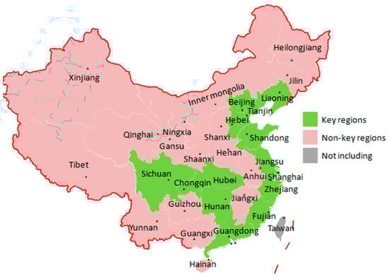
Figure 1.
Key and non-key regions under Guiding Opinions 2010.
In Figure 2, we compare the energy intensity between key and non-key regions using the proportion of energy consumption and revenue of China’s industry sector (unit: TCE per 100 million RMB) according to Energy Statistical Yearbook of China [8,9,10,11,12]. Similarly, the coal share of the total energy consumption (including coal, petroleum, natural gas, and electricity) is compared in Figure 3 using the proportion of coal in total energy consumption (unit: 100%), because coal is the main cause of waste gas emissions. As a result, a lower level and significant decrease trend can be found in the key regions from 2011–2015.
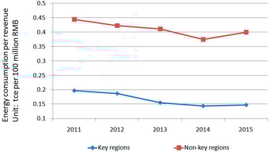
Figure 2.
Energy intensity between key and non-key regions.
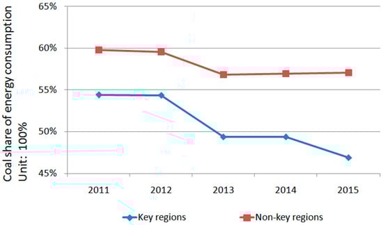
Figure 3.
Comparing coal share between key and non-key regions.
We find there is an increase of the treatment expenditure which can reduce emission in China’s industry sector from 2011–2015.Considering the efforts of emission reduction, we set up a new indicator called treatment intensity. The definition of treatment expenditure per cubic meter of emission is calculated by the proportion of expenditure of industrial waste gas treatment facilities (including desulfurization, de-nitrification, dust removal, etc.) and the volume of industrial waste gas emission (including CO2, SOx, NOx, soot, etc.), according to the China Statistical Yearbook on Environment [5,13,14,15,16]. The treatment intensity reflects the input level of waste gas treatment. The local economic development is crucial to treatment intensity, but the government policy is also considered as a common cause of regional differences. For instance, the average treatment intensity value from 2011–2015 of Hunan (2.91), Hubei (2.11), Sichuan (2.37), and Chongqing (2.38), which are key regions, is higher than that of Anhui (1.98), Henan (1.84), and Shaanxi (1.98), which are non-key regions, even though they have a similar economic development level. As shown in Figure 4, we find the increasing trend in both key and non-key regions. However, the treatment intensity in key regions is higher than that in non-key regions, despite the lower energy intensity and coal share in key regions. So we think there is difference between the regional treatment intensities of key and non-key regions, and the gap would not be filled in the next few years.
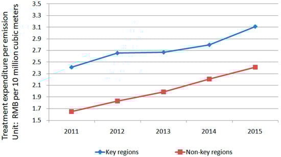
Figure 4.
Comparing treatment intensity between key and non-key regions.
Based on the background and analysis above, this study is aimed at investigating performance of energy and emission reduction of China’s industrial sector through employing the non-radial directional distance function in the framework of the meta-frontier model, and to divide China into key and non-key regions under the regional treatment differences.
Non-radial directional distance function is one kind of Data Envelopment Analysis (DEA). As for the DEA approach, a large number of studies apply radial DEA models, like the CCR model by Charnes et al. [17] and BCC model by Baker et al. [18]. But these models also ignore that most DMUs (Decision-Making Units) in business always want to maximize their profit. Chambers et al. [19] introduced a directional distance function that can estimate the efficiency scores by incorporating all types of inputs and outputs. The directional technology distance function generalizes radial measures in terms of input and output efficiency, because it allows the radial and non-radial increase of outputs and reduction of inputs. Besides, Färe and Grosskopf [20] pointed out that the directional technology distance function can be applied in an estimation of industrial inefficiency under the assumption that the resources can be efficiently allocated, whereas the directional technology distance function could be easily affected by the slack in the technological constraints. As mentioned by Färe and Lovell [21], efficiency measurement under an isoquant subset instead of an efficient subset may lead the unit’s identification to be technically efficient, while it is actually not. Therefore, many scholars pay attention to the non-radial models, such as Fukuyama and Weber [22,23], Färe and Grosskopf [24], Mahlberg and Sahoo [25], Zhou et al. [26], and Barros and Managi [27]. In this study, we employ the non-radial directional distance function, because non-radial DEA-based models seem to be more effective in estimating the industrial performance due to the higher discriminating power of non-radial efficiency measures in evaluating the efficiencies of DMUs.
The earliest application of DEA approach in energy and environment can be traced back to Färe et al. [28]. Using data from U.S. fossil-fuel-fired electric utilities, they established an environmental performance indicator through decomposing the overall factor productivity into a pollution index and an input-output efficiency index.
In the literature focusing on estimating and comparing the energy efficiency of macro economies by DEA, labor, capital, and energy consumption are widely accepted as inputs, and GDP and CO2, respectively, represent the desirable and undesirable outputs. This method first appeared in the comparison among OECD countries. For instance, Zaim et al. [29] used non-parametric techniques to build an environmental efficiency index for the OECD countries. Färe et al. [30] provided a formal index number of environmental performance using a sample of OECD countries for 1990.
Afterwards, this method was rapidly promoted internationally. The relevant follow-up literature position the following as the analysis objects: OECD (Zhou et al. [31], Zhou and Ang [32], Agergis et al. [33], Guo et al. [34]), APEC (Hu and Kao [35], Zhou et al. [36], Ke [3]), EU (Bampatsou et al. [37], Chang [38], Gómez-Calvet [39], Robaina-Alve et al. [40]), and BRICs (Song et al. [41]). In addition, there are many other studies applying this method to make comparisons between different countries, involving Ramanathan [42], Zhang et al. [43], Cui [44], and Jebali et al. [45].
With China’s economic growth, an increasing amount of research has been dedicated to examining the energy and emission efficiency of China. Hu and Wang [46] first used the above method of comparing countries to analyze energy efficiencies of 29 administrative regions in China from 1995 to 2002, considering labor, capital, and energy consumption as the three inputs, and GDP as the single output. Since then, many scholars have adopted similar input-output variables to compare the energy and emission efficiencies of China across different regions through DEA, such as Chang and Hu [47], Wu et al. [48], and Li and Lin [49].
Furthermore, CO2, a common concern of the world, was accepted as the undesirable output by several scholars and was introduced into the model to analyze China’s energy and emission efficiency (Choi et al. [50], Li and Hu [51], Wang et al. [52], Lin and Du [53]). Some other scholars introduced both CO2 and SO2, which are of more concern in China, into the efficiency model as the undesirable outputs (Yeh et al. [54], Wang and Feng [55], Zhang and Choi [56], Yu and Choi [57]).
Bettese et al. [58] and O’Donnell et al. [59] develop the meta-frontier model, which makes it possible to compare the performance of DMUs belonging to different contexts. This model decomposes the DMU’s attainment into its own management (efficiency) and technical gaps. It is assumed that all DMUs have potential access into a common frontier. Considering the regional disparities in China, some studies use Chinese provinces as DMUs to measure energy efficiency, under the assumption it is unrealistic and unfair that all provinces possess a consistent technology. So some scholars classified Chinese provinces into different groups, usually eastern, central, and western regions. Based on regional classification, they adopted the meta-frontier model to evaluate China’s energy efficiency and found that the technology efficiency gap between regional efficiencies is significant (Lin and Du [60], Wang et al. [61], Du et al. [62], Yao et al. [63]).
Some scholars have paid close attention to the energy and emission of China’s industrial sector. For instance, Cole et al. [64] found that China’s industrial emissions have a positive effect on energy use and human capital intensity and have a negative effect on productivity. Xu and Lin [65] derived that economic growth dictated the industrial CO2 emissions and its impact varied across regions. Then they also proposed policy recommendations to mitigate CO2 emissions in the manufacturing industry. Liu and Wang [66] applied network DEA to assess the energy efficiency of China’s provincial industrial sector by means of dividing the energy-producing department and energy-consuming department.
This study is different from the previous studies mentioned above, as follows. On the one hand, based on the traditional input-output variables, this paper adds expenditure of industrial waste gas treatment facilities as a new input variable affecting the emission reduction efficiency. Given that, the energy efficiency is revised and redefined as energy and emission reduction efficiencies in this paper. On the other hand, in contrast with previous studies, such as Lin and Du [60] and Wang et al. [61], which divided China into three groups (eastern, central, and western areas in China), this paper considers grouping under regional treatment differences, and applies the meta-frontier model to find the technical gap between key and non-key regions, making the results more convincing in evaluating the government’s efforts of emission reduction. Section 2 shows the methodology. Section 3 presents the empirical study. Section 4 offers discussion. Section 5 ends with conclusions and policy recommendation.
2. Methodology
2.1. Non-Radial Directional Distance Function
DEA has been heavily used in the past two decades on energy, environmental, and ecological efficiencies and productivity analysis. Farrell [67] firstly raised the concept of measuring efficiency with the production frontier, which has since been modified and expanded. Charnes et al. [17] extended the theoretical results of Farrell and applied them to multiple inputs and multiple outputs in a constant-returns-to-scale scenario. Banker et al. [18] incorporated the concept of a linear combination of convexity constraints and adjusted constant-returns-to-scale to variable-returns-to-scale. Both of them are able to measure radial efficiency, and it is assumed that the input and output variables are able to proportionally increase or decrease. Tone [68] then proposed a non-radial Slacks-Based Measure (SBM) to solve the problem that an input or output cannot be adjusted by an equal proportion in order to reach optimal efficiency.
Many of these conventional DEA methods, however, could not involve undesirable outputs. To introduce undesirable outputs to the DEA model, Luenberger [69] and Chung et al. [70] presented a radial directional output distance function, by extending the output distance function concept in Shephard’s input and output distance function. The radial directional output distance function provides both desirable and undesirable outputs under the same production basis, thus allowing one to analyze both increasing output and decreasing bad output.
According to Chung et al. [70], the directional distance function of the undesired output is expressed as follows:
Here, is the distance direction measured by the distance function. At the same time, the DMU requires increasing as a desirable output variable and decreasing as an undesirable output variable to achieve the productive production boundary.
The radial efficiency models neglect the variance of the variables, which may result in estimation errors. To overcome this defect, Färe and Grosskopf [24] set up a non-radial directional distance function, which is better compared with other methods because its estimation results are more reasonable and accurate. Other scholars have applied non-radial directional distance functions to assess energy and environmental efficiency analysis, such as Zhou et al. [26], Chiu et al. [50], Zhang and Choi [56], and Zhang et al. [71].
This study assumes that there are N provinces (N decision making units, DMUs), and each province employs four inputs of capital (K), labor (L), and energy (E) and expenditure (EX) to produce a desirable output of Revenue (R) and one undesirable output of Industrial waste gas emission (Em). The production technology set (T) is defined below (Färe et al. [72]).
The production technology follows the standard axioms of production theory (Färe et al. [72]). Here, T is usually considered as a closed and bounded set, which possesses finite inputs that produce finite outputs. In order to model joint-production technology, it is assumed that T possesses the properties of weak disposability and null jointness.
Färe and Grosskopf [24] established the radial directional distance function as the below Equation (2).
In Equation (2), g = ( represents the direction vector that is required to reduce energy and CO2 emissions and increase GDP, under the corresponding ratio of β = (). If , then Equation (2) allows for an increase of GDP and a reduction of both energy and CO2 emissions as much as possible by a common scalar . Since the non-radial directional distance function allows for a more flexible calculation of slacks, it has discrimination power to identify slacks of energy, CO2 emissions, and GDP compared to the radial directional distance function.
Following Färe and Grosskopf [24], Zhou et al. [26], and Zhang et al. [71], the non-radial directional distance function is expressed as below.
In Equation (3), is an intensity variable, β = () denotes a weight vector, and g = () denotes an explicit directional vector.
2.2. Meta-Frontier and Non-Radial Directional Distance Function
Hayami and Ruttan [73] first put forward that DMUs do not possess a common production technology due to the differences in geographic location, market condition, economic development, and some other factors. Battese and Rao [74] and Battese et al. [58] noted the comparison of the technical efficiency (TEE) between different groups is feasible through a meta-frontier model. In other word, the countries tend to have hetero production technology, which is the basic idea of the meta-frontier (Battese et al. [58], O’Donnell et al. [59]). But the DMUs evaluated are often supposed to have the same production technology level as the traditional DEA models, although they actually have heterogeneous technology because of diverse geographic locations, public policies, socio-economic level, etc. Hence, on account of the non-radial directional distance function (Färe and Grosskopf [24], Zhou et al. [26], and Zhang et al. [71]) and meta-frontier model (O’Donnell et al. [59]), the meta-frontier non-radial directional distance function model is set as Equation (4).
According toFäre and Grosskopf [24], Zhou et al. [26], and Zhang et al. [71], the value of can be obtained through the following DEA model.
Because the meta-frontier is an envelope curve of the group frontier, it has more reference objects and represents the best production frontier. Given this, the technical efficiency value under the Group Frontier Efficiency (GFE) is higher than that under the Meta-Frontier Efficiency (MFE). The Technical efficiency Gap Ratio (or technology gap ratio, TGR) is calculated from the ratio value of MFE to GFE, as Equation (5) showed.
3. Empirical Study
3.1. Data and Variables
When the previous studies assessed the energy efficiency through DEA, labor, capital, and energy consumption are generally taken as inputs, and GDP and CO2, respectively, refer to the desirable and undesirable outputs. As mentioned above, Guiding Opinions promulgated by the Chinese government in 2010 have a mandatory requirement that the enterprises in industrial sectors should achieve emission reduction targets during the 12th five year plan (2011–2015). We find that the number of industrial waste gas treatment facilities (i.e., facilities) in China’s industrial sector has increased obviously during the five years, and annual expenditure for operation of industrial waste gas treatment facilities (i.e., expenditure) also has a significant expansion. Figure 5 shows the trends of facilities and expenditure from 2011–2015.Aremarkable rise is found in revenue of China’s industrial sector from 2011–2015, while emission relatively maintains a stable level, as shown in Figure 6. So we believe expenditure has played a positive role in restraining the growth of emission but increase the company’s cost of input. This general trend provides an objective basis in introducing expenditure as a new input variable in this study.
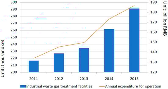
Figure 5.
The trends of facilities and expenditure from 2011–2015.
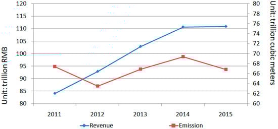
Figure 6.
Trends of revenue and emission from 2011–2015.
We list 30 of China’s provinces (except Tibet and Taiwan) as DMUs, collect data from 2011–2015 according to the Industry Statistical Yearbook of China [75,76,77,78,79], Energy Statistical Yearbook of China [5,13,14,15,16], and Statistical Yearbooks on Environment of China [8,9,10,11,12]. Variables are described as follows.
Input variables:
Annual average employees (Labor): Unit is one million persons.
Labor refers to the number of industrial companies’ employees in each province at the end of each year.
Total asset (Capital): Unit is one trillion RMB.
Capital represents the industrial companies’ total assets in each province.
Total energy consumption (Energy): Unit is one million TCE.
The coal, petroleum, natural gas, and electricity consumed by industrial companies are added together as total energy consumption of each province.
Expenditure of industrial waste gas treatment facilities (Expenditure): Unit is billion RMB.
Expenditure of industrial waste gas treatment facilities indicates the annual operating cost of waste gas treatment equipment, such as desulfurization, denitrification, and dust removal equipment.
Desirable output variable:
Revenue from principal business (Revenue): Unit is one trillion RMB
Revenue represents the main business income of industrial enterprises in each province.
Undesirable output variable:
Industrial waste gas emission (Emission): Unit is one trillion cubic meters.
Industrial waste gas emission represents the total emissions of CO2, SO2, NOX, and soot, which is measured by the volume of emissions.
Descriptive statistics of input and output variables is reported in Table 1.

Table 1.
Descriptive statistics of inputs and outputs.
3.2. Empirical Results
As shown in Figure 1, the key regions in Guiding Opinions 2010 contains 14 provinces, including Beijing, Tianjin, Hebei, Liaoning, Shanghai, Jiangsu, Zhejiang, Fujian, Shandong, Guangdong, Hubei, Hunan, Chongqing, and Sichuan. In response to this regional disparity, we divide the 30 DMUs into two groups, such as key regions and non-key regions.
Applying the non-radial Directional Distance Function (DDF) model, we estimate the energy and emission reduction efficiencies of 30 of China’s provinces (DMUs). In addition, it is worth pointing out that Slacks Based Measure (SBM) is another non-radial model, and we compare the results measured by DDF and SBM methods in Table 2. The distribution of average values measured by DDF and SBM methods are illustrated in Figure 7 and Figure 8.
Table 2.
Measured by Directional Distance Function (DDF) and Slacks Based Measure (SBM) from 2011–2015.
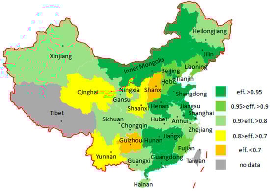
Figure 7.
Average values measured by DDF method from 2011 to 2015.
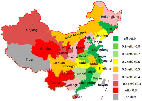
Figure 8.
Valuesmeasured by SBM method.
From Table 2, we find that the benchmark is mainly in the key regions, such as Beijing, Tianjin, Shanghai, Jiangsu, Shandong, and Guangdong. Only 2 DMUs, Jilin and Jiangxi, are the benchmark in the non-key regions. Comparing Figure 7 and Figure 8, we find the efficiency value measured by SBM is generally lower, because SBM looks for the farthest benchmark as room for improvement, and the room for improvement estimated by SBM is generally larger. On the contrary, DDF can take into account both desirable and undesirable outputs and find the optimal benchmark for improvement. Thus, we believe that the efficiency values estimated by DDF are more consistent with reality.
We find Sichuan, Chongqing, and Hubei, which are included in the key regions, have a clear trend of performance improvement during the five years. Particular emphasis should be placed on Hebei, Liaoning, and Zhejiang, the performance of which has decreased annually over the five years.
In non-key regions, Guangxi and Guizhou also show a distinct increase in their performance over the five years. However, the performances of DMUs is worse in 2015 than that in 2011, such as for Heilongjiang, Shanxi, Inner Mongolia, Shaanxi, Qinghai, and Xinjiang.
4. Discussion
4.1. The Technical Gap between Key Regions and Non-Key Regions
Based on the above estimates, it is already observed that there is a distinction of energy and emission reduction performances between the key and non-key regions. In this case, we further discuss whether the technical efficiency gap between the two regional groups is significant. The ratio of MFE to GFE is used to indicate the technical efficiency gap, as Equation (5) showed.
Table 3 shows the results of the DMUs’ MFE, GFE, and TGR in key and non-key regions. It presents that there is a different in efficiency and gaps in the country’s industries between the two regions. First, the country’s industries in key regions show outperforming efficiency, with 0.946 on average, compared with those in non-key regions (0.847) under the meta-frontier model. Second, turning to results under the group frontier, we find that the key regions have better performance, with an average value of 0.950, than those in non-key regions, with 0.887. This result indicates the DMUs in key regions are closer to their own frontier than those in non-key regions. It also means the DMUs in non-key regions have a higher technical gap, which can be inferred by the results of TGR. Third, the TGR of non-key regions has reached 0.940 in 2015, lower than that in 2011 (0.960), which reflects that there was an expansion of the gap between key and non-key regions from 2011 to 2015.
Table 3.
of MFE, GFE, and TGR from 2011–2015.
A wilcoxon score test is applied to further test the difference of the energy and emission treatment efficiencies between key and non-key regions. The p-value is compared with the confidence level αset as 0.01, 0.05, and 0.1, to testify whether there is significant distinction of TGR between two regional groups. From the results of the wilcoxon score test in Table 4, it shows that the p-values of the two groups’ average TGR are all less than α = 0.01 from 2011 to 2015, proving the average TGR between the two groups is distinct at the significance level of 99%.
Table 4.
Wilcoxon scorer test of technical efficiency gap.
From the above result, the energy saving and emission reduction policy for the key regions implemented by China’s government has achieved some success, but has simultaneously led to the significant efficiency gap between key and non-key regions. In the key regions, China’s government imposes restrictions on the high energy consumption industries and raises the requirement of installing emission reduction equipment in the companies, making the high energy consumption industries transferred into the non-key region. The transfer is an important reason accounting for the expansion of technical efficiency gap. To increase the overall energy and emission reduction efficiencies in the future, it should be an important goal for China to narrow the technical efficiency gap.
4.2. Room for Improvement of Energy and Emission Reduction Efficiencies
We estimate the room for improvement of 30 DMU inputs and outputs by using the non-radial directional distance function under the meta-frontier model, the results of which are in Table 5. We find that the country industrial sectors in key and non-key regions both have a larger room for improvement on the undesirable output variable (emission) than that on the input variable (energy and expenditure). It is vital to improve energy efficiency to mitigate global emissions, but this study indicates that the emission reduction effort is more important than an energy-saving effort in China’s industrial sector. On the other hand, to improve the over all performance, the effect of increasing expenditure, which can reduce emissions, is better than curbing expenditure, which can save cost.
Table 5.
Room for improvement of variables as average values from 2011–2015 unit: %.
Comparing the key and non-key regions, the biggest difference is reflected in the room for improvement in emission. For instance, the room for improvement in emission of Hubei, Hunan, Chongqing, and Sichuan (which are included in key regions but located in the central or western area of China) is significantly lower than DMUs with a similar level of economic development, such as Anhui, Henan, and Shaanxi. It is the reason why these 4 DMUs maintain high or increasing efficiency values. This is different from Lin and Du [60] and Wang et al. [61], who pointed out that the central and western area of China had lower energy efficiency.
However, 3 DMUs in key regions, containing Hebei, Liaoning, and Zhejiang, have decreasing energy and emission reduction efficiencies from 2011–2015. As the results show in Table 5, Hebei and Liaoning have a larger room for improvement in emission. We believe that it is related to the heavy industry transfer from Beijing and Tianjin. Zhejiang is the only one that has a larger room for improvement in expenditure among the 30 DMUs. Zhejiang should put more emphasis on the input of emission treatment expenditure, so as to avoid the company’s cost pressure caused by the rapid increase of treatment expenditure.
In the non-key regions, most DMUs have a gap between the room for improvement in emission and the other variables. To improve the performance of energy and emission reduction, a more effective method is needed to reduce emission by increasing the emission treatment expenditure, especially for DUMs with a lower room for improvement in expenditure, such as Heilongjiang, Anhui, Henan, and Shaanxi.
5. Conclusions and Policy Recommendation
China’s industrial sector is the main sector of China’s energy consumption and waste gas emission, which has a significant position in the world. Therefore, the energy and emission reduction performance of China’s industrial sector has attracted much attention from government and society. In 2010, the Chinese government released Guiding Opinions, where the industrial sector is the emphasis and key areas are set. In order to improve energy and emission reduction performance, the government has implemented an energy saving and emission reduction policy, and strengthened governance in the period of 2011–2015.
From the analysis results in this paper, we find DMUs in the key regions maintain a better performance, such as Beijing, Tianjin, Shandong, Jiangsu, Guangdong, and Hunan, or have significantly increasing efficiency values, such as Hubei, Chongqing, and Sichuan. Thus, we believe that the efforts made by the Chinese government have achievement some success. Meanwhile, the technical efficiency gap between key and non-key regions is significant and showed an expanded trend during 2011–2015. Instead of narrowing the technical efficiency gap, the setting of key areas is one of the reasons for the expansion of the gap. Given this, bridging the technical efficiency gap should become China’s future goal.
On the basis of the results in this study, it is argued that the level of treatment intensity of key regions is higher than that of non-key regions, which generally leads to better performance of emission reduction, such as Hubei, Hunan, Chongqing, and Sichuan in the central or western area of China. This is different from the results derived by Du [60] and Wang et al. [61], which indicate that DMUs in the central and western area of China have worse energy performance.
The main methods to improve the energy and emission reduction performance involve energy-saving, curbing expenditure of emission treatment, and reducing emission. We find that emission reduction efforts are more important than energy saving efforts in China’s industrial sector, and the effect of increasing expenditure on reducing emission is better than curbing expenditure. Thus, to improve the performance of energy and emission reduction, a more effective method is needed to reduce emission by increasing the emission treatment expenditure, especially for non-key regions, such as Hainan, Inner Mongolia, Guizhou, Gansu, Qinghai, Ningxia, and Xinjiang.
Author Contributions
Conceptualization, X.T. and Y.-h.C.; methodology, Y.-h.C.; software, X.T.; validation, X.T., D.L. and Y.-h.C.; formal analysis, X.T.; investigation, X.T.; resources, X.T.; data curation, X.T.; writing—original draft preparation, X.T.; writing—review and editing, D.L.; visualization, X.T.; supervision, Y.-h.C.; project administration, Y.-h.C.; funding acquisition, X.T.
Funding
This research received no external funding.
Conflicts of Interest
The authors declare no conflict of interest.
References
- Enerdata. Global Energy Statistical Yearbook. 2017. Available online: https://yearbook.enerdata.net/total-energy/world-consumption-statistics.html (accessed on 16 November 2018).
- Statista. Largest Producers of CO2 Emissions Worldwide in 2016, Based on Their Share of Global CO2 Emissions. 2017. Available online: https://www.statista.com/statistics/271748/the-largest-emitters-of-co2-in-the-world (accessed on 16 November 2018).
- Ke, T. Energy efficiency of APEC Members—Applied dynamic SBM model. Carbon Manag. 2017, 8, 293–303. [Google Scholar] [CrossRef]
- National Bureau of Statistics of China. China Statistical Yearbook. 2017. Available online: http://www.stats.gov.cn/tjsj/ndsj/2017/indexeh.htm (accessed on 16 November 2018).
- National Bureau of Statistics of China; National Bureau of Statistics Ministry of Environmental Protection. China Statistical Yearbook on Environment; China Statistics Press: Beijing, China, 2016.
- U.N. National Accounts Main Aggregates Database. Value Added by Economic Activity at Current Prices—U.S. Dollars. 2018. Available online: http://unstats.un.org/unsd/snaama/resQuery.asp (accessed on 16 November 2018).
- The State Council of China. Guiding Opinions about Promoting the Joint Prevention and Control of Air Pollution and Improving the Quality of the Public’s Living Environment. 2010. Available online: http://www.gov.cn/zwgk/2010-05/13/content_1605605.htm (accessed on 16 November 2018).
- National Bureau of Statistics of China; Department of Energy Statistical. China Energy Statistical Yearbook; China Statistics Press: Beijing, China, 2012.
- National Bureau of Statistics of China; Department of Energy Statistical. China Energy Statistical Yearbook; China Statistics Press: Beijing, China, 2013.
- National Bureau of Statistics of China; Department of Energy Statistical. China Energy Statistical Yearbook; China Statistics Press: Beijing, China, 2014.
- National Bureau of Statistics of China; Department of Energy Statistical. China Energy Statistical Yearbook; China Statistics Press: Beijing, China, 2015.
- National Bureau of Statistics of China; Department of Energy Statistical. China Energy Statistical Yearbook; China Statistics Press: Beijing, China, 2016.
- National Bureau of Statistics of China; National Bureau of Statistics Ministry of Environmental Protection. China Statistical Yearbook on Environment; China Statistics Press: Beijing, China, 2012.
- National Bureau of Statistics of China; National Bureau of Statistics Ministry of Environmental Protection. China Statistical Yearbook on Environment; China Statistics Press: Beijing, China, 2013.
- National Bureau of Statistics of China; National Bureau of Statistics Ministry of Environmental Protection. China Statistical Yearbook on Environment; China Statistics Press: Beijing, China, 2014.
- National Bureau of Statistics of China; National Bureau of Statistics Ministry of Environmental Protection. China Statistical Yearbook on Environment; China Statistics Press: Beijing, China, 2015.
- Charnes, A.; Cooper, W.W.; Rhodes, E. Measuring the efficiency of decision making units. Eur. J. Oper. Res. 1978, 2, 429–444. [Google Scholar] [CrossRef]
- Banker, R.D.; Charnes, A.; Cooper, W.W. Some models for estimating technical and scale inefficiencies in data envelopment analysis. Manag. Sci. 1984, 30, 1078–1092. [Google Scholar] [CrossRef]
- Chambers, R.G.; Fāure, R.; Grosskopf, S. Productivity growth in APEC countries. Pac. Econ. Rev. 1996, 1, 181–190. [Google Scholar] [CrossRef]
- Färe, R.; Grosskopf, S. Modeling undesirable factors in efficiency evaluation: Comment. Eur. J. Oper. Res. 2004, 157, 242–245. [Google Scholar] [CrossRef]
- Färe, R.; Lovell, C.K. Measuring the technical efficiency of production. J. Econ. Theory 1978, 19, 150–162. [Google Scholar] [CrossRef]
- Fukuyama, H.; Weber, W.L. A directional slacks-based measure of technical inefficiency. Socio-Econ. Plan. Sci. 2009, 43, 274–287. [Google Scholar] [CrossRef]
- Fukuyama, H.; Weber, W.L. A slacks-based inefficiency measure for a two-stage system with bad outputs. Omega 2010, 38, 398–409. [Google Scholar] [CrossRef]
- Färe, R.; Grosskopf, S. Directional distance functions and slacks-based measures of efficiency. Eur. J. Oper. Res. 2010, 200, 320–322. [Google Scholar] [CrossRef]
- Mahlberg, B.; Sahoo, B.K. Radial and non-radial decompositions of Luenberger productivity indicator with an illustrative application. Int. J. Prod. Econ. 2011, 131, 721–726. [Google Scholar] [CrossRef]
- Zhou, P.; Ang, B.W.; Wang, H. Energy and CO2 emission performance in electricity generation: A non-radial directional distance function approach. Eur. J. Oper. 2012, 221, 625–635. [Google Scholar] [CrossRef]
- Barros, C.P.; Managi, S.; Matousek, R. The technical efficiency of the Japanese banks: Non-radial directional performance measurement with undesirable output. Omega 2012, 40, 1–8. [Google Scholar] [CrossRef]
- Färe, R.; Grosskopf, S.; Tyteca, D. An activity analysis model of the environmental performance of firms—Application to fossil-fuel-fired electric utilities. Ecol. Econ. 1996, 18, 161–175. [Google Scholar] [CrossRef]
- Zaim, O.; Taskin, F. A Kuznets curve in environmental efficiency: An application on OECD countries. Environ. Resour. Econ. 2000, 17, 21–36. [Google Scholar] [CrossRef]
- Färe, R.; Grosskopf, S.; Hernandez-Sancho, F. Environmental performance: An index number approach. Resour. Energy Econ. 2004, 26, 343–352. [Google Scholar] [CrossRef]
- Zhou, P.; Poh, K.L.; Ang, B.W. A non-radial DEA approach to measuring environmental performance. Eur. J. Oper. 2007, 178, 1–9. [Google Scholar] [CrossRef]
- Zhou, P.; Ang, B.W. Decomposition of aggregate CO2 emissions: A production the oretical approach. Energy Econ. 2008, 30, 1054–1067. [Google Scholar] [CrossRef]
- Apergis, N.; Aye, G.C.; Barros, C.P.; Gupta, R.; Wanke, P. Energy efficiency of selected OECD countries: A slacks based model with undesirable outputs. Energy Econ. 2015, 51, 45–53. [Google Scholar] [CrossRef]
- Guo, X.; Lu, C.; Lee, J.; Chiu, Y. Applying the dynamic DEA model to evaluate the energy efficiency of OECD countries and China Energy. Energy 2017, 134, 392–399. [Google Scholar] [CrossRef]
- Hu, J.L.; Kao, C.H. Efficient energy-saving targets for APEC economies. Energy Policy 2007, 35, 373–382. [Google Scholar] [CrossRef]
- Zhou, D.Q.; Meng, F.Y.; Bai, Y.; Cai, S.Q. Energy efficiency and congestion assessment with energy mix effect: The case of APEC countries. J. Clean. Prod. 2017, 142, 819–828. [Google Scholar] [CrossRef]
- Bampatsou, C.; Papadopoulos, S.; Zervas, E. Technical efficiency of economic systems of EU-15 countries based on energy consumption. Energy Policy 2013, 55, 426–434. [Google Scholar] [CrossRef]
- Chang, M.C. Energy intensity, target level of energy intensity, and room for improvement in energy intensity: An application to the study of regions in the EU. Energy Policy 2014, 67, 648–655. [Google Scholar] [CrossRef]
- Gómez-Calvet, R.; Conesa, D.; Gómez-Calvet, A.R.; Tortosa-Ausina, E. On the dynamics of eco-efficiency performance in the European Union. Comput. Oper. Res. 2015, 66, 336–350. [Google Scholar] [CrossRef]
- Robaina-Alves, M.; Moutinho, V.; Macedo, P. A new frontier approach to model the eco-efficiency in European countries. J. Clean. Prod. 2015, 103, 562–573. [Google Scholar] [CrossRef]
- Song, M.L.; Zhang, L.L.; Liu, W.; Fisher, R. Bootstrap-DEA analysis of BRICS’ energy efficiency based on small sample data. Appl. Energy 2013, 112, 1049–1055. [Google Scholar] [CrossRef]
- Ramanathan, R. Estimating Energy Consumption of Transport Modes in India Using DEA and Application to Energy and Environmental Policy. J. Oper. Res. Soc. 2005, 56, 732–737. [Google Scholar] [CrossRef]
- Zhang, X.P.; Cheng, X.M.; Yuan, J.H.; Gao, X.J. Total-factor energy efficiency in developing countries. Energy Policy 2011, 39, 644–650. [Google Scholar] [CrossRef]
- Cui, Q.; Kuang, H.; Wu, C.; Li, Y. The Changing trend and influencing factors of energy efficiency: The case of nine countries. Energy 2014, 64, 1026–1034. [Google Scholar] [CrossRef]
- Jebali, E.; Essid, H.; Khraief, N. The analysis of energy efficiency of the Mediterranean countries: A two-stage double bootstrap DEA approach. Energy 2017, 134, 991–1000. [Google Scholar] [CrossRef]
- Hu, J.L.; Wang, S.C. Total-factor energy efficiency of regions in China. Energy Policy 2006, 34, 3204–3217. [Google Scholar] [CrossRef]
- Chang, T.P.; Hu, J.L. Total-factor energy productivity growth, technical progress, and efficiency change: An empirical study of China. Appl. Energy 2010, 87, 3262–3270. [Google Scholar] [CrossRef]
- Wu, A.H.; Cao, Y.; Lin, B. Energy efficiency evaluation for regions in China: An application of DEA and Malmquist indices. Energy Effic. 2014, 7, 429–439. [Google Scholar] [CrossRef]
- Li, K.; Lin, B. Metafroniter energy efficiency with CO2 emissions and its convergence analysis for China. Energy Econ. 2015, 48, 230–241. [Google Scholar] [CrossRef]
- Choi, Y.; Zhang, N.; Zhou, P. Efficiency and abatement costs of energy-related CO2 emissions in China: A slacks-based efficiency measure. Appl. Energy 2012, 98, 198–208. [Google Scholar] [CrossRef]
- Li, L.B.; Hu, J.L. Ecological total-factor energy efficiency of regions in China. Energy Policy 2012, 46, 216–224. [Google Scholar] [CrossRef]
- Wang, K.; Wei, Y.M.; Zhang, X. A comparative analysis of China’s regional energy and emission performance: Which is the better way to deal with undesirable outputs? Energy Policy 2012, 46, 574–584. [Google Scholar] [CrossRef]
- Lin, B.; Du, K. Energy and CO2 emissions performance in China’s regional economies: Do market-oriented reforms matter? Energy Policy 2015, 78, 113–124. [Google Scholar] [CrossRef]
- Yeh, T.; Chen, T.; Lai, P. A comparative study of energy utilization efficiency between Taiwan and China. Energy Policy 2010, 38, 2386–2394. [Google Scholar] [CrossRef]
- Wang, Z.; Feng, C. A performance evaluation of the energy, environmental, and economic efficiency and productivity in China: An application of global data envelopment analysis. Appl. Energy 2015, 147, 617–626. [Google Scholar] [CrossRef]
- Zhang, N.; Choi, Y. Environmental energy efficiency of China’s regional economies: A non-oriented slacks-based measure analysis. Soc. Sci. J. 2013, 50, 225–234. [Google Scholar] [CrossRef]
- Yu, Y.; Choi, Y. Measuring environmental performance under regional heterogeneity in China: A meta-frontier efficiency analysis. Comput. Econ. 2015, 46, 375–388. [Google Scholar] [CrossRef]
- Battese, G.E.; Rao, D.S.P.; O’Donnell, C.J. A metafrontier production function for estimation of technical efficiencies and technology gaps for firms operating under different technologies. J. Prod. Anal. 2004, 21, 91–103. [Google Scholar] [CrossRef]
- O’Donnell, C.J.; Rao, D.S.P.; Battese, G.E. Metafrontier frameworks for the study of firm-level efficiencies and technology ratios. Empir. Econ. 2008, 34, 231–255. [Google Scholar] [CrossRef]
- Lin, B.; Du, K. Technology gap and China’s regional energy efficiency: A parametric metafrontier approach. Energy Econ. 2013, 40, 529–536. [Google Scholar] [CrossRef]
- Wang, Q.; Zhao, Z.; Zhou, P.; Zhou, D. Energy efficiency and production technology heterogeneity in China: A meta-frontier DEA approach. Econ. Model. 2013, 35, 283–289. [Google Scholar] [CrossRef]
- Du, K.; Lu, H.; Yu, K. Sources of the potential CO2 emission reduction in China: Anon parametricmetafrontier approach. Appl. Energy 2014, 115, 491–501. [Google Scholar] [CrossRef]
- Yao, C.; Guo, C.; Shao, S.; Jiang, Z. Total-factor CO2 emission performance of China’s provincial industrial sector: A meta-frontier non-radial Malmquist index approach. Appl. Energy 2016, 184, 1142–1153. [Google Scholar] [CrossRef]
- Cole, M.; Elliott, R.; Wu, S. Industrial activity and the environment in China: An industry-level analysis. China Econ. Rev. 2008, 19, 393–408. [Google Scholar] [CrossRef]
- Xu, R.; Lin, B. Why are there large regional differences in CO2 emissions? Evidence from China’s manufacturing industry. J. Clean. Prod. 2017, 140, 1330–1340. [Google Scholar] [CrossRef]
- Liu, Y.; Wang, K. Energy efficiency of China’s industry sector: An adjusted network DEA (data envelopment analysis)-based decomposition analysis. Energy 2015, 93, 1328–1337. [Google Scholar] [CrossRef]
- Farrell, M.J.; PEARsoN, E.S. SERIES A (GENERAL). J. R. Stat. Soc. Ser. A (Gen.) 1957, 120, 229–253. [Google Scholar] [CrossRef]
- Tone, K. A slacks-based measure of efficiency in data envelopment analysis. Eur. J. Oper. Res. 2001, 130, 498–509. [Google Scholar] [CrossRef]
- Luenberger, D.G. New optimality principles for economic efficiency and equilibrium. J. Optim. Theory Appl. 1992, 75, 221–264. [Google Scholar] [CrossRef]
- Chung, Y.H.; Färe, R.; Grosskopf, S. Productivity and undesirable outputs: A directional distance function approach. J. Environ. Manag. 1997, 51, 229–240. [Google Scholar] [CrossRef]
- Zhang, N.; Zhou, P.; Choi, Y. Energy efficiency, CO2 emission performance and technology gaps in fossil fuel electricity generation in Korea: A meta-frontier non-radial directional distance function analysis. Energy Policy 2013, 56, 653–662. [Google Scholar] [CrossRef]
- Färe, R.; Grosskopf, S.; Pasurka, C.A., Jr. Environmental production functions and environmental directional distance functions. Energy 2007, 32, 1055–1066. [Google Scholar] [CrossRef]
- Hayami, Y.; Ruttan, V.W. Agricultural productivity differences among countries. Am. Econ. Rev. 1970, 60, 895–911. [Google Scholar]
- Battese, G.E.; Rao, D.P. Technology gap, efficiency, and a stochastic metafrontier function. Int. J. Bus. Econ. 2002, 1, 87–93. [Google Scholar]
- National Bureau of Statistics of China; Department of Industry Statistical. China Industry Statistical Yearbook; China Statistics Press: Beijing, China, 2012; Volume 1.
- National Bureau of Statistics of China; Department of Industry Statistical. China Industry Statistical Yearbook; China Statistics Press: Beijing, China, 2013; Volume 1.
- National Bureau of Statistics of China; Department of Industry Statistical. China Industry Statistical Yearbook; China Statistics Press: Beijing, China, 2014; Volume 1.
- National Bureau of Statistics of China; Department of Industry Statistical. China Industry Statistical Yearbook; China Statistics Press: Beijing, China, 2015; Volume 1.
- National Bureau of Statistics of China; Department of Industry Statistical. China Industry Statistical Yearbook; China Statistics Press: Beijing, China, 2016; Volume 1.
© 2019 by the authors. Licensee MDPI, Basel, Switzerland. This article is an open access article distributed under the terms and conditions of the Creative Commons Attribution (CC BY) license (http://creativecommons.org/licenses/by/4.0/).