Article

Charging–Discharging Control Strategy for a Flywheel Array Energy Storage System Based on the Equal Incremental Principle

1
Institute of Electrical Engineering, Chinese Academy of Sciences, Beijing 100190, China
2
University of Chinese Academy of Sciences, Beijing 100049, China
*
Author to whom correspondence should be addressed.
Energies 2019, 12(15), 2844; https://doi.org/10.3390/en12152844
Submission received: 27 June 2019 / Revised: 17 July 2019 / Accepted: 20 July 2019 / Published: 24 July 2019
(This article belongs to the Section D: Energy Storage and Application)

Abstract

:
The widely used flywheel energy storage (FES) system has such advantages as high power density, no environment pollution, a long service life, a wide operating temperature range, and unlimited charging–discharging times. The flywheel array energy storage system (FAESS), which includes the multiple standardized flywheel energy storage unit (FESU), is an effective solution for obtaining large capacity and high-power energy storage. In this paper, the strategy for coordinating and controlling the charging–discharging of the FAESS is studied in depth. Firstly, a deep analysis is conducted on the loss generated during the charging–discharging process of the FESU. The results indicate that the loss is related to the charging–discharging of power. To solve the problems of over-charging, over-discharging, and overcurrent caused by traditional charging–discharging control strategies, this paper proposes a charging–discharging coordination control strategy based on the equal incremental principle (EIP). This strategy aims to minimize the total loss and establish a mathematical model of optimal coordination control with the constraints of total charging–discharging power, rated power limit, over-charging, over-discharging, and overcurrent. Based on the EIP, the optimal distribution scheme of power charging–discharging is determined. Secondly, this paper gives the specific implementation scheme of the optimal coordinated control strategy. Lastly, the charging–discharging coordinated control strategy is verified by examples. The results show that the coordinated control strategy can effectively reduce the loss during the charging–discharging process and can prevent over-charging, over-discharging, and overcurrent of the system. Overall, it has a better control effect than the existing charging–discharging control strategies.

1. Introduction

To address the increasingly prominent environmental and energy problems, renewable energy sources, such as solar and wind energy, have developed rapidly in recent years. However, if renewable energy sources with characteristics of intermittence and randomness are connected to the power grid on a large scale, the voltage and frequency of the power grid will fluctuate drastically, resulting in poor continuity and stability of the power supply [1,2]. The configuration of a large capacity energy storage system in the power grid that utilizes charging and discharging functions can smooth out the power fluctuation in renewable energy, achieving decoupling control of both the power generation side and the power consumption side to improve the stability of the power grid [3]. At present, the energy storage form adopted in the power grid system is generally the storage battery, whose charging–discharging process is achieved by electrochemical reactions, with drawbacks such as slow speed, a limited recycling time, and a short service life. At the same time, the replacement of batteries will significantly increase operating costs [4]. In addition, wasted batteries pollute the environment.
Flywheel energy storage (FES) is a form of energy storage that uses a high-speed rotating flywheel rotor as a carrier to convert electrical energy into mechanical energy. It has the advantages of high power density, no environmental pollution, a long service life, and an almost unlimited charging–discharging time. Therefore, FES has been widely used in various fields, including renewable energy power generation, rail brake energy recovery, uninterrupted power supply (UPS), frequency modulation and voltage regulation in power systems, satellite energy storage, and attitude adjustment [5,6]. There are two main technical approaches used to acquire a larger storage capacity, higher charging–discharging power, and longer backup time. One is to develop a large-capacity single-unit FES system, and the other one is to connect multiple standardized flywheel energy storage units (FESUs) in parallel to form a flywheel array energy storage system (FAESS). The single large-capacity FES, however, not only increases the cost significantly but is also difficult to use due to technical limitations [3]. Comparatively, the FAESS can decrease both the cost and the time required for research and development; accordingly, it is a better solution for obtaining a high-capacity and high-power energy storage system.
Few studies have investigated the optimization of coordination control of the FAESS, both at home and abroad. In regard to charging, based on the average distribution algorithm, [7] proposes a distribution algorithm according to the chargeable capacity. As for discharging, discharging power distribution algorithms (average distribution, distribution by speed ratio, and distribution by residual energy ratio) are proposed in [7,8,9,10], and a preliminary simulation study was conducted. In terms of the FAESS used in wind farms, a layered distribution control strategy is presented in [11]: The upper layer is used to allocate energy to each FESU based on the proportional consistency algorithm, and the lower layer relies on the local controller in the FESU to adjust the rotating speed. This strategy, however, does not consider the effect of loss on the charging–discharging of the system. In [12], the FAESS is applied in the field of urban rail transit to absorb braking energy, and it achieves a good control effect; however, its power distribution scheme has not been studied in depth. The study presented in [13] advances a comprehensive electromechanical model of FES system, analyzes small-signal stability, and conducts time domain simulation research. The results show that the FAESS improves the stability of grid system, but the internal power distribution has not been studied in depth. In [14,15,16], an optimal control method aimed at FAESS is proposed for the grid-connected micro-grid. The upper optimization center establishes a corresponding charging–discharging optimized model according to the power vacancy and rotating speed of each flywheel, and solves the power parameter of each flywheel. The lower flywheel controller adopts a dual-module, dual-ring control method to control the rotating speed and output power of the flywheel. This method is still, essentially, a distribution by residual power ratio.
In general, the existing coordinated operation control of the FAESS mostly adopts the algorithms of average distribution, distribution by speed ratio, or residual energy ratio. These algorithms are likely to cause the distributed power to be greater than the available output power of the FESU, further causing overcurrent of the flywheel motor. At the same time, over-charging or over-discharging is likely to occur. In addition, the existing algorithms do not consider the internal loss factor of the system during the actual operation, resulting in low system operation efficiency. In order to solve these problems, further research on the FAESS is needed.
In this paper, the distribution of the charging–discharging power of the FAESS is studied in depth. Firstly, this paper conducts an in-depth analysis of the power loss of each component of the FESU, including the loss from the grid-side converter, the generator-side converter, and the motor. Then, with minimum loss as the optimization goal, an objective function of optimal control is established and solved by the equal incremental principle (EIP), with constraints on the total charging–discharging power, rated power limit, overcharging, over-discharging, and overcurrent. Secondly, based on theoretical research, a specific implementation scheme for the charging–discharging control strategy is proposed. Finally, the charging–discharging control strategy based on EIP is analyzed and verified by examples. The results demonstrate the effectiveness of the control strategy.

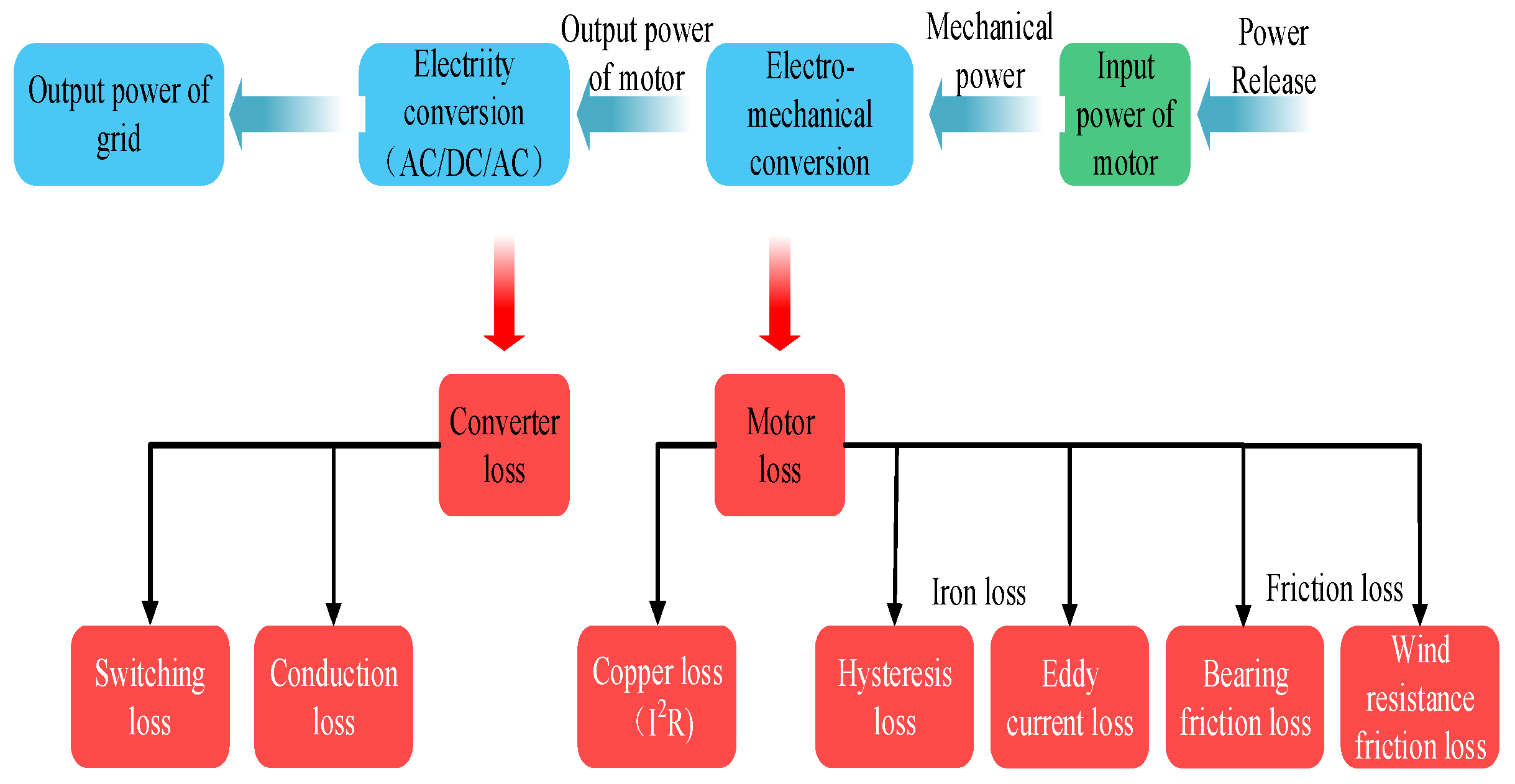
2. Loss Analysis of FESU

During charging, the FESU absorbs energy from the grid, whereas during discharge, it outputs energy into the grid. As shown in Figure 1, the converter generates switching and conduction loss during the power conversion process. During the electromechanical conversion process, the loss generated by the motor includes copper loss, iron loss (hysteresis loss, eddy current loss), and friction loss (bearing friction loss, wind resistance friction loss). When the FESU is connected to the grid for discharging, the loss distribution is as shown in Figure 2. The mechanical energy stored in the flywheel rotor is first converted into electrical energy through electromechanical conversion, and is then transferred into the power grid through the converter. Similar to that, during the charging process, the motor loss during the electromechanical conversion process includes copper loss, iron loss, and friction loss. During the process of power conversion, there are also switching and conduction losses.

2.1. Loss Analysis of the Converter in the FESU

The converter loss in the FESU includes the loss from the grid-side and the motor-side converters. As shown in Figure 3, taking the voltage source converter (VSC) as an example, the grid-side converter contains six insulated gate bipolar transistors (IGBTs) and six anti-parallel diodes, and the loss mainly includes switching and conduction loss. The switching loss in the grid-side converter is as shown in (1):
P s w _ G = 6 × ( P s w _ I G B T + P s w _ D ) = 6 π × f s w × ( E o n _ t e s t + E o f f _ t e s t + E r e c _ t e s t ) × I m I t e s t × U d c V t e s t
where P s w _ G represents the switching loss of the grid-side converter; P s w _ I G B T represents the switching loss of a single IGBT; P s w _ D represents the switching loss of a single diode; E o n _ t e s t represents the switching-on loss of the IGBT; E o f f _ t e s t represents the switching-off loss of the IGBT; E r e c _ t e s t represents the switching-off loss of the diode; I t e s t represents the test current; V t e s t represents the test voltage; I m represents the output current of the grid-side converter; U d c represents the DC bus voltage; and f s w represents the switching frequency of the grid-side converter.
Since the conduction loss of the negative half-cycle of the grid-side converter is the same as that of the positive half-cycle, we can only consider the conduction loss of the positive half-cycle. In the one-phase leg of the grid-side converter, the conduction loss of the IGBT is
P I G B T = V T 0 · I m ( 1 π + 1 4 m cos φ ) + R C E · I m 2 · ( 1 4 + 2 3 π m cos φ )
where P I G B T represents the conduction loss of the IGBT in the one-phase leg of the grid-side converter; V T 0 represents the IGBT threshold voltage; I m represents the output phase current in the grid-side converter; m represents the modulation ratio; φ represents the power factor angle; and R C E represents the IGBT conduction resistance.
By calculating the diode conduction loss, we can acquire
P D = V D 0 · I m ( 1 π 1 4 m cos φ ) + R D · I m 2 · ( 1 4 2 3 π m cos φ )
where P D represents the conduction loss of the diode in the one-phase leg of the grid-side converter; V D 0 represents the diode threshold voltage; I m represents the output phase current in the grid-side converter; m represents the modulation ratio; φ represents the power factor angle; and R D represents the diode conduction resistance.
The total conduction loss of grid-side converter P c o n d is
P c o n d = 3 ( P I G B T + P D ) = 3 I m · ( V T 0 + V D 0 π + m cos φ V T 0 V D 0 4 ) + 3 I m 2 · [ R C E + R D 4 + m cos φ 2 ( R C E R D ) 3 π ]
The absolute value of m cos φ is less than 1, and
| m   cos φ V T 0 V D 0 4 | < < V T 0 + V D 0 π
| m cos φ 2 ( R C E R D ) 3 π | < < R C E + R D 4
Therefore, the total conduction loss can be simplified to
P c o n d = 3 ( V T 0 + V D 0 ) π I m + 3 ( R C E + R D ) 4 I m 2 .
According to (1) and (7), the total conduction loss in the grid-side P G _ t o t is
P G _ t o t = b I m + c I m 2
b = 6 π × f s w × ( E o n _ t e s t + E o f f _ t e s t + E r e c _ t e s t ) × 1 I t e s t × U d c V t e s t + 3 ( V T 0 + V D 0 ) π
c = 3 ( R C E + R D ) 4 .
Since the relation between the amplitude of output phase current I m and the active power directive value P * is
I m = P * 3 U N × 2 ,
the total loss in the grid-side converter P G _ t o t is
P G _ t o t = d | P | + f P 2
where
d   =   b × 2 3 U N =   [ 6 π × f s w × ( E o n _ t e s t + E o f f _ t e s t + E r e c _ t e s t ) × 1 I t e s t × U d c V t e s t + 3 ( V T 0 + V D 0 ) π ] × 2 3 U N
f = c × 2 3 U N 2 = 3 ( R C E + R D ) 4 × 2 3 U N 2 .
Taking the VSC converter as an example for the motor-side converter, the loss mechanism is exactly the same. In the dq coordinate system, the d axis current i d is set to be 0, and then the amplitude of the output phase current is the absolute value | i q | of the q axis current i q . Similarly, the total loss in the motor-side converter P M _ t o t is
P M _ t o t = b | i q | + c i q 2 .

2.2. Motor Loss of FESU

As shown in Figure 2 and Figure 3, the motor loss in the FESU is mainly copper loss, iron loss, and friction loss. The cooper loss P c u in the motor is
P c u = 3 2 R s i q 2 = g i q 2
where
g = 3 R s 2
where R s is the resistance of the stator in the motor.
The iron loss of the permanent magnet synchronous motor includes hysteresis loss and eddy current loss. The iron loss can be represented by the equivalent iron loss resistor R c . The equivalent steady state circuit of the permanent magnet synchronous motor that includes the iron loss resistor R c is shown in Figure 4.
From Figure 4, we can acquire (13):
{ i c d = ω e L q i o q R c = k L q i o q i c q = ω e ( L d i o d + ψ f ) R c = k ( L d i o d + ψ f )
where i c d represents the d axis equivalent current of the equivalent iron loss current i c ; i c q represents the q axis equivalent current of the equivalent iron loss current i c ; ω e represents the electric angular speed of the motor; ψ f represents the excitation flux linkage of the motor permanent magnet; L d represents the d axis equivalent inductance of the motor; L q represents the q axis equivalent inductance of the motor; i o d represents the d axis equivalent current of the motor; and i o q represents the q axis equivalent current of the motor.
According to (13), the iron loss of motor P F e is
P F e = 3 2 ( i c d 2 + i c q 2 ) R c = 3 2 k p ω m [ ( L d i o d + ψ f ) 2 + ( L q i o q ) 2 ] .
From
{ i d = i c d + i o d = k L q i o q + i o d = 0 i q = i c q + i o q = k ( L d i o d + ψ f ) + i o q
we can acquire
{ i o d = k L q ( i q k ψ f ) 1 + k 2 L d L q i o q = i q k ψ f 1 + k 2 L d L q .
Bringing (16) into (14), we can acquire
P F e = ( k 1 i q 2 + k 2 i q + k 3 ) × ω m
where ω m is the mechanical angular speed of the flywheel rotor and
k 1 = 3 2 k p ( 1 + k 2 L d 2 ) L q 2 ( 1 + k 2 L d L q ) 2 k 2 = 3 k 2 p ψ f ( L d L q ) L q ( 1 + k 2 L d L q ) 2 k 3 = 3 2 k p ( 1 + k 2 L q 2 ) ψ f 2 ( 1 + k 2 L d L q ) 2
The friction loss of the flywheel P f r can be represented by
P f r = B × ω m 2
where B represents the viscous friction coefficient and ω m represents the mechanical angular speed of the flywheel rotor.

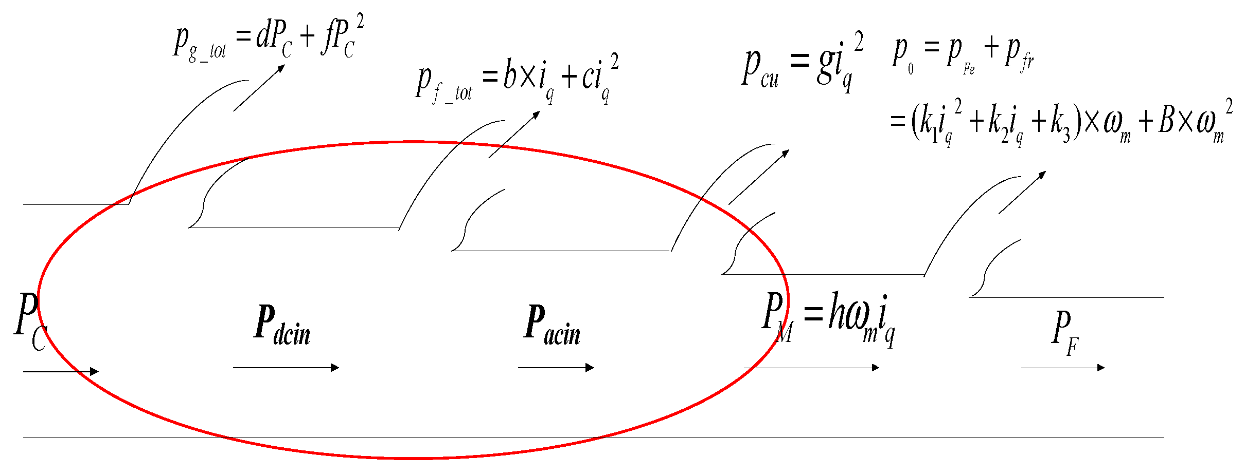
2.3. Analysis of the Total Charging–Discharging Loss of the FESU

Figure 5 shows the energy flowing when the FESU is charging. P C is the absolute value of the directive value of active power during charging; P d c i n is the DC input power of the generator-side converter; P a c i n is the AC output power of the generator-side converter; P M is the electromagnetic power of the flywheel motor; and P F is the actual storage power of the flywheel. During charging in the grid, the total loss P l o s s i n of FESU is
P l o s s i n = α P C 2 + β P C + γ
where
α = f + ( c + g + k 1 ω m ) k ω 2
β = d + ( b + k 2 ω m ) k ω
γ = k 3 ω m + B ω m 2 .
The energy flowing in the FESU during discharge is shown is Figure 6. P D is the absolute value of the directive value of active power during discharge; P d c o u t is the DC output power of the motor-side converter; P a c o u t is the AC input power of the motor-side converter; P M is the electromagnetic power of the flywheel motor; and P F is the actual output power of the flywheel. During charging of the grid, the total loss P l o s s o u t of FESU is
P l o s s o u t = α P D 2 + β P D + γ
where
α = f + ( c + g + k 1 ω m ) k ω 2
β = d + ( b + k 2 ω m ) k ω
γ = k 3 ω m + B ω m 2 .
It can be seen from the above analysis that when the FESU is charged or discharged, the generated loss is related to power charging or discharging. In the case that the total charging or discharging power is fixed, the charging or discharging power that distributes to each unit is different and so is the generated loss and the total loss in the system. Therefore, it is necessary to conduct in-depth research on the charging–discharging coordination control strategy of the FAESS.

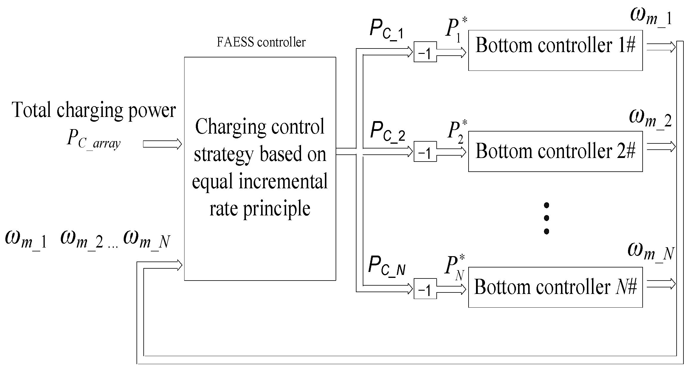
3. Charging Control Strategy of the FAESS

3.1. Charging Objective Function for the FAESS

When the total charging power of the system is fixed, in order to minimize the total loss P l o s s _ t o t during the charging operation, the objective function is as follows:
P l o s s _ t o t = i = 1 N P l o s s _ i ( P C _ i )
P l o s s _ i ( P C _ i ) = α i P C _ i 2 + β i P C _ i + γ i   ( i = 1 , 2 , , N )
where P l o s s _ t o t represents the total loss of the FAESS during charging; P l o s s _ i represents the loss of FESU i during charging; P C _ i represents the charging power reference value of FESU i; and
α i = f + ( c + g + k 1 ω m _ i ) k ω _ i 2
β i = d + ( b + k 2 ω m _ i ) k ω _ i
γ i = k 3 ω m _ i + B ω m _ i 2
k ω _ i = 1 d b + h ω m _ i .

3.2. Charging Constraints of FAESS

3.2.1. Equity Constraint

The sum of the total charging power of FESU is equal to the charging power reference value of the system P C _ a r r a y , which is
i = 1 N P C _ i = P C _ a r r a y .

3.2.2. Inequity Constraints

(1) Inequity constraints of the limited amplitude of the rated power
The charging power of each FESU cannot exceed its rated power, which is
0 P C _ i P r a t e d      ( i = 1 , 2 , , N ) .
(2) Inequity constraints of overcharging prevention
The current rotating speed of FESU i is set as ω m _ i , and the kinetic energy is set as E i . After operating cycle Δ T , the rotating speed is changed to ω m _ i _ n e x t and the kinetic energy is changed to E i _ n e x t . In order to prevent overcharging, the rotating speed of the next moment ω m _ i _ n e x t should not exceed the maximum permitted rotating speed ω m a x , as shown in Figure 7.
The kinetic energy of the flywheel energy storage unit at the next moment E i _ n e x t should not exceed the maximum allowable kinetic energy E m a x (25).
E i _ n e x t = E i + P F _ i × Δ T E m a x
where P F _ i is the current input power of i of the flywheel rotor.
Equation (25) can be represented by
P F _ i P C _ i d P C _ i f P C _ i 2 B ω m _ i 2 .
According to (26),
E i + P F _ i × Δ T E i + ( P C _ i d P C _ i f P C _ i 2 B ω m _ i 2 ) × Δ T .
It can be seen from (27) and (25) that if (28) is established, (25) is also established:
E i + ( P C _ i d P C _ i f P C _ i 2 B ω m _ i 2 ) × Δ T E m a x .
From (28), (29) is acquired:
1 2 J ω m _ i 2 + ( P C _ i d P C _ i f P C _ i 2 B ω m _ i 2 ) × Δ T 1 2 J ω m a x 2 .
which is
f · Δ T · P C _ i 2 + l · Δ T · P C _ i + 1 2 J ω m a x 2 1 2 J ω m _ i 2 + B · Δ T · ω m _ i 2 0
where l = d 1 and
A i = 1 2 J ω m a x 2 1 2 J ω m _ i 2 + B · Δ T · ω m _ i 2 .
Then,
f · Δ T · P C _ i 2 + l · Δ T · P C _ i + A i 0 .
According to (32),
P C _ i l · Δ T ( l · Δ T ) 2 4 A i f · Δ T 2 f · Δ T = P O C h _ i _ m a x      ( i = 1 , 2 , , N )
where for A i , as in (31), l = d 1 .
Equation (33) is the constraint for preventing the overcharging of FESU i.
(3) Inequity constraints of preventing overcurrent in the motor
If the distributed charging power is excessive, overcurrent can occur in the flywheel motor when the FESU is connected to the grid and charging. The q axis current of flywheel motor i is set as i q _ i . After operating cycle Δ T , the q axis current in the next moment will be i q _ i _ n e x t . Since the charging power is constant and the rotating speed is increasing within operating cycle Δ T , there will be i q _ i _ n e x t < i q _ i , as shown in Figure 8. In order to prevent the overcurrent of flywheel motor i , the q axis current i q _ i cannot exceed the maximum permitted q axis current i q _ m a x . Thus, the q axis current will naturally not exceed i q _ m a x , so (34) should be guaranteed:
i q _ i i q _ m a x .
According to (34),
i q _ i = k ω _ i P C _ i i q _ m a x
and then,
P C _ i i q _ m a x / k ω _ i = P O C u r _ i _ m a x
where
k ω _ i = ( 1 d ) / ( b + h ω m _ i )
h = 3 p ψ f 2 .
Equation (38) is the constraint for preventing the overcurrent of flywheel motor i .
According to (24), (33), and (36), the upper limit of charging power should be the minimum of these three values, which is
P C _ i _ m a x = min ( P r a t e d , P O C h _ i _ m a x , P O C u r _ i _ m a x )    ( i = 1 , 2 , , N ) .
Comprehensively, when the FAESS is charging, the charging power of each unit should meet the following inequality constraints:
0 P C _ i P C _ i _ m a x    ( i = 1 , 2 , , N ) .

3.3. Research of the Charging Control Method for FAESS

The charging power distribution of FAESS can be presented with the equality constraint of
i N P C _ i = P C _ a r r a y .
Let the objective function:
P l o s s _ t o t = i = 1 N P l o s s _ i ( P C _ i )
be the minimum, where p l o s s _ i ( P C _ i ) = α i P 2 C _ i + β i P C _ i + γ i represents the loss characteristics of each FESU during charging.
At the same time, the charging power of each unit P C _ i should also meet the following inequity constraints (38). When the minimum loss of the charging operation of the system is calculated by EIP, the LaGrange function shown in (41) should be constructed according to Objectives (39) and (40):
L = P l o s s _ t o t λ ( i = 1 N P C _ i P C _ a r r a y )
where λ represents the LaGrange multiplier.
The necessary condition for LaGrange function L to take the extreme value is
{ L P C _ i = P l o s s _ t o t P C _ i λ = 0      ( i = 1 , 2 , , N ) i = 1 N P C _ i P C _ a r r a y = 0 .
The charging loss P l o s s _ i ( P C _ i ) of each unit is only the function that relates to its charging power P C _ i ; therefore,
p l o s s _ t o t P C _ i   =   d p l o s s _ i ( P C _ i ) d P C _ i   =   2 α i P C _ i + β i = λ i      ( i = 1 , 2 , , N )
where λ i represents the incremental rate of consumption of each FESU.
Equation (42) can be rewritten as
{ 2 α i P C _ i + β i = λ      ( i = 1 , 2 ,   ,   N ) i = 1 N P C _ i P C _ a r r a y = 0 .
There are N + 1 equations and N + 1 variables in (44), which means the value of P C _ i solved by (44) is the value of distributed charging power with minimum loss.
When the charging power of FESU i is lower than the lower limit or higher than the upper limit, the charging power of the system will be zero or P C _ i _ m a x . Then, the residual charging power will be distributed to other FESUs.

3.4. Implementation Scheme of Charging Control for FAESS

After the calculation of the distributed power value corresponding to the minimum loss based on the equal incremental principle, the directive charging order will be sent to each underlying controller to realize coordinated charging control of each unit. As shown in Figure 9, the implementation consists of an array controller and N bottom controllers. The array controller runs the charging coordinated control strategy based on the EIP and outputs the most optimal charging power value corresponding to the minimum loss; each bottom controller will control the charging process of each unit by following the distributed charging power.
The main steps of the coordination control strategy based on EIP are as follows:
(1) The directive value of the total charging power P * a r r a y and the rotating speed of each flywheel ω m _ i are sampled and systematic parameters are invoked.
(2) The upper limit of charging power is calculated to prevent overcharging and overcurrent of FESU, P O C h _ i _ m a x , and P O C u r _ i _ m a x .
(3) The upper charging power limit of each FESU, P C _ i _ m a x , is determined according to (36).
(4) Coefficients, α i , β i , and γ i are calculated using the quadratic equation of charging loss of FESU, P l o s s _ i ( P C _ i ) .
(5) The minimum and maximum values of the incremental ratio of charging consumption of each FESU, λ i , are determined:
{ λ i _ m i n = β i λ m a x = = 2 α i P C _ i _ m a x + β i .
(6) The minimum and maximum values of the incremental ratio of public consumption of the FAESS are determined:
{ λ m i n = min ( λ 1 _ m i n , λ 2 _ m i n , , λ N _ m i n ) λ m a x = max ( λ 1 _ m a x , λ 2 _ m a x , , λ N _ m a x ) .
(7) The incremental ratio of public consumption is set as λ ( 0 ) = λ m a x .
(8) The charging power P C _ i ( 0 ) corresponding to λ ( 0 ) is calculated using
P C _ i ( 0 ) = λ ( 0 ) β i 2 α i      ( i = 1 , 2 , , N ) .
If P C _ i ( 0 ) is over the limit, then the limit value is used.
(9) The deviation between the sum of charging power and the total charging power P C _ a r r a y corresponding to λ ( 0 ) is calculated:
Δ P C ( 0 ) = i = 1 N P C _ i ( 0 ) P C _ a r r a y .
(10) Verification of whether the power deviation will satisfy the permitted range is carried out using
Δ P C ( 0 ) ε .
If (49) is satisfied, then P C _ i ( 0 ) is the value of distributed charging power with minimum loss, then P i is given a negative value of P C _ i ( 0 ) as the directive value of the charging power of the FESU.
(11) If it is not satisfied, and λ ( 0 ) > λ m i n , then
λ ( 1 ) > λ ( 0 ) Δ λ .
The iterative computations start from step (8) until the power deviation satisfies the permitted range, or until the incremental ratio of public consumption is lower than or equal to λ m i n .
The charging coordination control program based on EIP is shown in Figure 10.

4. Discharging Control Strategy of the FAESS

4.1. Discharging Objective Function for the FAESS

When the FAESS is discharging, the loss P l o s s _ i of FESU i is related to its active discharging power P D _ i . In the case that the total discharging power is fixed, the distributed power of FESU i P D _ i is different, and so is its loss P l o s s _ i and the total loss of the system. With a fixed total discharging power, in order to minimize the total loss P l o s s _ t o t , the objective function is defined as follows:
p l o s s _ t o t = i = 1 N p l o s s _ i ( P D _ i )
P l o s s _ i ( P D _ i ) = α i P D _ i 2 + β i P D _ i + γ i    ( i = 1 , 2 , , N )
where
α i = f + ( c + g + k 1 ω m _ i ) k ω _ i 2
β i = d + ( b + k 2 ω m _ i ) k ω _ i
γ i = k 3 ω m _ i + B ω m _ i 2
k ω _ i = 1 + d b h ω m _ i .

4.2. Discharging Constraints of the FAESS

4.2.1. Equity Constraints

When the system is discharged, the equity constraint is that the sum of the discharging power of FESUs is equal to the total discharging power of the system P D _ a r r a y , which is
i = 1 N P D _ i = P D _ a r r a y .

4.2.2. Inequity Constraints

(1) Inequity constraint of the limited amplitude of the rated power
The discharging power of each unit cannot exceed its rated power, which is
0 P D _ i P r a t e d      ( i = 1 , 2 , , N ) .
(2) Inequity constraint of preventing over-discharging
The current rotating speed of FESU i is set as ω m _ i and the kinetic energy is set as E i . After operating cycle Δ T , the rotating speed is changed to ω m _ i _ n e x t and the kinetic energy is changed to E i _ n e x t . In order to prevent over-discharging, the rotating speed of the next moment ω m _ i _ n e x t should not be lower than the minimum permitted rotating speed ω m i n , as shown in Figure 11.
The kinetic energy of FESU in the next moment E i _ n e x t should be higher than its minimum limit E m i n , and Equation (55) should be guaranteed:
E i _ n e x t = E i P F _ i × Δ T E m i n .
In (55), P F _ i represents the current output power of flywheel rotor i :
P F _ i P D _ i + d P D _ i + f P D _ i 2 + B ω m _ i 2 .
According to (55) and (56),
E i E m i n + ( P D _ i + d P D _ i + f P D _ i 2 + B ω m _ i 2 ) × Δ T
which is
1 2 J ω m _ i 2 1 2 J ω m i n 2 + ( P D _ i + d P D _ i + f P D _ i 2 + B ω m _ i 2 ) × Δ T .
From (58), (59) is acquired:
f × Δ T × P D _ i 2 + e × Δ T × P D _ i + A i 0 ,  
and (60) can be acquired from (59):
P D _ i e × Δ T + ( e × Δ T ) 2 4 A i f × Δ T 2 f × Δ T = P O D c h _ i _ m a x
where
A i = B × Δ T × ω m _ i 2 + 1 2 J ω m i n 2 1 2 J ω m _ i 2
e = 1 + d .
Equation (60) is the constraint for the prevention of over-discharge of i FESU.
(3) Inequity constraints of preventing overcurrent of motor
If the distributed charging power is excessive, overcurrent of the flywheel motor can occur when FESU is connected to the grid and discharging. The q axis current of flywheel motor i as i q _ i is set. After operating cycle Δ T , the q axis current in the next moment will be i q _ i _ n e x t . Since it is within operating cycle Δ T , where the discharging power is constant and the rotating speed is decreasing, the absolute value of the q axis current at the next moment will be greater than the absolute value of the q axis current. In order to prevent overcurrent in flywheel motor i , the absolute value | i q _ i _ n e x t | of the q axis current in the next moment cannot exceed the maximum permitted q axis current i q _ m a x , as shown in Figure 12.
During discharging, there is
1 2 J ω m _ i _ n e x t 2 E i P D _ i × Δ T 1 ω m _ i _ n e x t J 2 ( E i P D _ i × Δ T )
and
h ω m _ i _ n e x t | i q _ i _ n e x t | P D _ i | i q _ i _ n e x t | P D _ i h ω m _ i _ n e x t .
From (61) and (62) we can acquire
| i q _ i _ n e x t | P D _ i h × J 2 ( E i P D _ i × Δ T )
and
i q _ m a x | i q _ i _ n e x t | .  
Therefore,
i q _ m a x P D _ i h × J 2 ( E i P D _ i × Δ T )
which is
J P D _ i 2 + 2 i 2 q _ m a x h 2 × Δ T × P D _ i i 2 q _ m a x h 2 J ω m _ i 2 0 .  
From (66), we can acquire
P D _ i i 2 q _ m a x h 2 × Δ T + i 4 q _ m a x h 4 Δ T 2 + J 2 i 2 q _ m a x h 2 ω m _ i 2 J = P O C u r _ i _ m a x      ( i = 1 , 2 , , N ) .  
Equation (67) is the constraint for preventing the overcurrent of FESU i .
According to (54), (60), and (67), the upper limit of the discharging power of FESU i should be the minimum of these three equations, which is
P D _ i _ m a x = min ( P r a t e d , P O D c h _ i _ m a x , P O C u r _ i _ m a x ) .  
Generally, when the FAESS is discharged, the discharging power of each unit should meet the following inequity constraints:
0 P D _ i P D _ i _ m a x      ( i = 1 , 2 , , N ) .  

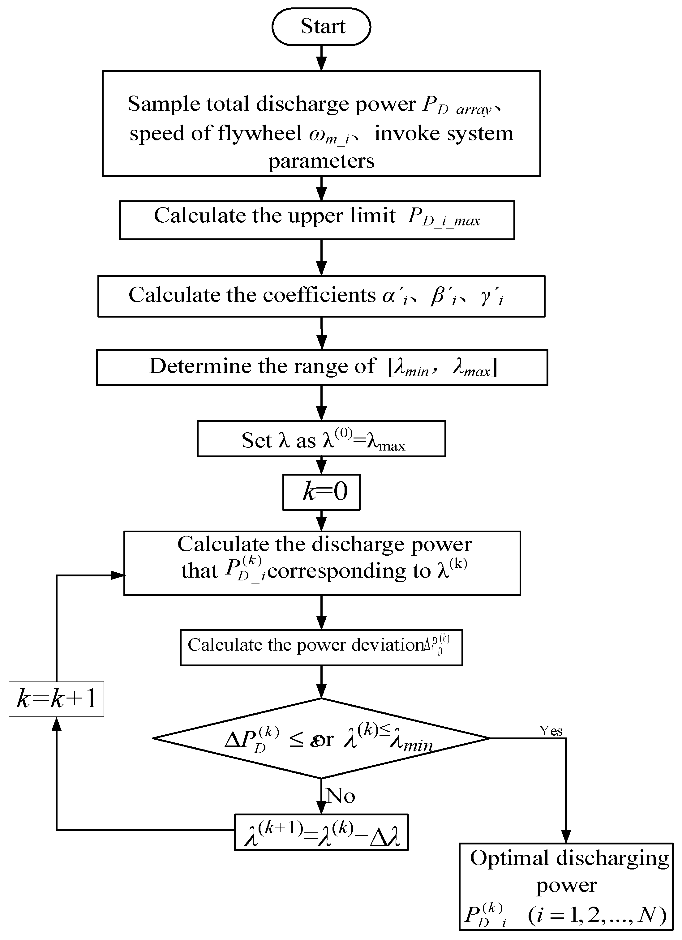
4.3. Research of the Discharging Control Method for the FAESS

The discharging power distribution of the system can be presented as follows. There are the equality constraints:
i = 1 N P D _ i = P D _ a r r a y ,  
and the objective function
P l o s s _ t o t = i = 1 N P l o s s _ i ( P D _ i )
is the minimum.
P l o s s _ i ( P D _ i ) = a i P 2 D _ i + β i P D _ i + γ i represents the loss characteristics of each FESU during discharge. At the same time, the discharging power of each unit P D _ i should satisfy Equation (69).
When the minimum discharging loss of the system is calculated by EIP, a LaGrange function should firstly be constructed according to Objectives (70) and (71).
L = p l o s s _ t o t λ ( i = 1 N P D _ i P D _ a r r a y )
where λ is the LaGrange multiplier.
The necessary conditions for LaGrange function L at the extremum are
{ L P D _ i = P l o s s _ t o t P D _ i λ = 0      ( i = 1 , 2 , , N ) i = 1 N P D _ i P D _ a r r a y = 0 .  
Since the charging loss P l o s s _ i ( P D _ i ) of each unit is only the function that relates to the discharging power P D _ i of each unit,
P l o s s _ t o t P D _ i = d P l o s s _ i ( P D _ i ) d P D _ i = 2 α i P D _ i + β i = λ i      ( i = 1 , 2 , , N )
where λ i represents the incremental rate of consumption of each FESU.
Equation (73) can be rewritten as
{ 2 α i P D _ i + β i = λ      ( i = 1 , 2 , , N ) i = 1 N P D _ i P D _ a r r a y = 0 .  
There are N + 1 equations and N + 1 variables in (75), which means the P D _ i solved by (75) is the value of the distributed discharging power with the minimum loss.
When the discharging power of FESU i based on EIP is lower than the lower limit or higher than the upper limit, the discharging power of the unit will be zero or P D _ i _ m a x . Then, the other FESUs will be distributed as the residual discharging power.

4.4. Implementation Scheme of Discharging Control for the FAESS

After the calculation of distributed power value corresponding to the minimum loss based on the EIP, the directive discharging order will be sent to each bottom controller to realize the discharging control coordination of each FESU, as shown in Figure 13. The main steps are as follows:
(1) The directive value of the total charging power P * a r r a y and the rotating speed of each flywheel ω m _ i are sampled, and systematic parameters are invoked.
(2) The upper limit of discharging power calculated to prevent overcharging and overcurrent of FESU, P O C h _ i _ m a x and P O C u r _ i _ m a x .
(3) The upper discharging limit of each FESU, P D _ i _ m a x , is determined.
(4) The coefficients, α i , β i , and γ i are calculated using the quadratic equation of the discharging loss of FESU P l o s s _ i ( P D _ i ) .
(5) The minimum and maximum values of the incremental ratio of the discharging consumption of each FESU λ i are calculated using
{ λ i _ m i n = β i λ i _ m a x = = 2 α i P D _ i _ m a x + β i      ( i = 1 , 2 , , N ) .  
(6) The minimum and maximum values of the incremental ratio of public consumption of FAESS are determined:
{ λ m i n = min ( λ 1 _ m i n , λ 2 _ m i n , , λ N _ m i n ) λ m a x = max ( λ 1 _ m a x , λ 2 _ m a x , , λ N _ m a x ) .  
(7) The incremental ratio of public consumption is set as λ ( 0 ) = λ m a x .
(8) The charging power P D _ i ( 0 ) corresponding to λ ( 0 ) is calculated using
P D _ i ( 0 ) = λ ( 0 ) β i 2 α i      ( i = 1 , 2 , , N ) .  
If P D _ i ( 0 ) is over the limit, then the limit value is used.
(9) The deviation between sum of discharging power and the total discharging power P D _ a r r a y corresponding to λ ( 0 ) is calculated using
Δ P D ( 0 ) = i = 1 N P D _ i ( 0 ) P D _ a r r a y .  
(10) Verification of whether the power deviation will satisfy the permitted range is carried out using
Δ P D ( 0 ) ε .  
If (80) is satisfied, then P D _ i ( 0 ) is the value of the distributed discharging power with the minimum loss, and P i is given the value of P D _ i ( 0 ) as the directive value of the charging power of FESU.
(11) If (80) is not satisfied, and λ ( 0 ) > λ m i n , then
λ ( 1 ) > λ ( 0 ) Δ λ .
The iterative computations will start again from step (8) until the power deviation satisfies the permitted range or the incremental ratio of public consumption is lower than or equal to λ m i n .
The discharging coordination control program with EIP is shown in Figure 14.

5. Simulation and Experimental Verification

Examples are analyzed to verify the effectiveness of the charging–discharging control strategy for FAESS based on EIP. The IGBT parameters used in the converters of the standardized FESU are shown in Table 1. The parameters of the permanent magnet synchronous motor and flywheel are shown in Table 2. The effective value of the grid voltage is 270 V, the frequency is 50 Hz, and the DC bus voltage of converter U d c is 500 V.
According to Table 1 and Table 2, the loss constants of the standardized FESU can be calculated as shown in Table 3.
The rated power of the standardized FESU is P r a t e d   =   40   kW ; the maximum q-axis current is i q m a x   =   99   A ; the flywheel rotating speed range is [5000 rpm, 10,000 rpm], the upper speed limit is n m a x   =   10 , 000   rpm , and the lower speed limit is n m i n   =   5000   rpm . The time interval of the power distribution is Δ T = 1   s .

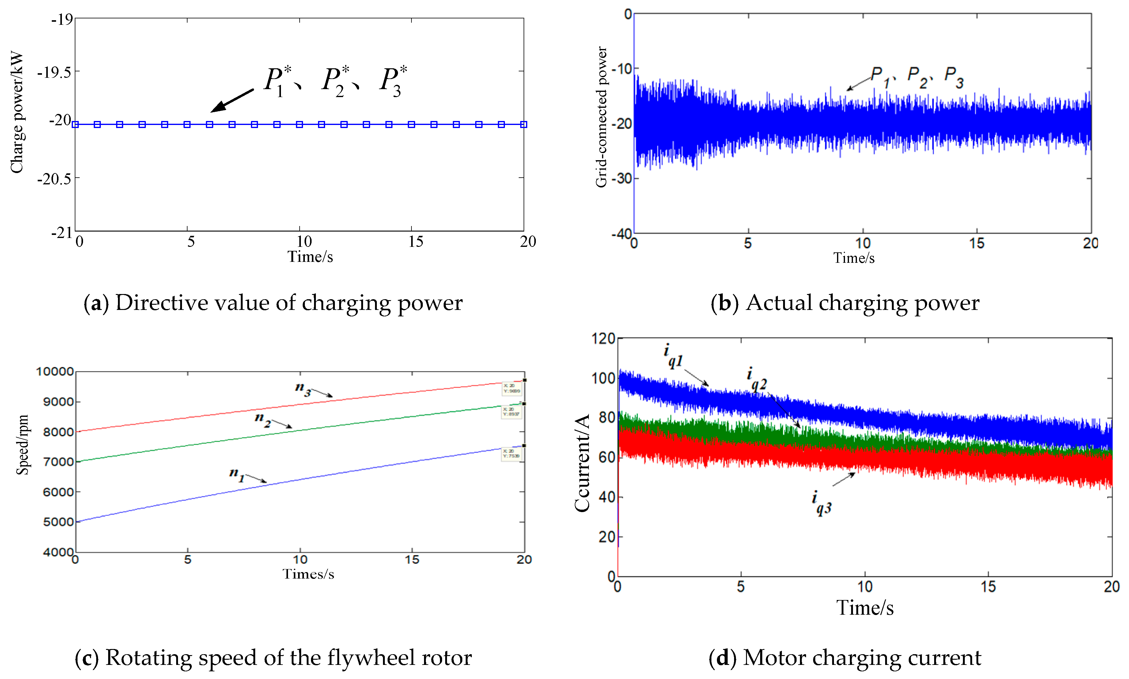
5.1. Charging Example Analysis of FAESS

The FAESS that contains three standardized FESUs is used as an example. A simulation analysis is conducted on three strategies: Equal distribution, distribution by chargeable energy, and distribution by the EIP. The initial rotating speeds of each FESU are n 1 =   5000   rpm , n 1 =   7000   rpm , and n 1 =   8000   rpm , respectively. The speed limits are all n m a x =   10 , 000   rpm . The total charging power is P C _ a r r a y = 60   kW .
(1) The results of charging power distributed by equal distribution
With equal distribution, the directive values of the charging power, the actual charging power, the rotating speed of the flywheel rotor, and the q-axis current distribution are as shown in Figure 15a–d.
According to Figure 15a,b, the directive values of charging power of the three units are all equal to −20 kW. The actual charging powers of the three units are also around −20 kW, which corresponds to the charging directive value. According to Figure 15d, the absolute values of the q-axis currents of the three motors are gradually decreasing, because the charging power is constant and the rotating speed of each motor is increasing. Therefore, the torque of each motor is gradually decreasing, and so is the absolute value of the q-axis current. In addition, as shown in Figure 15c, the rotating speeds of the three flywheels increase from 5000, 7000, and 8000 rpm to 7539, 8937, and 9699 rpm, respectively. After calculation, the total kinetic energy increment is 1049.3   kJ , and the total energy loss is 150.7   kJ .
(2) The results of power charging by chargeable energy distribution
For the chargeable energy distribution, the directive value of the charging power, the actual charging power, the rotating speed of the flywheel rotor, and the q-axis current distribution are as shown in Figure 16a–d.
As shown in Figure 16a,b, the lower the rotating speed is, the larger the chargeable energy of the FESU is and the greater the absolute value of the assigned directive value of charging power is. The charging power of the three units can follow the directive value. According to Figure 16d, when the q-axis current of the first flywheel motor exceeds its maximum value (99 A), overcurrent occurs. In addition, as shown in Figure 16c, the rotating speeds of the three flywheels increase from 5000, 7000, and 8000 rpm to 8250, 8805, and 9119 rpm, respectively. Therefore, the total kinetic energy increment is 1026.3   kJ , and the total energy loss is 173.7   kJ .
(3) The results of power charging distributed by the EIP
With optimal distribution by the EIP, the directive value of the charging power, the actual charging power, the rotating speed of the flywheel rotor, and the q-axis current distribution are as shown in Figure 17a–d.
As shown in Figure 17a, the directive charging value undergoes a larger change when the EIP is used. The absolute value of the directive charging value of the third unit begins to descend and approaches zero, and the absolute values of the directive charging values of the other two start ascending. As shown in Figure 17c, at 18 s, the rotating speed of the third flywheel reaches the upper limit. In terms of the constraints of the EIP, the charging power of the third flywheel is automatically limited. Since the total charging power is fixed, it will only be distributed between the first and second units. Thus, the absolute values of the directive charging values of the two FESUs begin to increase.
According to Figure 17d, the actual charging power of the three units can follow the directive value of the power charging. As seen in Figure 17c,d, there is no over-charging or over-discharging in any of the three FESUs.
In addition, as shown in Figure 17c, the rotating speeds of all three units increase from 5000, 7000, and 8000 rpm to 6797, 9214, and 10,000 rpm, respectively. The total kinetic energy increment is 1052.9   kJ , and the total energy loss is 147.1   kJ .
The calculation above shows that when the charging power is distributed by equal distribution, chargeable energy, and EIP, the total energy loss of the FAESS is 150.7   kJ , 173.7   kJ and 147.1   kJ , respectively. A comparison of these three distribution methods is shown in Figure 18.
According to Figure 18, when the charging power is distributed by EIP, the total energy loss of the FAESS is at the minimum; the loss can be lowered by 15.3% and 2.4% compared with distribution by chargeable energy and equal distribution, respectively. It can be seen from the above simulation analysis results that power charging distribution using the EIP can not only decrease loss, but also avoid overcharging and overcurrent. The simulation results verify the effectiveness of this charging control strategy.

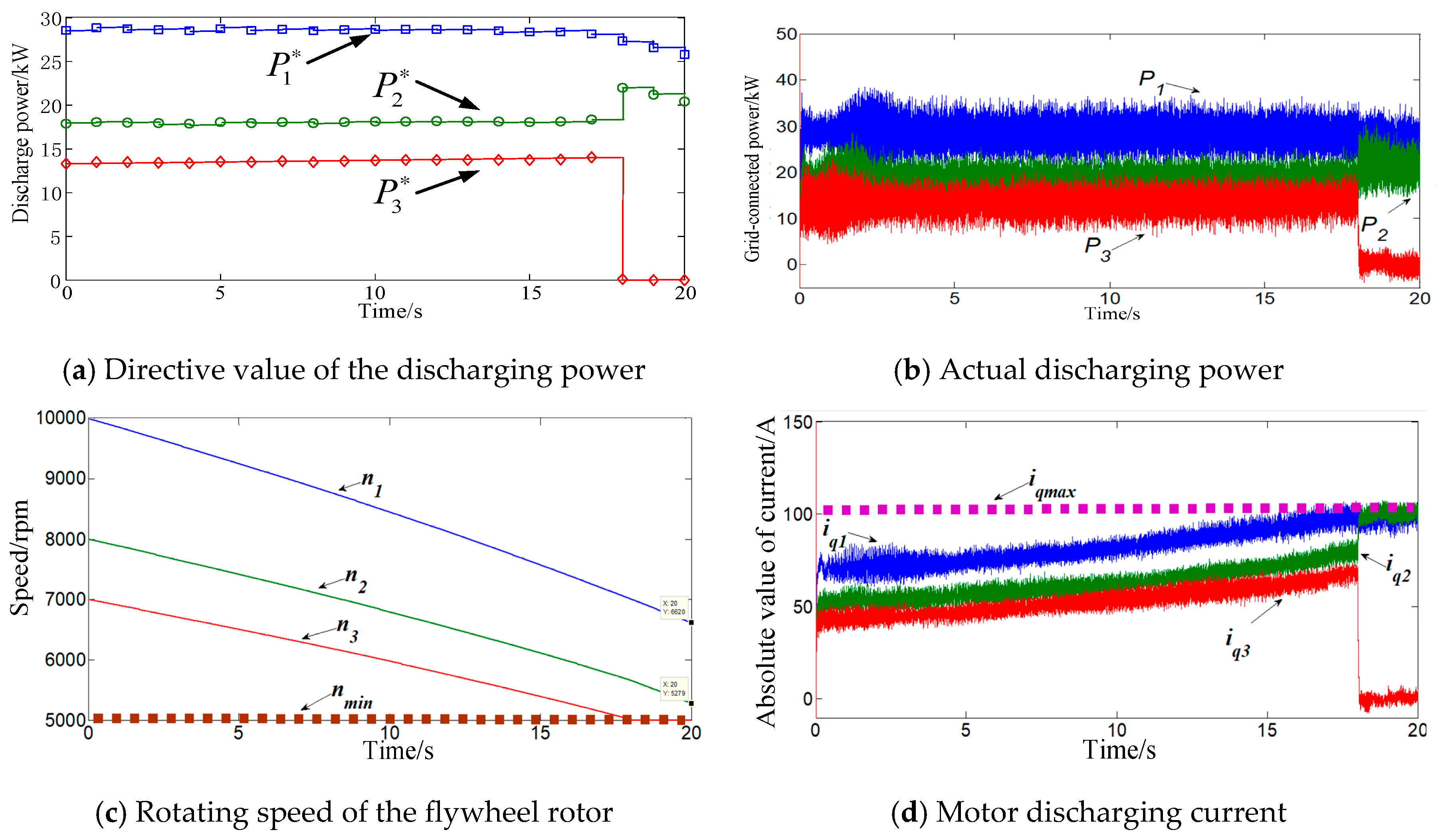
5.2. FAESS Discharging Example

Four strategies—equal distribution, distribution by rotating speed, distribution by residual energy, and distribution by EIP—are simulated. The FAESS that contains three standardized FESUs is again used as an example. The initial rotating speeds of each FESU are n 1 =   10 , 000   rpm , n 2 =   8000   rpm , and n 3 =   7000   rpm , respectively. The lower limit of the rotating speed is n m i n =   5000   rpm and the total discharging power is P D _ a r r a y =   60   kW .
(1) The results of discharging power distributed by equal distribution
With equal distribution, the directive value of discharging power, the actual discharging power, the rotating speed of the flywheel rotor, and the absolute value of the q-axis current distribution are as shown in Figure 19a–d.
According to Figure 19a,b, the directive values of the discharging powers of the three units are equal to 20 kW. The actual discharging powers of the three units are also around 20 kW, which corresponds to the discharging directive value. According to Figure 19d, the absolute values of q-axis currents of the three motors gradually increase, because the discharging power is constant and the rotating speed of each motor is decreasing. Therefore, the torque of each motor gradually increases, as does the absolute value of the q-axis current. When the q-axis currents of the second and third motors exceed the maximum value of 99 A, overcurrent occurs.
In addition, as shown in Figure 19c, the rotating speeds of the three flywheels are lowered from 10 , 000   rpm , 8000   rpm , and 7000   rpm to 7666   rpm , 4931   rpm , and 3079   rpm , respectively. When the speeds of the second and third flywheels are lower than the lower limit, overcharging occurs. The total kinetic energy decrement is 1362.1   kJ , and the total energy loss is 162.1   kJ .
(2) The results of discharging power distributed by the rotating speed
When the discharging power is distributed by the rotating speed, the directive value of the discharging power, the actual discharging power, the rotating speed of the flywheel rotor, and the absolute value of the q-axis current distribution are as shown in Figure 20a–d.
According to Figure 20a,b, the higher the rotating speed, the larger the directive value of discharging power. The actual powers of the three units can follow the directive value of discharging power. As seen in Figure 20d, the q-axis currents of three motors are basically the same.
In addition, as shown in Figure 20c, the rotating speeds of the three flywheels are lowered from 10 , 000   rpm , 8000   rpm , and 7000   rpm to 7072   rpm , 5114   rpm , and 4123   rpm , respectively. When the speed of the third flywheel is lower than the lower limit of 5000 rpm, over-discharging occurs. It is calculated that the total kinetic energy decrement is 1355.3   kJ , and the total energy loss is 155.3   kJ .
(3) The results of discharging power distributed by residual energy
According to Figure 21a,b, the FESU with more residual energy will be distributed with more discharging power. The actual discharging powers of the three units follow the directive value. According to Figure 21d, when the absolute value of the q-axis current of the first motor exceeds the maximum value of 99 A, overcurrent occurs.
In addition, as shown in Figure 21c, the rotating speeds of the three flywheels are lowered from 10 , 000   rpm , 8000   rpm , and 7000   rpm to 5960   rpm , 5530   rpm , and 5329   rpm , respectively. The total kinetic energy decrement is 1340.2   kJ , and the total energy loss is 140.2   kJ .
(4) The results of discharging power distributed by the EIP
When the discharging power is distributed by the EIP, the directive value of the discharging power, the actual discharging power, the rotating speed of the flywheel rotor, and the absolute value of the q-axis current distribution are as shown in Figure 22a–d.
According to Figure 22, at 18 s, the value of the discharging power distributed by the EIP undergoes a large change, and the directive value of the third unit becomes zero. According to Figure 22c, at 18 s, the rotating speed of the third unit reaches the lowest limit. With the constraint for preventing over-discharging in the distribution strategy based on the EIP, the discharging power of the third unit is automatically limited to zero.
According to Figure 22b, the actual discharging powers of the three FESUs can follow the directive value of the discharging power. As seen in Figure 22c,d, there is no over-discharging and overcurrent in any of the three FESUs.
As shown in Figure 22c, the rotating speeds of the three flywheels are lowered from 10 , 000   rpm , 8000   rpm , and 7000   rpm to 6620   rpm , 5279   rpm , and 5004   rpm , respectively. The total kinetic energy decrement is 1315.0   kJ , and the total energy loss is 138.7   kJ .
The above simulation analysis shows that when the discharging power is distributed by equal distribution, rotating speed, residual energy, and the EIP, the total energy loss of the FAESS is 162.1   kJ , 155.3   kJ , 140.2   kJ , and 138.7   kJ , respectively. A comparison of these four distribution methods is shown in Figure 23.
According to Figure 23, when the discharging power is distributed by the EIP, the total discharging energy loss of the system is at the minimum. Compared with the loss of the average distribution, the rotating speed distribution, and the residual energy distribution, the energy loss of can be reduced by 14.4%, 10.7%, and 1.1%, respectively, when the EIP is used. It can be seen from the above simulation analysis that the discharging power distribution based on the EIP can not only decrease the loss, but also avoid over-discharging and overcurrent.
The simulation results verify the effectiveness of the charging–discharging control strategy of FAESS based on the EIP.

6. Conclusions

In this paper, the charging–discharging control strategy for the FAESS is studied in-depth. Firstly, the power loss problem of the FESU during the charging and discharging operation is studied. The results show that the power loss is directly related to power charging–discharging. Based on a relevant theoretical analysis, this paper establishes an objective function of the FAESS with the minimum total power loss as the optimization target. Based on the EIP, it also proposes the constraints of overcharging, over-discharging, and overcurrent. Secondly, a specific implementation scheme for the charging–discharging control strategy for the FAESS based on EIP is proposed. Finally, the charging power distribution strategies (equal distribution, distribution by chargeable energy, distribution by the EIP) are analyzed and compared with examples. In addition, the discharging power distribution strategies (equal distribution, distribution by rotating speed, distribution by residual energy, distribution by the EIP) are analyzed and compared with examples. The results show that the control effect of the charging–discharging control strategy of the FAESS based on the EIP is better than the other control strategies.

Author Contributions

Conceptualization, C.S. and L.Z.; Methodology, C.S.; Software, C.S.; Validation, C.S. and X.T.; Formal Analysis, C.S.; Investigation, T.Z.; Data Curation, C.S. and T.W.; Writing—Original Draft Preparation, C.S.; Writing—Review & Editing, T.W.; Supervision, X.T.; Project Administration, T.W.

Funding

This research was funded by the National Key Research and Development Program of China (2016YFB0900400), the Strategic Priority Research Program of Chinese Academy of Sciences (XDA01020304) and Key Research and Development Program of Hebei Province (19214504D).

Conflicts of Interest

The authors declare no conflict of interest.

References

  1. Chengshan, W.; Zhen, W.; Peng, L. Research on Key Technologies of Microgrid. Trans. China Electrotech. 2014, 29, 1–12. [Google Scholar]
  2. Zheng, Z.; Rongxiang, Z.; Shengqing, T. An Overview on Advanced Grid-connected Inverters Used for Decentralized Renewable Energy resources. Proc. CSEE 2013, 33, 1–12. [Google Scholar]
  3. Tang, X.; Wenjun, L.; Zhou, L. Flywheel Array Energy Storage System. Energy Storage Sci. Technol. 2013, 2, 208–221. [Google Scholar]
  4. Amrouche, S.O.; Rekioua, D.; Rekioua, T. Overview of Energy Storage in Renewable Energy System. Int. J. Hydrog. Energy 2016, 41, 20914–20927. [Google Scholar] [CrossRef]
  5. Mousavi, S.M.G.; Faraji, F.; Majazi, A. A Comprehensive Review of Flywheel Energy Storage System Technology. Renew. Sustain. Energy Rev. 2017, 67, 477–490. [Google Scholar] [CrossRef]
  6. Arani, A.A.K.; Karami, H.G.; Harehpetian, G.B. Review of Flywheel Energy Storage Systems Structures and Applications in Power System and Microgrids. Renew. Sustain. Energy Rev. 2017, 69, 9–18. [Google Scholar] [CrossRef]
  7. Wang, L.; Du, X.; Song, Y. Coordinated Control of Flywheel Energy Storage Matrix System for Wind Farm. Power Syst. Technol. 2013, 37, 3406–3412. [Google Scholar]
  8. Mrugowskyh, H.; Cordt, H.; Sihler, C. Investigation of the Stability of a 600 MJ Energy Storage System Based on Paralleled Flywheel Generators; Electrical Energy Storage Systems Applications and Technologies EESAT: San Francisco, CA, USA, 2002. [Google Scholar]
  9. Huang, Y.; Jiang, X.; Qiu, A. Discharging Control Schemes for Flywheels in Parallel Configuration. Micromotors 2008, 41, 20–24. [Google Scholar]
  10. Zhu, J.; Wang, T. Research of Novel Dynamic Voltage Restorer Based on Flywheel Energy Storage System. Electron. Des. Eng. 2010, 18, 158–161. [Google Scholar]
  11. Cao, Q.; Song, Y.D.; Guerrero, J.M. Coordinated Control for Flywheel Energy Storage Matrix Systems for Wind Farm Based on Charging Ratio Consensus Algorithms. IEEE Trans. Smart Grid. 2016, 7, 1259–1267. [Google Scholar] [CrossRef]
  12. Wang, D.; Sun, Z.; Chen, Y.; Li, S.; Zhao, S.; Wen, H. Application of Array 1MW Flywheel Energy Storage System in Rail Transit. Energy Storage Sci. Technol. 2018, 7, 841–846. [Google Scholar]
  13. Saravia, H.S.; Painemal, H.P.; Mauricio, J.M. Flywheel Energy Storage Mode, Control and Location for Improving Stability: The Chilean Case. IEEE Trans. Power Syst. 2017, 32, 3111–3119. [Google Scholar] [CrossRef]
  14. Guo, W.; Zhang, J.; Li, C.; Su, H. Control Method of Flywheel Energy Storage Array for Grid-connected Wind-storage Microgrid. Energy Storage Sci. Technol. 2018, 7, 810–814. [Google Scholar]
  15. Zhao, J.; Zhang, J.; Song, Z. Distributed Coordinated Control Strategy Based on Flywheel Energy Storage Array System. J. North China Electr. Power Univ. 2018, 45, 28–34. [Google Scholar]
  16. Nemsi, S.; Belfedhal, S.; Makhloufi, S. Parallel Operation of Flywheel Energy Storage System in a Microgrid Using Droop Control. In Proceedings of the International Conference on Wind Energy and Applications in Algeria, Algiers, Algeria, 6–7 November 2018; pp. 1–6. [Google Scholar]
Figure 1. Energy conversion during flywheel charging.
Energies 12 02844 g001
Figure 2. Energy conversion during flywheel discharge.
Energies 12 02844 g002
Figure 3. Structure of the flywheel energy storage unit (FESU).
Energies 12 02844 g003
Figure 4. Equivalent steady state circuit of iron loss resistance.
Energies 12 02844 g004
Figure 5. Energy flowing in the FESU during charging.
Energies 12 02844 g005
Figure 6. Energy flowing in the FESU during discharge.
Energies 12 02844 g006
Figure 7. Prevention of overcharging.
Energies 12 02844 g007
Figure 8. Prevention of overcurrent during charging.
Energies 12 02844 g008
Figure 9. Implementation scheme of the charging coordination control of the flywheel array energy storage system (FAESS).
Energies 12 02844 g009
Figure 10. Flow sheet of charging coordination control based on the equal incremental principle (EIP).
Energies 12 02844 g010
Figure 11. Prevention of over-discharging.
Energies 12 02844 g011
Figure 12. Prevention of overcurrent during discharging.
Energies 12 02844 g012
Figure 13. Implementation of coordination control of discharging.
Energies 12 02844 g013
Figure 14. Flow sheet of discharging coordination control based on the equal incremental principle.
Energies 12 02844 g014
Figure 15. Simulation waveforms of power charging by equal distribution.
Energies 12 02844 g015
Figure 16. Simulation waveforms of power charging distributed by chargeable energy.
Energies 12 02844 g016
Figure 17. Simulation waveforms of power charging distributed by the EIP.
Energies 12 02844 g017
Figure 18. Comparison of the total charging loss.
Energies 12 02844 g018
Figure 19. Simulation waveforms of discharging power distributed by equal distribution.
Energies 12 02844 g019
Figure 20. Simulation waveforms of discharging power distributed by the rotating speed.
Energies 12 02844 g020
Figure 21. Simulation waveforms of discharging power distributed by residual energy.
Energies 12 02844 g021aEnergies 12 02844 g021b
Figure 22. Simulation waveforms of the discharging power distributed by the EIP.
Energies 12 02844 g022
Figure 23. Comparison of total discharge loss.
Energies 12 02844 g023
Table 1. Insulated gate bipolar transistor (IGBT) parameter of the converter.
IGBT On Energy, Eon_test51 mJ IGBT Off Energy, Eoff_test45.5 mJ
Diode on Energy, Erec_test32.5 mJSwitching Frequency, fsw6000 Hz
Test Voltage, Vtest900 VTest Current, Itest225 A
VT01.14 VVD01.1925 V
RCE0.0036 ohm RD0.0027 ohm
Table 2. Parameters of the Flywheel of the Permanent Magnet Synchronous Motor.
Number of Pole-pairs, p2Kc0.11 ohm/rpm
Stator Resistance, Rs0.097 ΩExcitation flux linkage, Ψf0.1286 Wb
D-axis inductance, Ld1.435 mHq-axis inductance, Lq2.085 mH
Viscous friction coefficient, B0.0035 Nm/(rad/s)Flywheel rotating inertia, J2.063 kg m2
Table 3. Total Loss Constant of the FESU.
b5.8733c0.004725
d0.0178f4.321 × 10−8
g0.1455h0.3858
k12.4829 × 10−5k2−3.79 × 10⁻⁶
k30.094457l−0.9822

