1. Introduction
Subjective evaluation of a vehicle by test drivers is an important part of the final assessment of vehicle performance. In most cases, these evaluations are done on test tracks or under real world conditions like on the Autobahn. The feedback from drivers is the input for the fine tuning of vehicle dynamics [
1,
2]. The impact of aerodynamics also contributes to the ratings from the test drivers on ride quality and directional stability [
3]. Most of the research available that is related to aerodynamics and its influence on vehicle dynamics is on the impact of cross-wind/gusts stability and vehicle response [
4,
5,
6,
7,
8,
9]. In these examples, the field of straight line drivability without external influences such as cross-winds/gusts are not considered. A vehicle showing low standard in straight line drivability at high speed is seldom unstable in a strict mathematical way, rather it is uncomfortable or ’nervous’ to drive. According to Proton et al. [
10], drivability is defined as the smoothness of vehicle operation under all driving conditions. It determines the vehicle’s ability to behave according to customers requirements. In this case, poor straight line drivability rating at high speed by the test driver can be due to poor lane keeping ability, feel of disturbance in the form of lateral acceleration or yaw acceleration or need of subtle but frequent, steering input from the driver.
Research relating objective measurements to subjective judgements is found in few papers. Klause et al. [
11] studied objective evaluation of subjective judgement on secondary ride comfort; i.e, vibrations > 4 Hz and handling. Ten cars of different categories such a sports and luxury cars were studied. Hence, the results of handling characteristics were scattered. The results could only point out the potential of either handling or steering improvement for a given car. Their methodology did not explain on how to commonly formulate the objective rating factor for any vehicle. Chandrasekaran et al. [
12] focused on comparing objective and subjective drivability on a compact SUV. They used neural networks with the help of the AVL drive software to determine objective drivability ratings. This software aids in measuring physical quantities such as vehicle speeds and accelerations via sensors and interfaces. The driving conditions are recognized with fuzzy logic. The investigation at constant speed was one among ten maneuvers of the driving cycle. The driving environment for constant speed maneuver such as, whether it is a straight road, existence of external disturbances such as road unevenness was not explained. Moreover, it is difficult to give formula or interpret relationships resulting from a neural network between physical quantity to the objective drivability.
Strandemar et al. [
13,
14], used ISO 2631 to show that transient disturbances play important role in subjective evaluation. They pointed out that the basic evaluation tool used in ISO 2631 is the Weighted acceleration RMS value which decreases the contribution of transient nature. ISO 2631, Evaluation of Human Exposure to Whole-body Exposure [
11] is commonly used for determining the ride quality of a vehicle under a condition consisting of a consistent disturbance pattern such as road roughness. It agrees with subjective rating provided the vibrations are stationary in nature. An alternative method called the ride diagram, introduced by Strandemar et al. [
15] was used to visualize vehicle excitations with transient events separated from the stationary signal. A signal is characterized as a stationary signal when, at any two time instance, any signal value is equally probable of happening with respect to any other signal value irrespective of the distance between these signal values. On the other-hand, a transient signal show presence of sudden jumps in an otherwise stationary signal. Their investigation was on vertical ride comfort and no further research on remaining variables such as lateral acceleration, pitch or yaw rate was carried out. Also the subjective tests were done on different test drivers using a motion simulator behaving as a real truck under different suspension characteristics. Tests on a real on-road test will tend to have more uncertainties than a controlled environment such as a simulator.
For this study, a sedan vehicle is considered with on-road tests done on a test track with two straight sections, each long enough to capture the influence of the aerodynamic devices added to the model. The flow around the vehicle is altered to create asymmetric flow patterns intended to result in undesired aerodynamic forces and moments on the vehicle. The purpose of these aerodynamic devices is to develop substandard driving quality at high speeds during straight line drive. Three configurations are considered in this study; an inverted wing, an inverted wing with an asymmetric flat plate and an asymmetric air curtain attached to the diffuser. All the three configurations have the primary intention to increase the lift of the vehicle. These configurations are paired with and without side-kicks. The side-kicks are additional aerodynamic devices used to create a defined flow separation line in the rear side of the vehicle intending to stabilize the rear wake. Comparison of the subjective judgement from a trained test driver are done between the pair of configurations. Combining any of the other aerodynamic devices with side-kicks results in an improved drivability. Various sensors are used to record the vehicle behaviour. This study aims to find a relationship between these measurements and subjective judgements. Objective measures would be very useful to support virtual verification/evaluation on earlier stages of vehicle development.
2. Experimental Set-Up
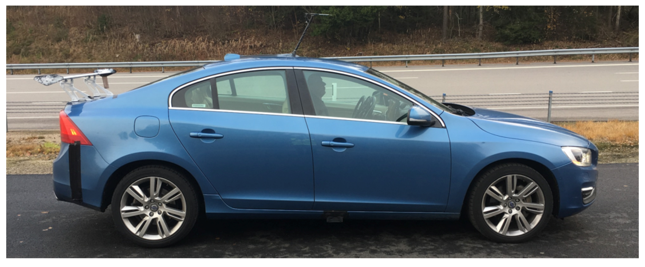
In this study, the test object is a mid-size sedan, shown in
Figure 1. The car is front wheel driven giving a more forward load distribution than the four wheel driven version. This enhances the sensitivity in the rear due to lower traction on the rear tires. The instrumentation used, the configurations studied and the test track and test procedure will be discussed next.
2.1. Instrumentation
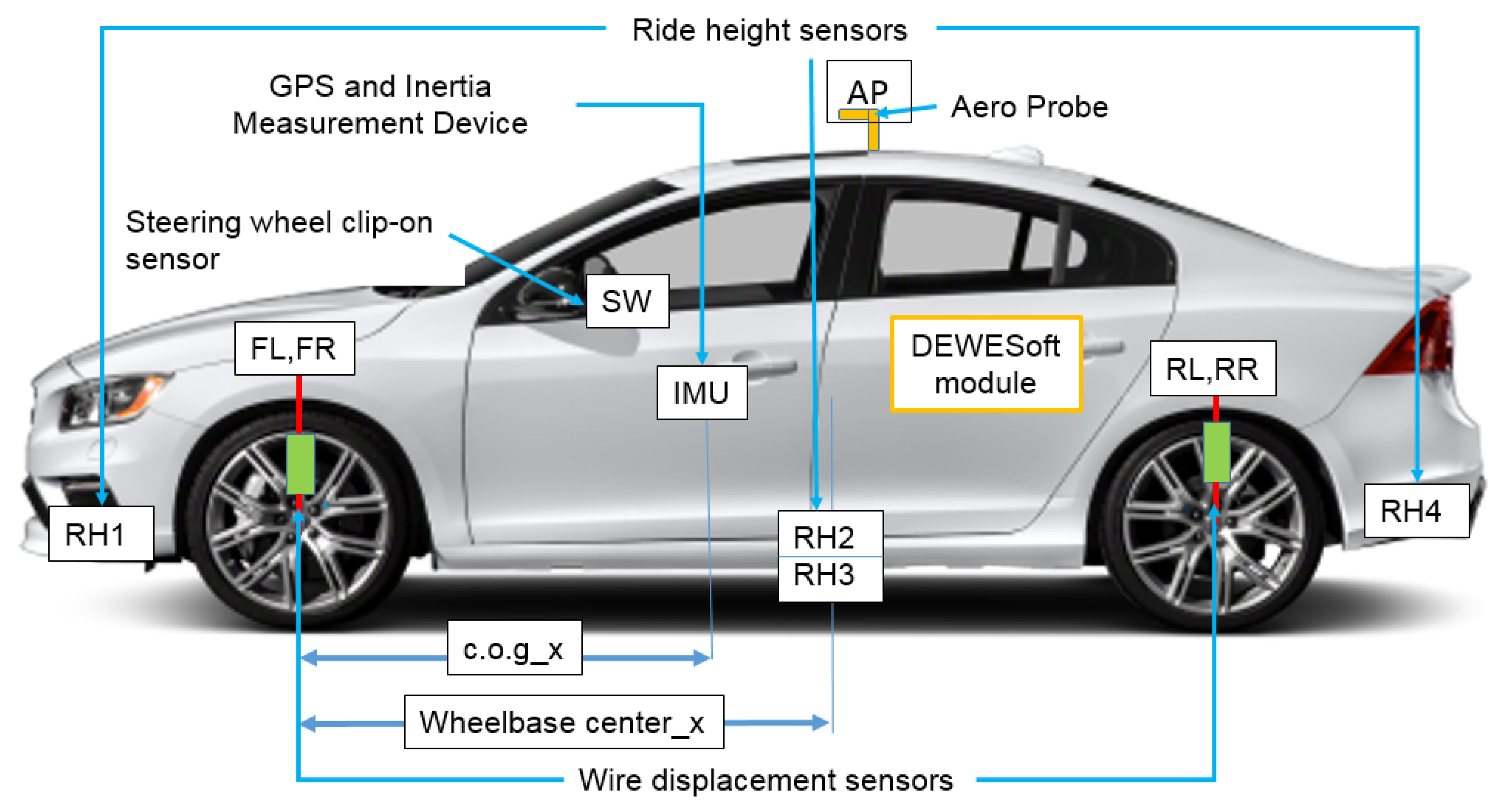
In order to capture the vehicle behaviour, different variables are recorded with the help of sensors. As shown in
Figure 2, the added sensors are as listed below:
Steering Wheel clip-on sensor (SW): This sensor measures the steering angle and the steering torque. The steering effort sensor, part of the device, is fastened on the steering wheel like an auxiliary steering wheel. the other part is attached to the windshield with the help of vacuum and is used to get the angular position. A belt drives the angular position sensor which is connected to the steering effort sensor. Analog outputs are produced from the two sensors using an analog converter [
16]. The effort sensor has an uncertainty of
deg. However, the reference positioning of the angular position sensor is not accurate and therefore neither are absolute values. SW is apt for comparing the change in steering behaviour between different conditions.
Aeroprobe and pressure sensors (AP): The head wind condition plays an important role in the aerodynamics of the vehicle as a result it is important to track the head wind angles during the test. The aeroprobes have 7 ports at the tip measuring the respective pressures. These pressure values can later be used to calculate the slip angle, roll angle and angle of attack of the head wind. They have a range of
and an accuracy of
. The aeroprobe is placed over the roof of the test object at a vertical height of 360 mm from the roof, in line with Reference [
17]. In the XY plane, it is placed in the intersection of the lines bisecting the wheelbase and track width. The disturbances created by cylindrical aeroprobe holder in the form of vortex shedding are minimized by using helical strakes. The pressure sensors are placed inside a small box on the roof in between the aeroprobe holder and the antenna with minimal interference to the flow.
Ride height sensors (RH1, RH2, RH3, RH4): Attaching aerodynamic devices results in change of ride height of the test vehicle. There are four sensors attached to the test object. One placed inside the front bumper, another inside the rear bumper making the it flush with the exterior surface and remaining two sensors are placed to the sides at the middle of the wheel base. They are attached to the stiff body structure to minimize the influence of dynamic flexing of the body. Measurement of uncertainty for the sensor is .
Inertia Measurement Unit (IMU): It is also placed in the center of gravity of the vehicle except for the z coordinate (due to structural hindrances). However the IMU can translate the readings of any reference point one inputs, irrespective of the position of IMU itself. Although the measuring acceleration closest to driver gives the best correlation between objective and subjective measure, from previous studies the acceleration measurements vary a lot between test runs and test drivers as a result the repeatability is quite low [
11]. In addition, the region of interest is the quality of vehicle drivability which is associated with rigid body and chassis dynamics; that is, frequency <4 Hz. This falls in to the primary ride comfort category. The IMU is positioned, as suggested by ISO 2631 [
18], to the vehicle structure in the interest for chassis vibrations and behaviour. GPS is integrated to this system with the positioning of antennas as recommended by DEWESoft [
19].
Draw-wire displacement sensors (FL, FR, RL, RR): The displacement of suspensions shows aerodynamic and road influence on the vehicle. Four sensors are co-aligned with the spring of each wheel, each able to measure a displacement of with an uncertainty below .
CAN signal: Signals from the vehicle’s built-in sensors are also recorded. The steering wheel angle data considered in this research during post-processing and plots is recorded from the CAN bus. The accuracy of these sensors are .
Dewesoft Module: All the sensors are conected to the data acqusation system called Sirius Dewesoft. Dewesoft X software is used for data acquisition and some post processing.
2.2. Aerodynamic Configurations
As mentioned, the tests involved creating intentional substandard drivability in order to observe the driver’s response. One way to reduce the straight line driving standards is to reduce the traction between tires and road surface. With less traction between road and tires, the test object becomes more sensitive to undesired forces or moments. Paper by Jeff Howell et al. [
20] provides a better understanding on relation between lift over lateral aerodynamic characteristics for passenger cars, providing motivation towards modifying the rear of the vehicle. The chosen aerodynamic devices increase lift forces of the test object to favour this need. Referring to Human Perception Theory by Heeger [
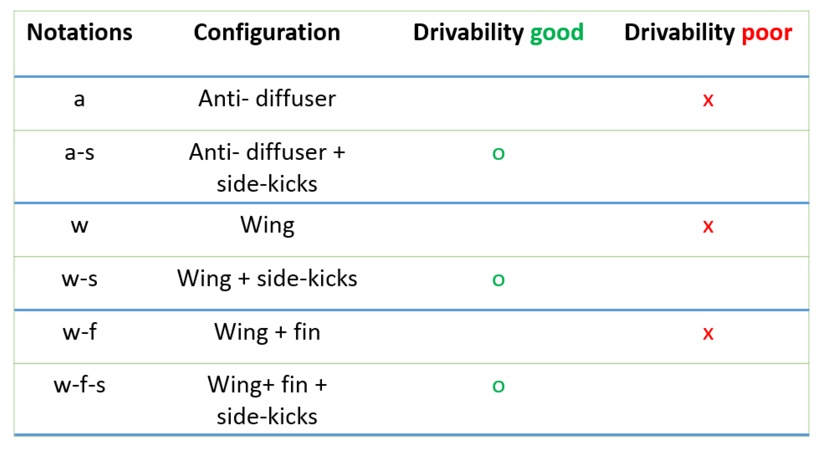
21], stimulus of different intensities are created with different aerodynamic devices and their combinations and the test driver is asked to respond if he senses it or not. This subjectively establishes sensory absolute thresholds of the test driver. The absolute threshold is the minimum intensity required to be detected by the test driver. After test driving different combinations of a number of aerodynamic devices, three paired configurations are selected for this study. The chosen aerodynamic devices for these configurations are:
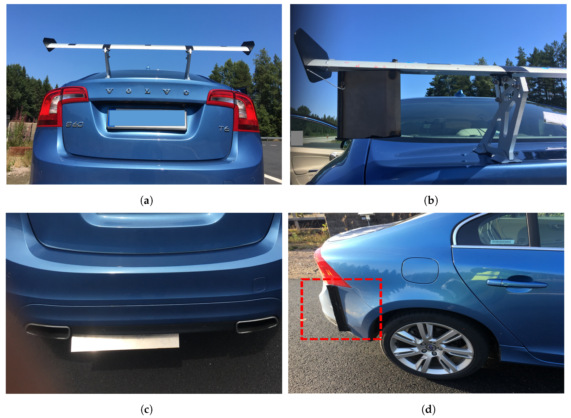
Inverted Wing [w]: The wing is attached inverted, like on an aircraft, to the boot-lid of the vehicle, as shown in
Figure 3a, in such a way that it generates more lift in the rear. The angle of attack of the wing is
. Several test runs are done with tufts on the wing to adjust to the maximum possible angle of attack before stall. The behaviour of the tufts is viewed using cameras attached to the winglet.
Wing with fin [w-f]: The second device is a fin is placed
to the flow upstream on the left side of the inverted wing, as shown
Figure 3b. With the addition of a fin on only one side, the wing is expected to experience asymmetric force and moment.
Anti-diffuser [a]:
Figure 3c shows the anti diffuser, which is an asymmetric air curtain placed under the rear bumper. It is positioned to guide the flow downwards and partially restrict the flow along the diffuser region. The resulting asymmetric downwash is expected to affect the vehicle base wake behaviour thus creating non-uniform and periodic forces and moments on the vehicle. This device is termed anti-diffuser as it acts opposite in functionality to a diffuser. The device is suppose to promote a downwash resulting in rear lift.
Side-kicks [s]: Side-kicks are additional aerodynamic devices shaped as separation edges on both sides of the rear bumper, as shown in
Figure 3d. They also have a slight spike to create an outwash while separating the flow at the defined locations. The objective of the side-kicks is to repair the negative effects induced by the three configurations, i.e, wing [w], wing with fin [w-f] and anti-diffuser [a].
2.3. Test Track and Test Procedure
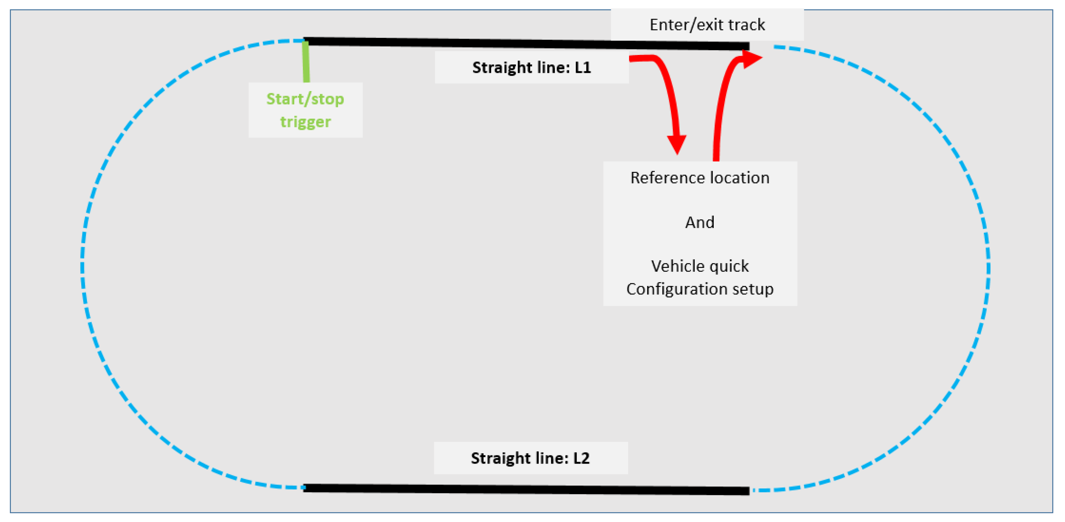
The tests are performed at the Volvo Cars Hällered Proving Ground. The test track used for this study is an oval track with two straight lines of 1.1 km, as sketched in
Figure 4. Only measurements along the two straight lines are considered.
The test begins with the test object at the reference location where the sensors are tared. By doing so, the measured values are the difference from the reference position. The test object is first run at high speed to heat the tires to a temperature that remains consistent during high speed drives. The tire pressure is periodically monitored during the tests to ensure its consistency and safety After that it is set to desired configuration and parked at the reference position where a tare is performed. The test object is then driven around the track and the driver is assigned to keep the test object in a straight line. As soon as it passes the first straight line L1, provided the speed is the intended speed and consistent, the Dewesoft Module starts data acquisition. The recording of the data is triggered using coordinates at the beginning of L1 and stops after three full laps. As soon as the recording is complete the test object returns to the reference location for setting up the next configuration and the sensors are tared. This process is repeated for all planned configurations. Throughout the test, the test driver is unaware of the configurations and what to expect from them especially while attaching and detaching the side-kicks, hence providing an unbiased judgement. The tests are done for four different speeds: 140, 200, 230 and 250 km/h. Differences in vehicle behaviour are only observed at speeds of 230 and 250 km/h. Hence, these two speeds are considered in the analysis. Six readings are considered for each speed, three for straight line L1 and three for straight line L2 for speeds 230 and 250 km/h. These speeds are measured using GPS with an accuracy of . The speed is kept constant using cruise control which an accuracy of at 230 and 250 km/h. The average wind speed and direction are received from the traffic control over each test run. The test is done only when the wind speed is below 2 m/s thus minimizing the head angle. During trial runs the subjective judgements are done by three test drivers for all three configurations pairs. In addition, the first author is always present in the passenger seat in all the tests. The tests with recorded data which are presented in the paper are only for one driver. The drivers are not explained about the influences or the set-ups of the aerodynamic devices attached on the test vehicle. As a result, this can be considered as a blind test.
3. Drivability Analysis Methods
To understand vehicle response to an excitation, such as steering angle, the transfer function from steering angle to lateral acceleration or yaw velocity is commonly used. All aerodynamic excitations and responses are small in this test, so transfer function becomes sensitive to sensor errors. The investigated transfer functions do not show that the response is dependent on the input. The input and output coherence between the signals in the test data is fluctuating over each frequency and is weak on average over the desired frequency spectrum, So, no credible transfer functions can be found from the kind of tests done.
In an attempt to relate the subjective feel of the test driver to measurable quantities, a few basic variables are considered: lateral acceleration
, yaw velocity
, steering angle
and steering torque
. Roll and heave rates also contribute to subjective judgment especially in cases such as cross-wind and high speed lane change maneuvers. In this study, straight line drive, their influence is negligible hence they are not further discussed. While
and
are feed-backs of vehicle response to aerodynamic disturbances,
and
can be either the vehicle response or the driver’s response or combination of both to aerodynamic disturbances. The data received from the test consists of three laps and four speeds as mentioned in
Section 2. Only the two straight lines, named L1 and L2, are considered in the analysis.
3.1. Mean Value Vector Plots Method
Six mean values are considered for each speed, three for L1 and three for L2 for speeds 230 and 250 km/h. The mean is calculated for a quantity
x separately for each speed according to the equation:
where
N is the number of samples. Vector lines connecting the values of the desired quantities of the configurations without side-kicks to the corresponding configurations with side-kicks are referred as vector plots.
Here, plotting mean values of against and connecting configurations without side-kicks to the corresponding configurations with side-kicks give respective vector plots. These vector plots show the trend of vehicle handling for each configuration pair.
3.2. Standard Deviation Vector Plots Method
The number of independent samples,
m, of each signal is found using auto-correlation function [
22]. This function calculates the correlation between
and
, where lag
. According to Box et al. [
23] the auto-correlation for
k is
where,
is the sample variance of the time series.
where
T is the effective sample. The variance of the signals are:
The mean uncertainty with a coverage factor of 2, which corresponds to a coverage probability of approximately 95%, is:
3.3. Ride Diagram Method
The mean and variance show an average vehicle response to different configurations but lacks the ability when it comes to understanding the presence of transient behavior. The ride diagram uses a filter to separate the transient behaviour from the remaining signal. The method for ride diagram is done in three steps, defined by Strandemar et al. [
24]. The signal is divided into segments at the sign changes of the signal derivatives as shown in Equation (
6).
Thus the
kth segment will be expressed as:
where
and
is total number of peaks. The peak-to-peak value of
kth segment is:
The segments can now be categorized as transient or stationary according to:
where
and
is the number of segments.
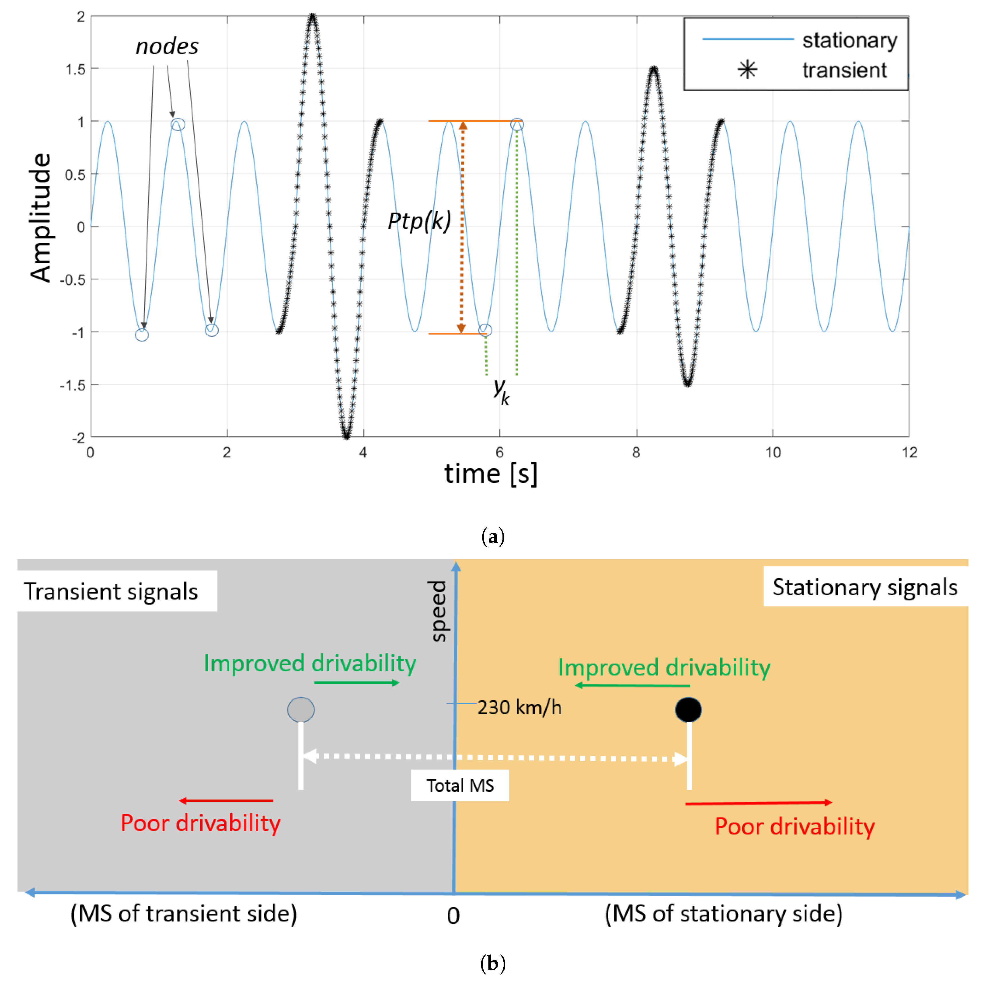
Figure 5a shows an example of a random signal. As referred in Strandemar et al. [
24],
is the limit of transients also know as the signals energy equivalent amplitude. The Mean Squared Values (MS) of transient and stationary (remaining) signals are related as shown in Equation (
10).
For a given situation
Figure 5b shows a general idea of reading the ride diagram with respect to drivability standards.
4. Discussion and Results
Three configurations that give subjective substandard drivability are selected. Side-kicks are then added to improve drivability. The subjective rating of the tests are shown in chart
Figure 6.
The different configurations gives the following behaviours:
The inverted wing gives low frequency sway, believe to be excited from the rear end of the test object.
The inverted wing with fin shows similar behaviour as just the inverted wing but in addition there is a slight leftward yaw.
The anti-diffuser shows a more high frequency yaw behavior compared to the other configurations.
The use of side-kicks improves drive quality and notably dampens the above mentioned behaviours of the respective configurations.
4.1. Limitations
In this work the significance of subjective judgement is based on statistics. Higher the number of test drivers and test runs, the better the significance of the judgement. However, time taken for testing all these configurations by each driver along with the desired weather conditions are some limitations to be considered. In this test three test drivers are used for subjective evaluation during trial runs and the recorded data presented is of only one test driver. This collection of subjective evaluation along with six runs each should be statistically significant.
Despite major changes to the test object with the intention to increase the lift, the subjective feel for disturbances is still subtle. No alarming instability issue could be sensed by the test drivers which was the prior intention. The relative effect; i.e, comparison with all configurations against each other, was difficult due to time constrains. In addition, when the behaviour is subtle, it is difficult to keep subjective judgement in mind of all configuration tests and rate them against each other. Mind saturation and exhaustion plays a significant role in subjective rating. Since the feel is subtle, the energy and concentration required for the evaluation is significant.
The presence of uncertainty for some measurements is also a challenge which is solved using statistical support as later discussed in
Section 4.3.
4.2. Analysis
The data received from the test sensors are filtered with low pass filter with a 20 Hz cutoff frequency and the feedback from the test drivers is expected to be due to effects below 2 Hz. This falls in the primary ride quality which is related to vehicle chassis behaviour, as mention in
Section 3.
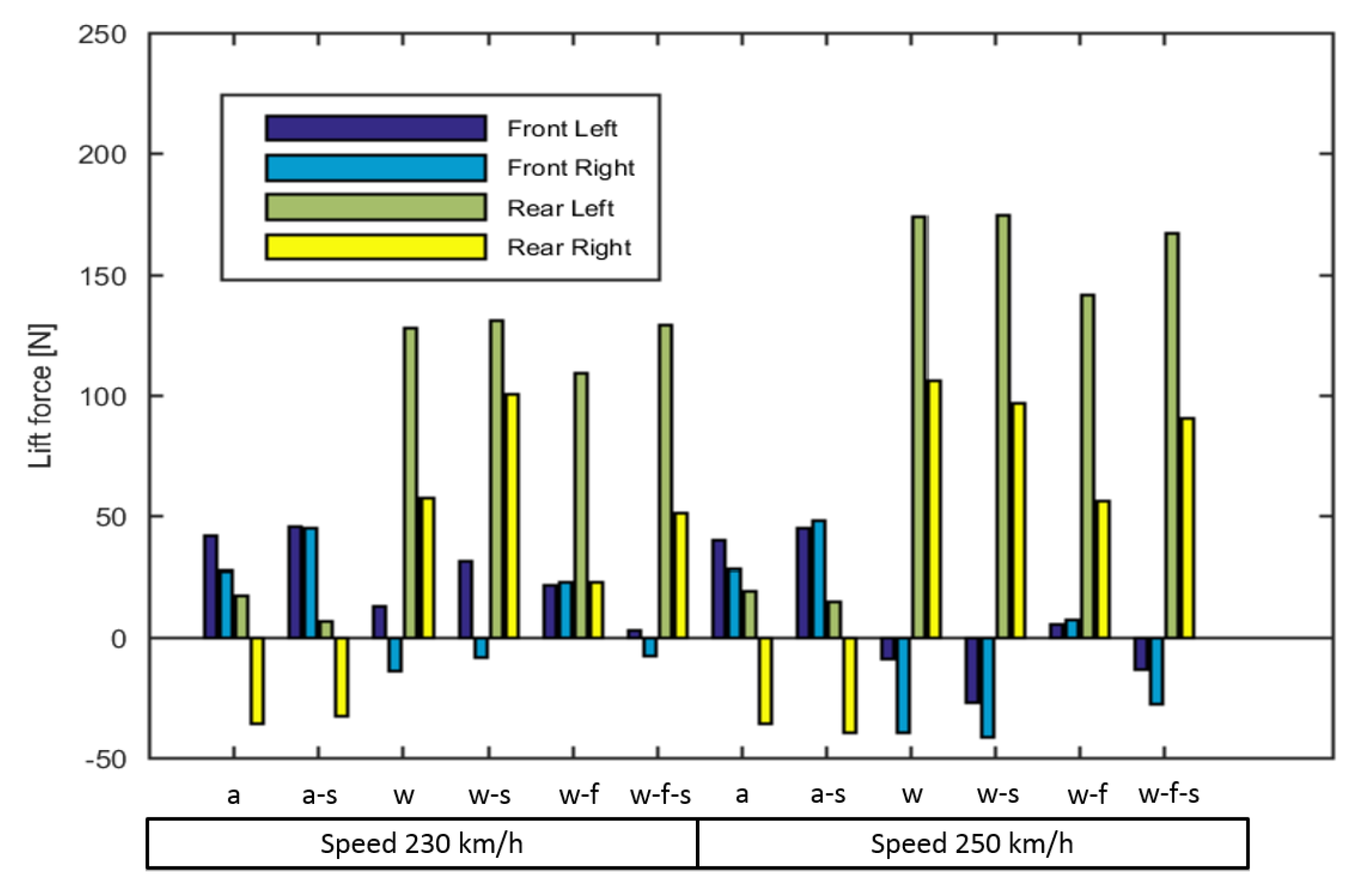
Wire displacement sensors are used to determine the lift forces of all the configurations which are compared with the reference test object, that is, the test object without any configurations. The RMS of the change in lift forces on each wheel for each configuration compared to the reference test object is shown in
Figure 7. It is interesting to observe that the configuration with anti-diffuser (a and a-s) creates less lift distribution on rear right wheel compared to the reference. The rear right suspension receives a lower lift force where the anti-diffuser is not restricting the flow along the diffuser and the rear left has higher lift where the anti-diffuser restricts the flow along the diffuser. The configurations with anti-diffuser provide the lowest lift forces of all the configurations independent of speed. For the wing (w and w-s) and wing with fin (w-f and w-f-s) configurations, the increase in speed from 230 to 250 km/h results in higher rear lift. As a result the load is being redistributed more to the front of the test object. This causes the front suspension to compress and the test object to pitch down. When comparing the configuration pairs in
Figure 7, it is hard to make any conclusive statement on the side-kicks’ contribution to lift. The asymmetric suspension expansion between rear left and right is also notable in this bar graph. This could be due to a difference in unsprung weight.
4.2.1. Comparison Using Mean Values
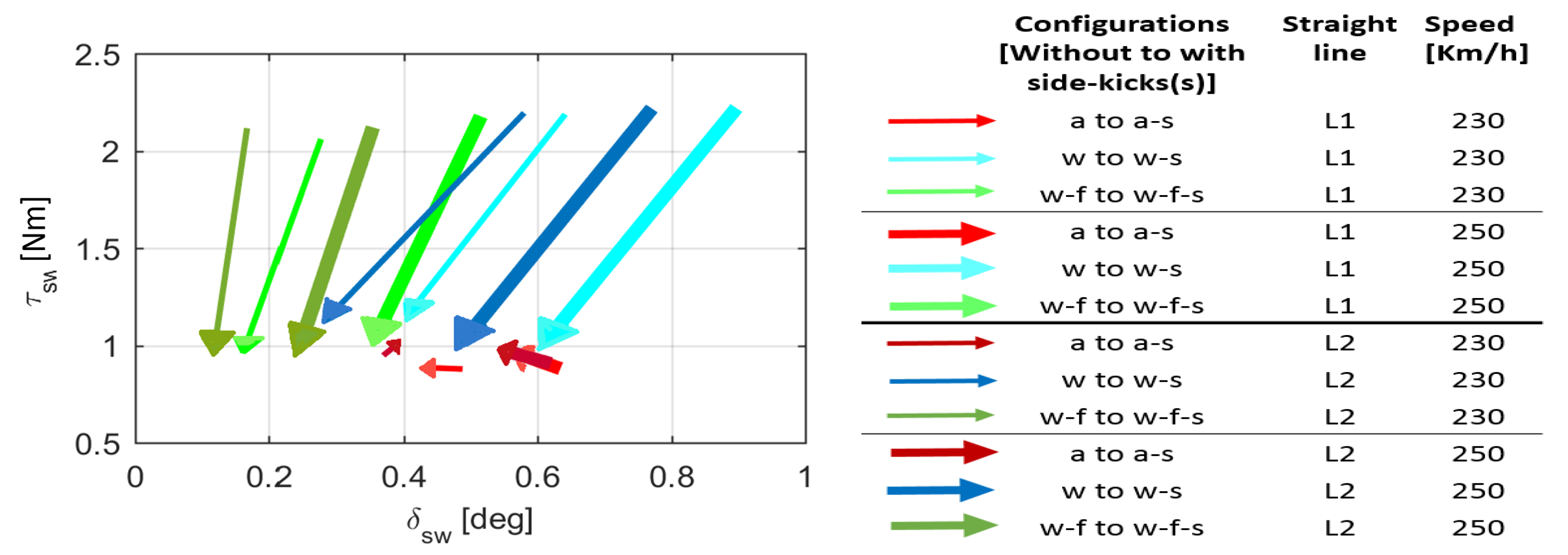
Figure 8 depicts the effect on mean steering behaviour of the test object with vector plot of steering angle
in x axis and steering torque
in y axis. Since the car follows a straight line, the mean values of lateral acceleration
and yaw velocity
are close to zero as the lateral displacement an rotation of the test object from start to end of a straight line are negligible. In the case of
and
, the mean value depicts the excess averaged steering input required by the driver in response to exterior disturbances while keeping the test object following the straight line. It is intuitive to interpret that low
and
together with lower need for
and
response shows the characteristics of good drivability. This characteristics is shown by arrow pointing towards the origin.
Figure 8 shows the improvement in drivability for configurations with side-kicks as they require lower
and
compared to ones without side-kicks. Although the subjective judgement of the configuration with anti-diffuser (red arrows) suggests an improvement in drivability due to side-kicks, the results are not as clear as for the other configurations (wing and wing with fin). The vector plots suggests that unlike the other configurations the driver requires similar mean steering response within the pair. Except for the configuration pair with anti-diffuser, the steering characteristics have marked their importance when it comes to high speed straight line drive subjective judgement.
4.2.2. Comparison Using Standard Deviations
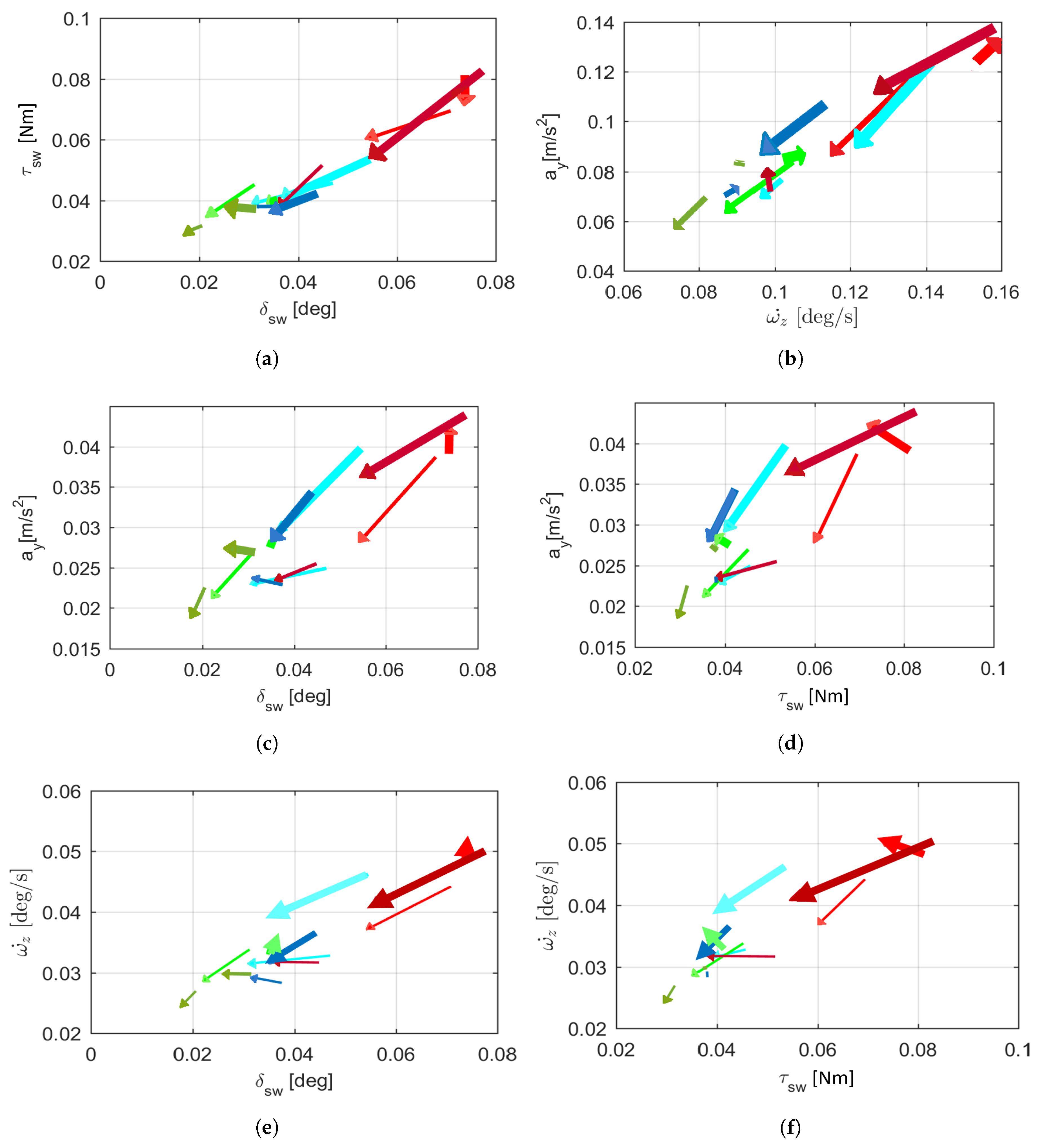
The standard deviation comparison is of major interest as it shows unsteady behaviours of a vehicle. The vector plots in
Figure 9 show the change in standard deviation for all configurations with and without side-kicks. The configuration pair with anti-diffuser (a to a-s) shows a notable behaviour change between with and without side-kicks, unlike in the mean vector plots. This suggests that side-kicks dampen the unsteady vehicle behaviour resulting in better driving on a straight line. Similar behaviour is seen in the configurations with wing and wing with fin. It is interesting to note that in
Figure 9 the configuration with anti-diffuser at 250 km/h have only steering torque
improvement with side-kicks at straight line L1. Similarly, the wing with fin configuration (w-f to w-f-s) has no influences with respect to vehicle response, i.e, lateral acceleration
and yaw velocity
at 250 km/h. However, in general the vector plot pattern of configurations without side-kicks to with side-kicks is towards the origin of the graph, showing a reduction in magnitude of all the variables investigated. This is inline with the subjective judgement of an improved drivability.
4.2.3. Comparison Using Ride Diagram
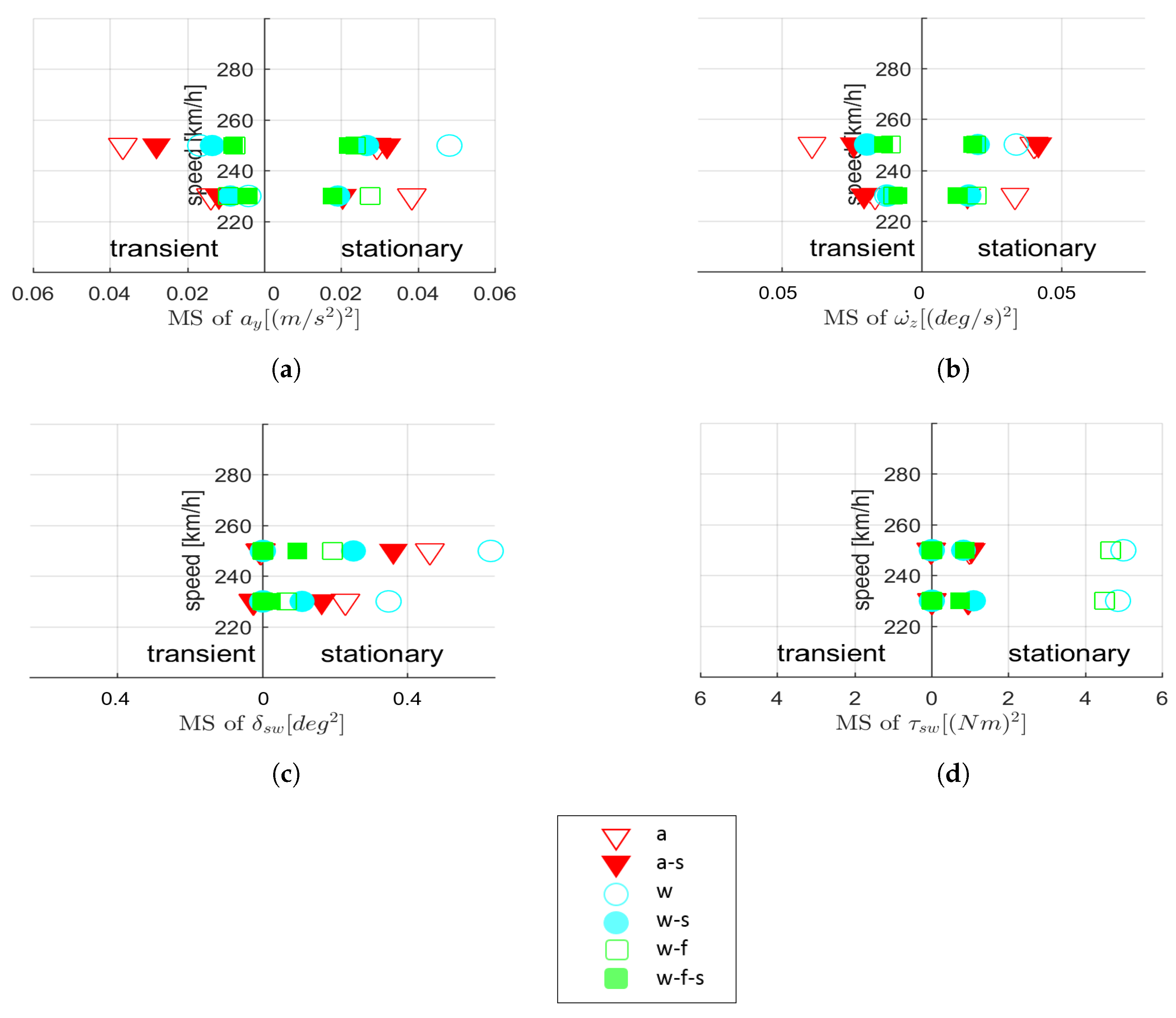
Figure 10 shows ride diagrams of all configurations using all four variables considered. The graph plots the MS values of the transient part of the signal to the left and the MS values of remaining (stationary) signals to the right. Unfilled markers represent respective configurations without side-kicks and filled markers represent configurations with side-kicks. The sum of MS values of transient and stationary gives the total MS value of the signal.
Figure 10a,b show that the contribution of transient nature is larger in the configuration with anti-diffuser compared to other configurations. The steering characteristics, as seen in
Figure 10c,d show a larger contribution on the stationary side, especially for wing and wing with fin configurations and the transient contribution is negligible in comparison. This shows the inability to respond to unknown transient behaviours. This is clearer while comparing the steering characteristic,
, of all the configurations in
Figure 10d where the wing and wing with fin configurations have significant
difference between with side-kicks and without side-kicks.
Figure 10 showing the simple representation of how the ride diagram is looked into, portraits that the further the MS value is from the origin on the x axis, the lower the standard of drivabilty. The ride diagrams interpreted this way agree with subjective judgement of all configurations.
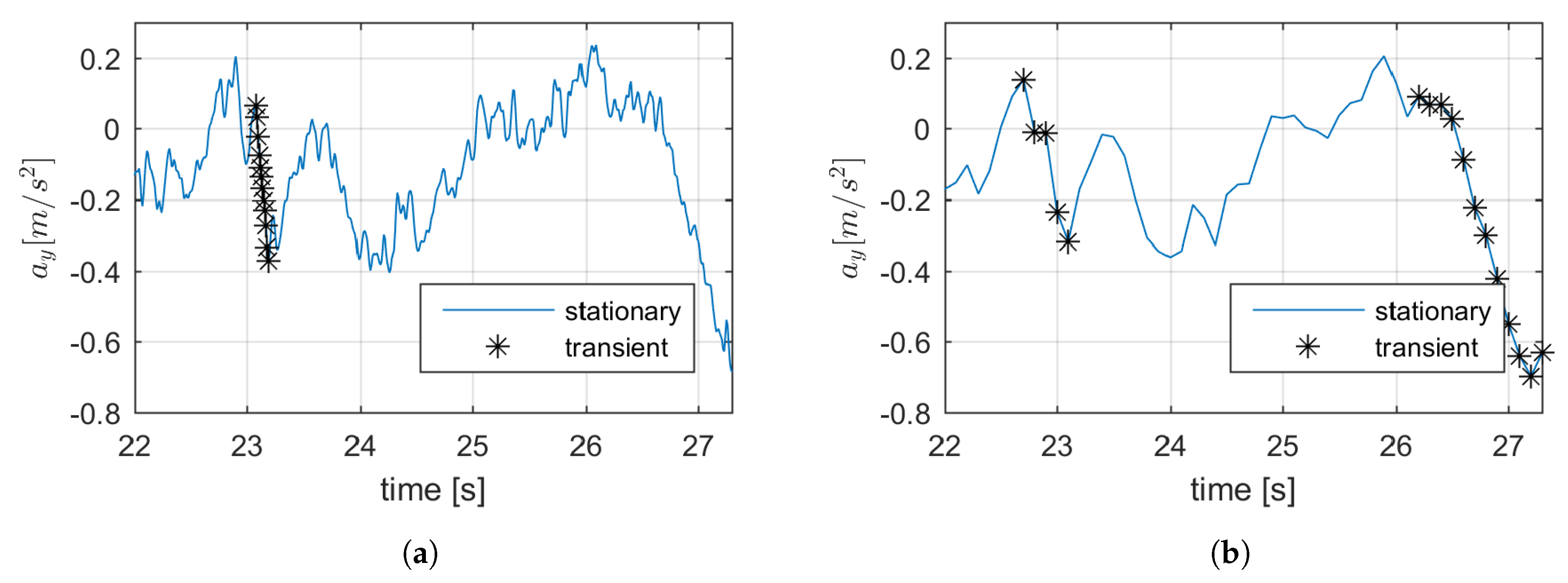
This method has some practical issues when the signals have small spikes in them. These spikes can be located in between an otherwise high peak-to-peak value as shown in
Figure 11, as from time 26 to 27 s. As a result while separating the signals with the
criterion, it only checks for the exact peak-to-peak values between these spike as set by the filtering mechanism. So the possibility is high for a peak-to-peak value, which would otherwise be eligible for being filtered as a transient segment, to not be filtered because of spikes. This can be reduced by downsampling the signals but this does not completely eliminate the problem. The method was originaly used by Strandemar et al. [
24] for relatively simple signals for testing in a driving simulator. Hence it needs further development for more realistic signals.
4.3. Statistical Analysis
It has been shown that the use of mean and variance vector plots and Ride diagram matches the driver’s subjective judgment on drive quality. But the measurements fall in the error region of for accelerometers and gyroscope. This brings the certainity of observations from the above plots to a grey area especially for lateral acceleration
and yaw velocity
. This eliminates the possibility of a quantitative analysis. Due to the consistent vector patterns, usually pointing towards the origin, a statistical analysis can support the qualitative evaluation. Cumulative Binomial distribution is used to assess the probability of random creation of such a pattern. The probability of atleast
x successes in
n trials:
In this case the null hypothesis is that there is no difference between the configurations, depending on if they have side-kicks or not and that gives the assumption
. The number of trials
n is twelve. With these values taken into account the binomial distribution of the success of each of the four variables at
n trials are calculated as shown in
Table 1. This shows that the probability for the random vector plots to show similar pattern as that of the results is quite low. In comparison to all the variables considered the probability of such a case in
is the highest with
which is low but still notable. The null hypothesis can be rejected for
,
and
.
5. Conclusions
The objective of this test is to correlate the driver’s subjective judgement of drivability with measurable quantities. In this study several aerodynamic configurations are used to create undesired forces and moments: Inverted wing, inverted wing with fin and anti-diffuser. These configurations are tested in pairs with and without side-kicks. The test driver is asked for a subjective evaluation of the test object at high speed straight line driving with these configurations. The main conclusions of this test are the following:
The configurations with side-kicks show an improvement in straight line drivability compared to the respective ones without side-kicks and it is believed that the reason for this is because of a better defined flow separation with sidekicks. The analysis models presented in this study show a trend that agrees with the subjective judgement of the test driver.
The vector plots of mean and standard deviation point toward the origin. This implies that the vehicle response and steering efforts to aerodynamic disturbances are reduced with side-kicks, depicting the improved subjective assessment of drivability.
The study suggests that smaller standard deviation of steering angle, steering torque, yaw velocity and lateral acceleration gives better subjective assessment of drivability at high speed straight-line driving.
The Ride diagrams show the contribution of transient nature, if any, in these configurations along with the ability to differentiate the pairs on substandard drivability.
The Ride diagram methodology needs to be further developed in order to capture real signals having spikes which deceive the current filtering mechanism in considering potential transient segments as non-transient.
The limitation of the accuracy of the sensors used makes it a qualitative analysis with the help of a statistical assessment. In order to quantify drivability in a robust way, more accurate sensors are needed along with more configurations showing even worse drivability and instability conditions.
Analysis of suspension displacements of all four wheels suggests that the side-kicks achieved improved straight line drivability without notable lift changes within the pair.
The side-kicks can be used as an aerodynamic device for subjective evaluation while comparing different configurations. To accept side-kicks as a production solution, its influence on drag needs to be investigated using computational fluid dynamic simulations or wind tunnel tests.
Author Contributions
Contribution of the authors are as follows: Conceptualization, formal analysis, data curation, investigation and writing—original draft preparation is done by A.K. Methodology is done by A.K. with the support from B.J.H.J. Software: Matlab is used for data analysis by A.K. with the support from E.S. Validation is done by A.K. and E.S. Resources are provided by A.B. and E.S. Writing—review, editing and visualization is done together with S.S., E.S., B.J.H.J. and A.K. Supervision done by S.S., E.S. and A.B. Project administration managed by A.B.
Funding
This research was funded by the Swedish Energy Agency and the Strategic Vehicle Research and Innovation Programme (FFI).
Acknowledgments
The authors would like to thanks Mats Jonasson from Chalmers University for his help and valuable comments. The authors are also very grateful to the Volvo Cars Hällered Proving Ground, mechanics and instrument support. The author is also grateful to Volvo cars and Hällered Proving Ground vehicle test engineers for their contribution.
Conflicts of Interest
The authors declare no conflict of interest. The funders had no role in the design of the study; in the collection, analyses, or interpretation of data; in the writing of the manuscript, or in the decision to publish the results.
Abbreviations
The following abbreviations are used in this manuscript:
| IMU | Inertia Measurement Unit |
| MS | Mean Square Value |
| RMS | Root Mean Square Value |
| CAN | Controller Area Network |
References
- Park, S.J.; Lee, Y.S.; Nahm, Y.E.; Lee, Y.W.; Kim, J.S. Seating Physical Characteristics and Subjective Comfort: Design Considerations; SAE Technical Paper; SAE International: Detroit, MI, USA, 1998. [Google Scholar]
- Qunan, H.; Huiyi, W. Fundamental Study of Jerk: Evaluation of Shift Quality and Ride Comfort; SAE International: Detroit, MI, USA, 2004. [Google Scholar]
- Hucho, W.H.; Warrendale, P.A. Aerodynamics of Road Vehicles, 4th ed.; Butterworth-Heinemann: Oxford, UK, 2013; ISBN 978-0-7506-1267-8. [Google Scholar]
- Huemer, J.; Stickel, T.; Sagan, E.; Schwarz, M.; Wolfgang, A.W. Influence of unsteady aerodynamics on driving dynamics of passenger cars. J. Veh. Syst. Dyn. Int. J. Veh. Mech. Mobil. 2014, 52, 1470–1488. [Google Scholar] [CrossRef]
- Carbonne, L.; Winkler, N.; Efraimsson, G. Use of Full Coupling of Aerodynamics and Vehicle Dynamics for Numerical Simulation of the Crosswind Stability of Ground Vehicles. SAE Int. J. Commer. Veh. 2016, 9, 359–370. [Google Scholar] [CrossRef]
- Forbes, D.; Page, G.; Passmore, M.; Gaylard, A. A Fully Coupled, 6 Degree-of-Freedom, Aerodynamic and Vehicle Handling Crosswind Simulation using the DrivAer Model. SAE Int. J. Passeng. Cars - Mech. Syst. 2016, 9, 710–722. [Google Scholar] [CrossRef]
- Juhlin, M. Directional stability of buses under influence of crosswind gusts. J. Veh. Syst. Dyn. Int. J. Veh. Mech. Mobil. 2007, 46, 827–835. [Google Scholar] [CrossRef]
- Fukagawa, T.; Shimokawa, S.; Itakura, E.; Nakatani, H.; Kitahama, K. Modeling of Transient Aerodynamic Forces based on Crosswind Test. SAE Int. J. Passeng. Cars Mech. Syst. 2016, 9, 572–582. [Google Scholar] [CrossRef]
- Schroeck, D.; Krantz, W.; Widdecke, N.; Wiedemann, J. Unsteady Aerodynamic Properties of a Vehicle Model and their Effect on Driver and Vehicle under Side Wind Conditions. SAE Int. J. Passeng. Cars Mech. Syst. 2011, 4, 108–119. [Google Scholar] [CrossRef]
- Isa, I.Y.A.M.; Abidin, M.A.Z.; Mansor, S. Objective Driveability: Integration of Vehicle Behavior and Subjective Feeling into Objective Assessments. JMES 2014, 6, 782–792. [Google Scholar] [CrossRef]
- Klaus, W.; Hoppermans, J.; Kraaijeveld, R. Objective Evaluation of Subjective Driving Impressions. Soc. Automot. Eng. Jpn. 2008. [Google Scholar]
- Chandrasekaran, K.; Rao, N.; Palraj, S.; Kurella, C.; Lebbai, M.N. Objective Drivability Evaluation on Compact SUV and Comparison with Subjective Drivability. Symp. Int. Automot. Technol. 2017. [Google Scholar] [CrossRef]
- Strandemar, K.; Thorvald, B. The Ride Diagram, A Tool for Analysis of Vehicle Suspension Settings: The Dynamics of Vehicles on Roads and on Tracks. J. Veh. Syst. Dyn. Int. J. Veh. Mech. Mobil. 2006, 44, 913–920. [Google Scholar] [CrossRef]
- Strandemar, K.; Thorvald, B. Driver perception sensitivity to changes in vehicle behavior. Veh. Syst. Dyn. 2004, 272–281. [Google Scholar]
- Strandemar, K.; Thorvald, B. Truck Characterizing Through Ride Diagram: In Vehicle Dynamics and Chassis Developments. Sae Commer. Veh. Eng. Congr. 2004. [Google Scholar] [CrossRef]
- PM Intrumentation. 2017. Available online: https://pm-instrumentation.com/docpdf/Systemes/embarque-volant/PMI-01184-Volant-telemetrique.pdf (accessed on 15 May 2019).
- Oettle, N.R.; Sims-Williams, D.; Dominy, R.; Darlington, C.; Freeman, C.; Tindall, P. The Effects of Unsteady On-Road Flow Conditions on Cabin Noise. SAE Int. J. Passeng. Cars Mech. Syst. 2011, 4, 120–130. [Google Scholar] [CrossRef][Green Version]
- ISO. Mechanical Vibration and Shock: Evaluation of Human Exposure to Whole-Body Vibration. 1997. Available online: https://www.iso.org/standard/7612.html (accessed on 19 May 2019).
- DEWESoft. Documentation on IMU and GPS. 2019. Available online: https://dewesoft.com/products/ interfaces-and-sensors/gps-and-imu-devices (accessed on 20 May 2019).
- Howell, J.P.; Fuller, J.B. A Relationship between Lift and Lateral Aerodynamic Characteristics for Passenger Cars; SAE Technical Paper; SAE International: Detroit, MI, USA, 2010. [Google Scholar]
- Heeger, D. Course Notes for Introduction to Perception. Available online: https://www.coursehero.com/sitemap/schools/17-Stanford-University/courses/2113753-PSYCH30/ (accessed on 12 December 2018).
- Hamilton, J.D. Time Series Analysis, 4th ed.; Princeton University Press: Princeton, NJ, USA, 2013; ISBN 978-0-6910-4289-3. [Google Scholar]
- Box, G.E.P.; Jenkins, G.M.; Reinsel, G.C. Time Series Analysis: Forecasting and Control, 3rd ed.; John Wiley & Sons: New Jersey, NJ, USA, 2008; ISBN 978-1-118-67502-1. [Google Scholar]
- Strandemar, K. On Objective Measures for Ride Comfort Evaluation. Ph.D. Thesis, KTH Royal Institute of Technology, Stockholm, Sweden, 2005. [Google Scholar]
© 2019 by the authors. Licensee MDPI, Basel, Switzerland. This article is an open access article distributed under the terms and conditions of the Creative Commons Attribution (CC BY) license (http://creativecommons.org/licenses/by/4.0/).

 ,
, 


