Assessment for the Age-Of-The-Air and Ventilation Efficiency in Confined Outdoor Spaces through Computational Fluid Dynamics Techniques

Abstract

An experimentally validated numerical method for evaluating the suitability of an urban design with regard to its capacity to provide the optimum air quality for its occupants through the confined outdoor spaces is proposed. Eight possible confined outdoor spaces are defined according to their position with regard to the built elements, laterally delimited by the envelope surfaces of the neighbouring buildings. This work focuses on the definition of a procedure capable of analysing outdoor air change quality according to the age-of-the-air concept. The obtained results show that the confined outdoor spaces that are exposed to the wind action are more predisposed to reduce the mean age-of-the-air that they contain. For the analysed cases, a considerable improvement of up to 78.68% in the air change quality can be obtained by taking into account wind exposure criteria in relation to its shape and urban density, which is classified for this purpose.

1. Introduction

The effect of air change in urban areas consists of the mixing of volumes of air with different hygrothermal characteristics and molecular composition, as well as the pollutant agents contained within. “Clean” air coming from open areas from the neighbouring suburban environment mixes with the urban air [1]. This mix, the product of the particle exchange between polluted air volumes and clean air volumes, generates the air quality renovation, which depends on wind velocity among other factors. With a constant contamination intensity in the cities, the greater the wind velocity is, the greater the air flow incoming to the urban area will be, which expedites the mix [2]. However, the residence time of the clean air inside the urban area is reduced, as is the efficiency of the natural air change process [3].

This ideal flow is only produced under the “piston model”, which is the hypothetical case produced by constant friction on all limiting surfaces of the model and the lack of obstacles that may hinder the natural flow path. Analysis of the different possible circumstances in urban environments will promote the knowledge of their impact degree on air quality.

“Clean” air has been defined as air that features an acceptable pollutant proportion for its use by individuals. Its quality, however, will depend on the constraints of suburban areas surrounding the studied cities. This incoming air to the urban areas will carry external agents to the air’s natural composition (suspended particles, dust, microorganisms, pollen, etc.), although it is considered to all effects to be of higher quality than the air contained in urban areas in steady conditions, which presents a larger quantity of pollutants from industry, combustion processes, etc.

This is due to the rural and suburban areas having their air recycled by the natural processes from the vegetation present in larger numbers in these environments, unlike in urban spaces. In this process of displacement of air particles inside urban spaces, these particles get loaded with pollutants and harmful agents for the human being. The greater the air flow incoming from suburban areas is, the greater the air quality will be, as this mix effect will be occurring in a shorter period of time, reducing the instantaneous concentration of toxic and pollutant agents.

The air flow between buildings through outdoor spaces constricts its quality through the subsequent continuous contamination process. Parameters such as population density, the presence of industry, or traffic significantly influence the air decay process. The situation is caused to a large degree by the demographic increase in population centres which require a considerable number of services which uphold the expected benefits in order to maintain the quality of life of the citizens. However, green areas and a permeable urban plot enable a substantial improvement in outdoor air quality to be consumed by the buildings’ and cities’ users, not just backed by the “clean” air contribution and aerial pollutant neutralisation, but also derived to a large extent from the alteration of the air path coming from suburban areas, that facilitate its renovation process through mixing.

“Outdoor confined urban spaces” refer to those air volumes that, to a larger or lesser extent, are confined between built surfaces and that generate the urban plan, usually open in their upper ends [4], and that allow air particle displacement in a more or less winding way between buildings and other urban elements. Those spaces provide “clean” air to the indoor living spaces and renovate the “polluted” air released by them.

For the current work, the definition of these spaces has been restricted by their position with regard to built elements, laterally delimited by the envelope surfaces of neighbouring buildings and with height rising up to the cornice height of the tallest building in the outdoor space (Figure 1). The set of confined outdoor spaces comprises the “urban profile”. The study of air quality patterns in those spaces orients to the analysis of its behaviour regarding the impact of the cities’ aerodynamical agents over this behaviour. Objectively, the outdoor spaces with a smaller interface with free air will be the outdoor spaces with larger difficulties in air renovation due to their design (Figure 2 and Figure 3).

Ventilation consisting of the intake of outdoor air as a way of diluting harmful particles present in the indoor air of living spaces requires outdoor spaces that guarantee its quality. This is achieved through outdoor spaces sufficiently open to free air, that due to their constructive and geometric conditions promote its exchange and mixing.

The outdoor air in its free movement is affected by multiple variables in rural, suburban, and urban areas which condition its cinematic and dynamic behaviour to be developed inside the cities. Those variables alter its dispersal, modifying the quality of the air between the different outdoor spaces, passageways, and edificatory voids [5,6]. It can be said that the final quality of the air introduced into buildings for their ventilation depends on

• the confluence of air healthiness conditions in its origin (suburban areas);
• pollution, and the type and concentration of contaminants emitted in the urban area;
• path or characteristic route of an amount of air from its entry in the urban area to its exit, including the retention time in indoor spaces; and
• the ability of the urban outdoor spaces that feed the premises to exchange their air with the free air current.

2. Outdoor Air Change Quality and Efficiency

The air change efficiency of the air contained within spaces is defined by the age-of-the-air concept. This concept allows the connection between the path and development of each moving air particle inside a model with the quantity of time it resides within the model. In other words, it enables us to know the retention time of the air particle set [7,8]

This age-of-the-air concept can be used in more complex systems such as outdoor spaces assimilating an urban model to a limited and delimited model such as a large indoor space. The boundary conditions of this space must be known and applied on equal terms as if it was an indoor space, assuming that the air must enter and exit from the model freely but identifying the virtual limits by which this fact is produced.

Experimentation on age-of-the-air in large outdoor spaces is difficult to carry out due to the reduced control and tracking capacity of tracer gas particles in these environments. High discharge flows of tracer gases are required in order for the concentrations to be correctly sampled by the measuring equipment. This type of tests becomes feasible in scaled experiences in which emissions are managed and concentrations are assessed through any of the valid methods pointed out by [9] (Equations (1)–(3)). In the same way, simulation on computational fluid dynamics (CFD) software is today used to assess air quality in outdoor spaces [9,10], assimilating boundary conditions of the simulated tunnel to the boundary conditions of an indoor space:

$${\overline{\tau }}_p=\frac{c}{\dot{m}}$$

(1)

$$Q_{\infty }=\underset{A}{{\displaystyle \int }}{U}_{\infty }dS$$

(2)

$${\overline{\tau }}_p^{\ast }=\frac{{\overline{\tau }}_p·Q_{\infty }}{V}$$

(3)

where: ${\overline{\tau }}_p$ is the local mean age-of-the-air; ${\overline{\tau }}_p^{\ast }$ is the local normalised mean age-of-the-air; $\mathrm{c}$ is the local concentration (kg/kg); $\dot{m}$ is the homogeneous emissions index; $S$ is the Surface normal to the air flow in vectorial components; $Q_{\infty }$ is the air flow passing though the Surface $S$; $U_{\infty }$ is the component air velocity in the free air current ($\approx U_m·\left(\alpha +1\right)$); $V$ is the air volume in the control zone; $U_m$ means profile air velocity; and $\alpha$ is an exponent determined by the exponential equivalent profile of air velocities.

Having said that, the problem of age-of-the-air assessment depends on the analysed urban environment and the boundaries and dependencies considered inside a control volume. Control volume refers to a portion of air that, because of its characteristics or position inside a larger volume, enables a specific analysis. The dimensional characteristics of this type of volume for the analysis of the air behaviour surrounding a solid volume have been defined in preceding research works.

By limiting a greater volume, a virtual volume whose surfaces must satisfy the flow equilibrium criterion from the continuity equation (Equations (4) and (5)) is generated; the inlet flow to the control volume must be equal to the outlet flow. This way, the mean age-of-the-air volume will be considered dependent on the mean age-of-the-air in the areas where the flow is positive (air entering the control volume) and the mean age-of-the-air where the flow is negative (exits the control volume) (Figure 4).

$$Q=Q_i=Q_o$$

(4)

$$Q={\displaystyle \sum }_n{Q}_{in}={\displaystyle \sum }_n{Q}_{on}$$

(5)

Consequently, the air change process efficiency in a determined volume responds according to Equations (6)–(8):

$${\tau }_n=\frac{V}{Q}$$

(6)

$${\tau }_r=2\langle {\overline{\tau }}_p\rangle$$

(7)

$${\xi }^a=\frac{{\tau }_n}{{\tau }_r}\le 1$$

(8)

where $Q$ is the balanced flow of air in the control volume; $Q_i$ and $Q_o$ are air flows at the inlet and the outlet; ${\tau }_n$ is the theoretical age-of-the-air at the outlet; ${\tau }_r$ is the mean age-of-the-air at the outlet (air retention time in the control volume); ${\tau }_p$ is the mean age-of-the-air of the volume; and ${\xi }^a$ is the air change process efficiency [11].

The theoretical age-of-the-air at the outlet will depend on the flow passing through the model, assuming it is under the criterion of the “piston model” (Equations (9)–(11)) in which fluid continuity without the influence of obstacles that generate the creation of vortices or turbulent movements is assumed. The space in which the hypothetical “piston model” is produced can be considered as the ideal case in which the age-of-the-air increases in a lineal progressive manner in its path with a homogeneous age-of-the-air in the outlet surface (Figure 5). That results in the mean age-of-the-air being the average of the ages at the inlet and at the outlet.

The application of this concept over the boundary conditions established for urban models of outdoor air requires a specific study of the attitude of the air under the conditions of the velocity and turbulence profiles as a product of the free flow of air and the action of the wind. Under ideal conditions, the nominal flow rate in a model is dimensioned according to the equivalent flow of the perpendicular projection of the open surfaces of the volume considered on the velocity profile of the global model (Equations (9)–(11)), as a projection of the cross section of the urban model (Figure 6).

$$Q_i=Q_o=\left(y_2-y_1\right)·\left(z_2-z_1\right)·\frac{{{\displaystyle \int }}_{z_1}^{z_2}f\left(u\right)dz}{z_2-z_1}$$

(9)

$$Q_i=Q_o=\left(y_2-y_1\right)·{{\displaystyle \int }}_{z_1}^{z_2}f\left(u\right)dz$$

(10)

$$Q_i=Q_o=\frac{U^{\ast }}{k}·\left(y_2-y_1\right)·\left({\left[z·Ln\left(\frac{1}{z_0}\right)\right]}_{z_1}^{z_2}+{\left[z·Ln\left(z\right)-z\right]}_{z_1}^{z_2}\right)$$

(11)

3. CFD Model Configuration

The model is configured to a scale appropriate to the experimental support validation made at 1/200 scale. The use of scaled models has been widely justified for validations made over field experiences in real environments [12,13,14] and CFD simulation enables the study of the air behaviour over ideal models so as to obtain a global vision of the relationship between the air and the built volumes [13,15,16,17].

Numerical calculation is nowadays a tool capable of simulating the air behaviour in real models, reducing the cost of on-site experimentation and enabling the analysis of multiple variables intervening in the outdoor air change process. It has allowed the affordable study of air behaviour in outdoor spaces based on air turbulence standards simulations.

The studied physical environment will be considered as an ideal fluid at constant temperature without thermal or mechanical influences different from the diffusion or movement promoted by the environment, its characteristics, and the various obstacles that can influence its free movement. This simplification obviates the dynamic impact of a nonisothermal criterion of the surfaces. This criterion would cause the difference of air densities due to its temperature, which would imply a pressure gradient in the model. This gradient would entail air mass displacements beyond the boundary conditions established in this paper.

3.1. Physical and Numerical Principles

The disturbances in the flow path in a turbulent regime [18,19,20] promote the appearance of internal vortices and spectral behaviours of different dimensions, influenced in part by the dissipation of energy due to viscosity [6,20,21].

CFD tools provide the user with various calculation models for computational approximations to turbulent air behaviour: Reynolds-Averaged Navier–Stokes (RANS), Detached Eddy Simulation (DES), Large Eddy Simulation (LES), and Direct Numerical Simulation (DNS), among others [15].

The selection of the RANS model for the air parameters simulated calculation procedure is justified on the basis of its feasible approximation to the fluid behaviour in urban environments under turbulence regimes [22]. This three-dimensional model applies the Navier–Stokes equations (Equations (12) and (13)), the trustworthiness of which has been thoroughly justified in the scientific field [23,24]. In addition, this model undertakes all turbulence scales without needing other models that require a larger computing cost.

$${\overline{u}}_i\left(x,t\right)=\underset{N\to \infty }{\lim }\frac{1}{N}{\displaystyle \sum }_{n=1}^N{u}_i^{\left(n\right)}\left(x,t\right)$$

(12)

$$u_i\left(x,t\right)={\overline{u}}_i\left(x,t\right)+{u^{\prime }}_i\left(x,t\right)$$

(13)

Each vector component of the wind in the instant $t$ is defined as $u_i$ instant velocity, $\overline{u_i}$ the mean velocity, and $u_i^{\prime }$ the fluctuating velocity.

A velocity profile that encompasses the wall effect over the fluid in movement is defined [19,22,25]. The velocity profile based on the correlation law with the friction between the air inner particles and between these particles and the solid surfaces is defined by the logarithmic profile developed by [26]. The region in which the wind follows a logarithmic velocity profile is known as the surface layer of constant stress whose height is assumed as about 100 m [27]. This concept is assimilable to the atmospheric boundary layer whose height will depend on a slew of variables dependent on the environment and air characteristics at that moment.

The group of dynamic variables defined as the boundary condition for the air inlet in the model is simulated with the equations that develop the vertical wind velocity profiles and the energy and turbulence profiles (Equations (14)–(18)) for high Reynolds numbers:

$$U=\frac{U^{\ast }}{C_k}Ln\left(\frac{z-d}{z_0}\right)$$

(14)

$$k_{nw}=\frac{0.045U_m{\left(\alpha +1\right)}^2\rho }{2{\left(\frac{U_m{h}_t\left(\alpha +1\right)}{\mu }\right)}^{0.25}}$$

(15)

$$k=k_{nw}+\frac{z}{h_t}\left(0.002{\left(U_m\left(\alpha +1\right)\right)}^2-k_{nw}\right)$$

(16)

$$\epsilon =\frac{C_{\mu }{}^{0.75}{k}^{1.5}}{C_{k}z}\mathrm{if}z\le 0.085h_t$$

(17)

$$\epsilon =\frac{C_{\mu }{}^{0.75}{k}^{1.5}}{0.085h_t}\mathrm{if}z>0.085h_t$$

(18)

where $C_k$ is the Von Karman constant ($C_k$ ≈ 0.41), $z$ is the height, $U_m$ is the profile mean velocity, $\rho$ is the air density (1.204 kg/m³ at 20 °C), $h_t$ is the tunnel height, $\mu$ is the air dynamic viscosity ($\mu$ = 1.825 × 10⁻⁵ Ns/m²), $C_{\mu }$ is an empirical constant (determined by [22], with value approximately 0.09), and $k_{nw}$ is the turbulent energy near the tunnel walls.

The effect of turbulence on air quality depends on the capacity of the built geometrical configuration to generate vortices in the zones where greater air stagnation is more likely. This stagnation tends to occur in the points where the fluid dynamic action is lower than the maintainer forces and stresses, friction, or convective forces. This phenomenon is especially common in nook areas where the air barely enters or in the areas unaffected by wind action or “calm air” zones [28]. The turbulent fluctuations produced in adiabatic flows are a consequence of differential pressures in natural air flow over rough surfaces [26,27,29], as later confirmed by [30]. The vertical velocity of these closed-loop-shaped fluctuations with magnitudes of around 10% the air velocity defined by the wind profile is valued.

3.2. Validation of the CFD Reference Model

The model is configured on a scale according to the validation of an experimental base carried out at scale 1/200. The fact of simplifying complex procedures allows the analysis of primary cases without the high computational expense required for the simulated cases which involve a large number of variables. The isolated study of the different variables and boundary conditions that intervene in free atmospheric fluids enables the analysis of the impact they have on the architectural model.

Model B1-2 from the CEDVAL project of the Environmental Wind Tunnel Laboratory (EWTL) from Universität Hamburg (http://mi-pub.cen.uni-hamburg.de/index.php?id=433) is used as a reference for obtaining the validation parameters of the simulated cases in this document. The ultimate goal consists of verifying that these hypotheses approximate the models previously tested at scale and that serve as a reference support to the research carried out [28].

The reference database CEDVAL provides numerical data of air velocities and resultant turbulence indices obtained by the interior probes of the 1/200 scale model. In order to obtain a similar pattern to the reference scale model, a simulation model was configured using CFD software that recreates the boundary conditions generated in the scale wind tunnel model for type B1-2 (Figure 7), corresponding to a matrix of 56 buildings with a “ring” square plan. Each side of the ring measures 250 mm with a height of 60 mm with a square inner courtyard which has the same height as the building and whose sides have a dimension of 130 mm.

Validation of the Reference Model (CEDVAL B1-2)

The reference model for validation in the BLASIUS wind tunnel provided by the Meteorological Institute of Hamburg is simulated using CFD software under various viscosity models. It is concluded that the model of the “Realizable” RANS CFD method is the one that provides the highest accuracy of the validation results for the more than 650 proven points (Figure 8). An average accuracy higher than 96% is obtained, with more than 65% of the sampled points below 20% deviation (

Table 1. Validation mean accuracy.

CFD	Realizable Model	Accuracy
Velocity	Enhanced Wall Treatment (EWT)	<5%	5–10%	10–20%	>20%
	±3.68%	12.43%	31.07%	23.82%	32.69%

).

The validation process followed facilitates the analysis of cases of air dynamics in the urban environment based on the experiences with tracer gases and BLASIUS-type wind tunnels carried out in the CEDVAL project. The transposition of the principles and criteria followed in the experimental field under the fundamentals of fluid dynamics entails the acquisition of the physical parameters necessary for the consequent CFD configuration, as provided in

Table 2. CFD validated boundary conditions.

Air Characteristics (Fluid)			Inlet Boundary Conditions
			Reference velocity	3.000	m/s
Air density	1.204	kg/m3	Reference height	100.000	m
Temperature	293.751	K	Turbulence intensity	Equations (15) and (16)
Reynolds number	37,250	-	Turbulence dissipation	Equations (17) and (18)
Cinematic viscosity	1.515 × 10−5	m2/s	Turbulence height	64.000	m
Dynamic viscosity	1.825 × 10−6	N·s/m2	Von Karman constant	0.410	-
Wall Conditions			Isothermal Boundary Conditions for the Ground
Roughness height	0.000	m	Exponential law	0.220	-
Displacement height	0.000	m	Shear velocity	0.178	m/s
Temperature	293.751	K	Roughness height	0.100	m
Lateral limits and coronation defined according to symmetry boundary conditions			Displacement height	0.000	m

.

3.3. Configuration of the Numerical Model

The numerical simulation of air dynamics in open environments is extremely complex, and so requires the assumption of widely demonstrated and justified simplifications based on the reduction of the scope of study. These areas are mainly focused on the limitation of the simulation domain, requiring the definition of the boundary conditions needed to simulate a larger environment that affects the chosen domain. The computational domain is therefore a small fraction of an extensive urban environment whose contained air is directly conditioned by the surrounding environment. The air enters the delimited environment with the physical properties that come from its external diffusion, including particles and other phenomena of turbulence and moment caused mostly by urban obstacles that hinder the flow of air in cities.

Using the indicated ideal flow model (piston model), a computational domain based on a portion of air is defined (Figure 9). Within the computational domain, a control domain over which the air quality parameters previously reviewed are analysed is defined. The virtual limits of the control domain are defined to be completely permeable to the air, except for the limits of air inlet and extraction in the direction of the wind dynamic effect, which are directly influenced by the defined boundary conditions on the inlet of air to the computational domain and integrate the properties of air from the urban environment. The influence of the urban wind profile and the turbulence profiles that concur (turbulent intensity and dissipation) are applied.

The computational domain is generated by a hexahedral mesh of up to 2 million cells in which the wall effect criteria are applied with a maximum growth rate of 8%, a maximum dimensional ratio between cells of 1:4 and a maximum inter-range of 10 cm in order to reduce the iterative deviation inside the control domain.

4. Results

The analysis of the models focuses on recognizing a pattern of behaviour which allows us to relate the architectural shape of the urban environment in the cases in which the buildings are between more-or-less confined outdoor spaces and the air quality that those spaces provide to indoor areas. Thus, the impact that the urban environment has on the quality of life of the inhabitants of the buildings supplied with air through the confined outdoor spaces is evaluated.

In a first approach, eight types of confined outdoor spaces are simulated in relation to their shape and the urban density of the outdoor space environment (

Table 3. Types of confined outdoor space according to density and wind exposure.

Urban Density Degree	Superficial Urban Density	Urban Density Built Vol./Air Vol.	Wind Exposure	Type
1	11.43%	4/66 (6.1%)	exposed (type b)	G1e
2	14.29%	5/65 (7.7%)	exposed (type f)	G2e
			protected (type e)	G2p
3	17.14%	6/64 (9.38%)	exposed (type h)	G3e
			protected (type g)	G3p
4	20.00%	7/63 (11.1%)	exposed (type d)	G4e
			protected (type c)	G4p
5	22.86%	8/62 (12.9%)	protected (type a)	G5p

and Figure 10), maintaining a constant parameter: the height of the building that corresponds to the dimension that modulates the domain. The aim is to assess the impact that air has on wind exposure in a confined environment. For that purpose, the control domain is modulated in constant cubic volumes and the eight cases are obtained from the remaining building voids from the different selected variants. In this way, 5 degrees of urban density with 2 levels of exposure to the wind of the confined outdoor space (protected or exposed) are obtained. In Table 3, the 5 degrees of urban density according to the surface density (occupied area/total area) are determined and the urban density according to the built volume (built volume/volume of air in the computational domain).

The capacity of each confined outdoor space type to renew the air contained in the computational domain at the reference wind speed (3 m/s), obtained from the available national meteorological information, is evaluated. In this way, the mean age-of-the-air in the domain and the air change efficiency are obtained. It is verified that, as it might be supposed (Figure 11), there is a substantial increase in the age-of-the-air after a built obstacle, which implies the reduction of its quality in those points. Consequently, a partial phenomenon of pollutant entrainment (by reducing the age-of-the-air) occurs in the confined spaces that are directly exposed to the dynamic action of the air. Greater aging of the air occurs in the rear façade of the exposed intersection (Figure 10f), which is protected from the wind action.

The numerical results of each of the analysed models, which can be related to the different degrees of urban density that can be found in contemporary cities, are indicated (

Table 4. Mean age-of-the-air and air change efficiency results.

Type of Confined Outdoor Space	Mean Age-Of-The-Air of the Control Domain	Mean Age-Of-The-Air of the Confined Outdoor Space	Air Change Efficiency of the Control Domain	Air Change Efficiency of the Confined Outdoor Space
G1e	56.2 s	83.5 s	32.86%	22.13%
G2p	80.0 s	202.6 s	22.75%	8.98%
G2e	82.6 s	61.5 s	22.02%	29.56%
G3p	70.1 s	151.4 s	25.55%	11.83%
G3e	49.8 s	47.1 s	35.96%	38.05%
G4p	74.3 s	201.4 s	23.75%	8.76%
G4e	71.4 s	43.2 s	24.70%	40.82%
G5p	63.8 s	166.4 s	27.23%	10.44%

). The results are classified according to whether the confined outdoor spaces are protected or exposed to the wind under the stated conditions.

5. Discussion of Results

It is verified that the urban density degree does not have a clear direct impact on the air change processes (air change efficiency) and the air quality. Each studied model generates its own pattern, so that a standard law of air behaviour with respect to urban space cannot be referenced.

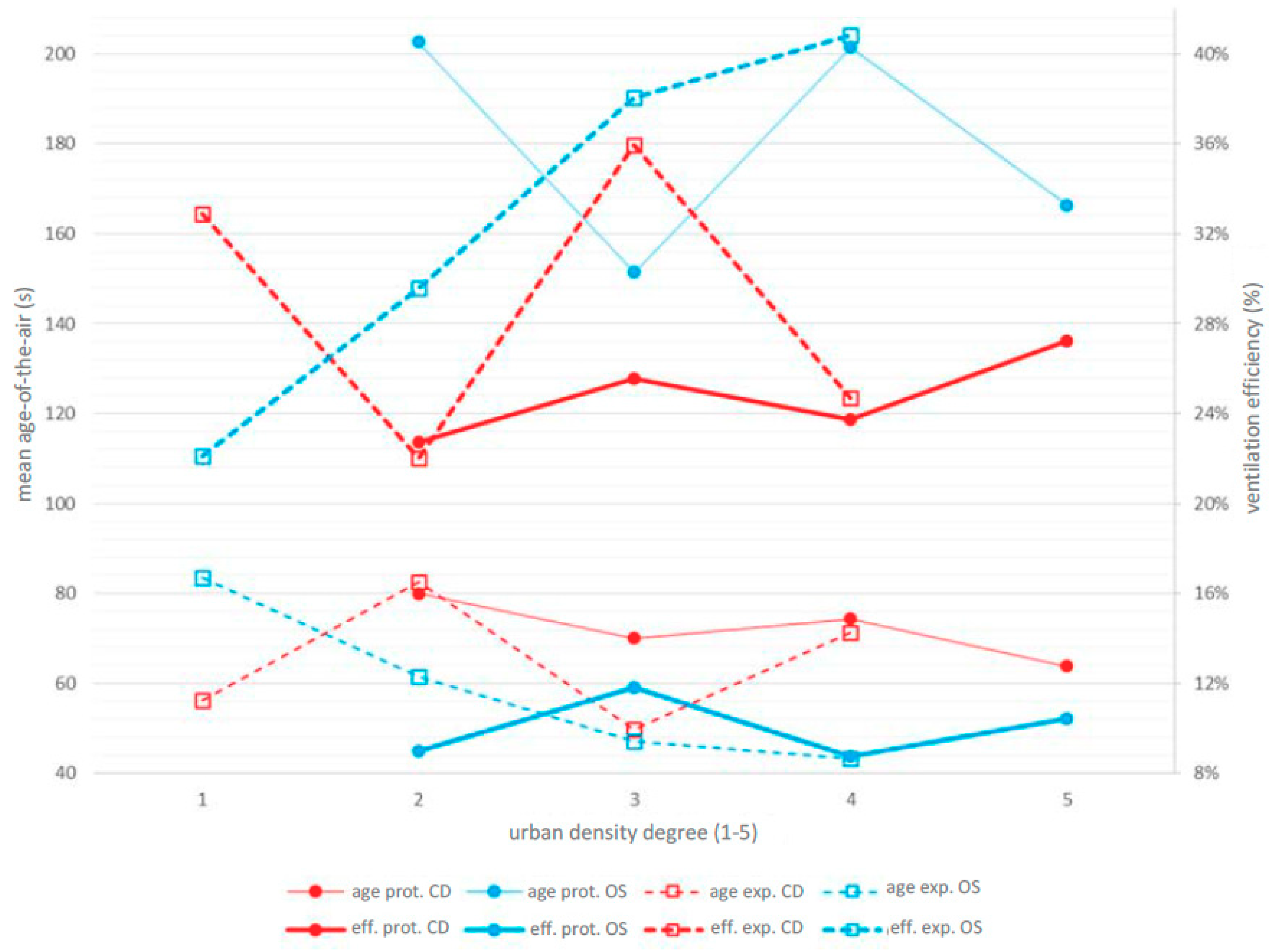
However, a pattern for confined outdoor spaces that are directly exposed to wind action can be established. The results (Figure 12) show that at higher urban densities the air change efficiency increases, considerably improving its capacity to renew the stale or contaminated air by improving the effect of homogeneous distribution of the air renewal. On the other hand, the higher the density, the lower the average age-of-the-air, which suggests an increase in the air flow as the volume of available air decreases.

In general, the obtained results show that the confined outdoor spaces which are exposed to the wind action are more predisposed to reduce the mean age-of-the-air of the air that they contain. It is observed that the most unfavourable case (reference case) is the one corresponding to Type e: protected intersection (G2p). The obtained results are related to the maximum ages of air and the minimum achieved efficiencies in the control domain and in the confined outdoor space, respectively (most unfavourable cases) (

Table 5. Age-of-the-air and air change efficiency improvement results regarding the most unfavourable situations.

Type of Confined Outdoor Space	Mean Age-Of-The-Air of the Control Domain	Mean Age-Of-The-Air of the Confined Outdoor Space	Air Change Efficiency of the Control Domain	Air Change Efficiency of the Confined Outdoor Space
G1e	31.96% (+29.75%)	58.79%	+10.84% (+10.11%)	+13.37% (+13.15%)
G2p *	3.15%	202.6 s	+0.73%	+0.22%
G2e	82.6 s (−3.25%)	69.64%	22.02% (−0.73%)	+20.80% (+20.58%)
G3p	15.13% (+12.38%)	25.27%	+3.53% (+2.80%)	+3.07% (+2.85%)
G3e	39.71% (+37.75%)	76.75%	+13.94% (+13.21%)	+29.29% (+29.07%)
G4p	10.05% (+7.13%)	0.56%	+1.73% (+1.00%)	8.76% (−0.22%)
G4e	13.56% (+10.75%)	78.68%	+2.68% (+1.95%)	+32.06% (+31.84%)
G5p	22.76% (+20.25%)	17.87%	+5.21% (+4.48%)	+1.68% (+1.46%)

Note: results in red are the most unfavourable; results in green are the most favourable regarding the reference values. * Values shaded in grey correspond to the reference case (G2p).

). The percentage differences regarding the reference case (G2p) are related in parentheses, this being the one that generally presents the worst results.

The urban design strategy has an important impact on the processes of outdoor air change and, therefore, of the air supplied to the buildings, being able to improve with the analysed guidelines. Easily applicable improvement is seen with urban models based on Type d: open exposed inner courtyard (G4e) or even on Type h: exposed urban corridor (parallel to the predominant wind orientation). These cases present improvements of 76.75% and 78.68%, respectively, in the age-of-the-air in the confined outdoor space and 32.06% and 29.29%, respectively, in the air change efficiency in the outdoor space, with regard to the most unfavourable case.

6. Conclusions

The phenomenon of outdoor air change in relation to the urban and architectural shape can considerably reduce the air conditioning energy consumption of the studied building. This implies the requirement of lower ventilation flow rates that mean the increase of the energetic demand to hygrothermally adapt the air coming from the urban environment to the characteristics of the building indoor air.

As it has been demonstrated, opting for solutions open to the predominant wind orientations in the site implies the improvement of the quality of the air to be introduced into the interior spaces of the buildings. However, it is not possible to define a unique pattern dependent on urban density for all generic cases. The analysis of the outdoor air quality according to the time that passes from its access to the urban environment in an ideal situation of purity and the time it takes for it to be supplied to the buildings allows us to evaluate in an approximate way the urban impact on the process of indoor ventilation. The longer the time is, the older the age-of-the-air is and, therefore, the more the air has been exposed to urban pollutants regardless of their source and intensity. A generic and simplified method to relate in a standardised way the urban design with its impact on air quality is proposed, evaluating also the capacity of the surrounding air to cause the necessary exchange with clean air.

Consequently, for the analysed cases, a considerable improvement of up to 78.68% in the quality of the air that is received in the buildings from the confined exterior spaces can be obtained, according to criteria of wind exposure in relation to space shape and urban density.