Abstract
Land based site selection for a wind farm has some challenging criteria, namely, cost for electricity generation and distribution, acquiring ownership of the site, potential barriers from various laws and permits, security concerns, access issues, feasibility of accommodation, etc. However, wind resource assessment deems the first criterion to rule out a site before other criteria can play roles in the selection process. In this paper, a Computational Fluid Dynamics (CFD) study has been performed on a complex mountainous terrain near a shore in the west coast of the US to assess the wind resource in order to spot potential suitable sites for wind turbines. Average wind speed at a height of 10 m at the centre (44°2212.0 N, 123°5924.0 W) of the chosen region under study has been compared with the simulated data for validation. Results from the study, which yields a continuous map of flow field variables, have revealed much more detailed features than the available state-wise wind maps. For example, it has revealed as high as 147% variation in wind speeds and 438% in wind power, making it possible to choose suitable sites without the need for, or perhaps in advance of, expensive direct measurements. This type of analysis may help in preliminary assessments and expedite the site selection process.
1. Introduction
Energy demand is increasing around the world due to industrialization and development, and fossil fuels have been the major player to provide this energy. However, its negative impact on environment and thus climate change has been a topic of discussion for decades. Burning fossil fuel produces CO, CO, and other toxic gases that affect health and environment such as causing respiratory diseases and global warming, respectively.
Renewable Energy Sources (RES) are not only an alternative to conventional fossil fuel but can also provide power for the electricity deprived regions (where electricity supply from national grid is limited for installation costs and maintenance) as in many rural and hilly areas in many countries and areas hit by natural disasters.
The clean energy market has been expanding gradually and has managed to reduce profits of fossil fuel companies. It has grown nearly six times compared to its business in 2004 by totalling about $329 billion in investment [1]. Awareness of governments around the world and support from corporations and the public alike have made it possible to cut down clean energy cost over years. Government incentives have played a major role in this scenario. For example, large-scale solar energy and wind energy cost have reduced by 60 percent and 40 percent, respectively, since 2008 [2]. People living in rural and mountainous areas not connected with the central grid have pursued solar energy as a quicker and less expensive option. Corporations have come forward by cutting down heat-trapping gas emissions and putting a price on carbon [1].
Wind is one of the RES that is always available free and wind power plants do not emit any air or water but noise pollution. Cumulative wind capacity around the world has been reported in 2018 to have seen a growth from 23,900 megawatts in 2001 to 539,581 megawatts in 2017 with an average annual increase of 25 percent over the past decade [3].
The crucial factor in developing any large- or small-scale wind farms is to assess wind resources accurately and characterize them properly. An assessment of wind resource in 2009 [4] has reported that the land-based wind energy has a potential of generating power of 10,500 GW (gigawatt) at 80 m and 12,000 GW at 100 m with a capacity factor of at least 30 percent in the USA.
The National Renewable Energy Laboratory (NREL) has been a dedicated US government organization to develop and manage wind farms through its research and data collection, where US based characterized wind map are available. Figure 1 from NREL is a presentation of a characterized wind map based on the annual average wind speed at 80 m height above sea-level. This map has been constructed with a low resolution (2.5 km ≈ 1.24274 mile) data recording and then the data have been interpolated to a finer resolution [5]. This type of categorized wind map helps find target regions for consideration within seconds to build large-scale wind farms.
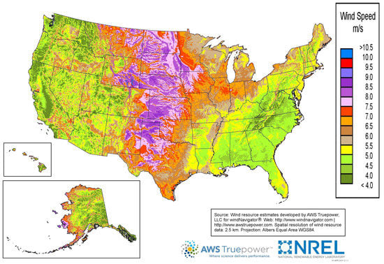
Figure 1.
Annual average wind speed of the US at 80 m [5].
State-wise wind maps are also featured in NREL website. Figure 2 presents a similar wind map of California, USA based on the annual average speed at 30 m. It has been developed similarly with recorded data of spatial resolution of 2.0 km and then filled up with finer resolution via interpolation algorithm. This map definitely gives a good colored characterized wind speed distribution over the state. However, it still lacks the necessary resolution needed to accurately spot potential regions with suitable wind speed if a small region (a city, a county, or a village) is picked for consideration of small scale installation.
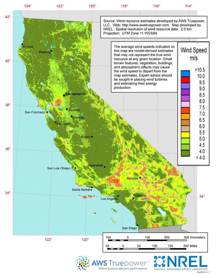
Figure 2.
Annual average wind speed of California at 30 m [6].
To find wind resource sites, GIS (Geographic Information System) based MCDM (Multi Criteria Decision Method) is a very useful tool if numerous data points (e.g., terrain, wind resource, etc.) are available [7,8]. Categorized wind map may not be available for all locations especially for remote and complex mountainous terrains. Computational Fluid Dynamics (CFD) software packages have been employed to analyze micro-scale and meso-scale sites [9,10] to characterize winds and model wind farms [11,12]. However, repetitive wind analysis may become a common practice in the near future as the world is leaning towards renewable energy and urbanization keeps changing the demography and city structures every few years. To adapt the situation, small and large scale power plants (solar, wind and other renewable energy sources) are likely to be constructed in a large number. A detailed high resolution wind map is undeniably an essential tool in this scenario.
This paper uses OpenFOAM (Open source Field Operation And Manipulation), an open-source CFD software package, to generate various fluid flow property maps (e.g., velocity, pressure, turbulence kinetic energy, etc.) over a meso-scale 17.5 km × 11.12 km complex mountainous terrain in Oregon as a case study in search of potential small-scale wind turbine (especially Vertical Axis Wind Turbine) candidate sites where high resolution wind data are not currently available. Use of meso-scale simulations such as this may not provide the granularity of micro-scale simulations but do improve upon, with respect to resolution, the currently available wind maps from NREL, for example. It may be possible to use such a tool to improve resolution on national-scale wind maps.
2. CFD Modeling
2.1. Computational Domain
The domain has been modeled as a rectangular prism, the six sides of which correspond to the phenomena in the real site, i.e., the top as sky, the bottom as ground, the inlet as the face the wind is entering through, the outlet as the face the wind is leaving through, and the sides as the faces which experience no variation in their normal direction (properties remain same on both sides) (Figure 3). The origin “O” and the Cartesian coordinate system shows the orientation of the domain.
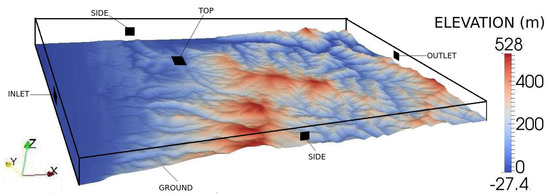
Figure 3.
Computational domain and the colored ground is showing elevation above sea-level.
The scale of simulation investigated herein can be assumed of having no Coriolis force effects [13]. The equations of motion are governed by steady state Reynolds-Average Navier–Stokes (RANS) equations in the domain. The fluid is wind at the standard atmospheric temperature which can be assumed to be incompressible. Other thermo-physical effects (e.g., gravity) are negligible. The chosen site is designated by latitude and longitude and elevation h, which is the height above sea-level. This information needs to be transformed into points (or vertices) in three dimensional space () for blockMesh to use in formation of cell blocks. The coordinate of each point in the computational domain is bounded by and . Following the origin in Figure 3, mapping of vertices can be described as follows:
where m is the radius of the earth. The domain is almost rectangular and the top boundary is chosen at a height, H, far enough away from the ground not to affect the solution.
Blocks are formed from the coordinates of points (or vertices) with height from to while the subdivided cell volumes along the height vary with an expansion ratio, , as follows:
where is the end cell thickness and is the starting cell thickness in the z-direction. Intermediate cells have linearly interpolated thickness.
2.2. Governing Equations
The equation of conservation of mass is written as
and the equation of conservation of momentum can be written as
where is the time-averaged fluid velocity and two tensors- and are the mean strain rate tensor and the specific Reynolds stress tensor, respectively. is derived from the fluctuation of velocity. These tensors can be expressed as:
2.3. Turbulence Model
A turbulence model needs to be adopted to address this specific Reynolds stress tensor, . Several models have been developed which base on Boussinesq hypothesis that assumes varies linearly with the mean velocity gradients and thus introduces two other quantities in the expression of : (a) turbulence kinetic energy, ; and (b) kinetic eddy viscosity, .
In this paper, the model has been used as used in other larger scale simulations such as wind turbine simulations [14,15]. The standard model is a two-equation model as it requires solution of two transport equations to achieve closure and deliver accurate enough predictions. It brings in another term, , the rate of dissipation of per unit mass due to viscous stresses to establish relationship between and .
where = 0.09 is a constant. The stead-state transport equations for and can be written as:
where = 1.44, = 1.92, = 1.0, and = 1.3 are typical recommended values for this turbulence model.
2.4. Solution Algorithm
An algorithm is needed to solve the system of equations with proper boundary and initial conditions. SIMPLE (Semi-Implicit Method for Pressure Linked Equations), a widely used Navier–Stokes Equations’ solver, has been chosen for the current steady state fluid flow case in question. OpenFOAM has named the solver “simpleFoam”.
2.5. Boundary Conditions
The boundary conditions mimic the phenomena of the chosen site such as the air flows in the x-direction as it enters the region of interest but its speed varies with height. Therefore, a power-law relationship describing the speed of air with height is employed to model the wind speed profile. This power-law relationship is frequently used to measure power densities of wind and macroscopic wind velocity [16,17]. The relationship can be shown as:
where a is a constant equal to or 0.143, is a reference wind speed measured at a height, h, and z is the elevation in meters. The chosen value as 1/7 is aimed at coinciding with flat near-ocean region [18] as the inlet. Obviously, choosing other values of “a”, such as 0.1, will definitely change the inlet wind profile. However, the results, which rely more on flow field comparisons than on absolute value, should remain valid regardless of (reasonable) choice of “a”. All other boundaries but the inlet are set to a zero velocity-gradient boundary condition that acts on the normal direction of boundary surfaces:
where is the outward pointing surface normal. Pressure is forced to have a value of zero at the outlet.
On all other boundaries, a zero gradient boundary condition normal to the surface is invoked.
An important point is to be noted at this stage is that the unit of the pressure is due to its division by density, , that facilitates the solution of the governing equations in the incompressible solvers. To initialize, pressure is chosen arbitrarily to be used everywhere since only the relative pressure difference is taken into account. Turbulence kinetic energy, k, can be expressed as follows:
where I is the turbulence intensity. The other boundaries have similar zero-gradient boundary condition normal to their surfaces.
Rate of turbulence dissipation can be written as:
where l is the turbulence length scale that approximates to the average of the length of cell volumes in ground discretization. Other boundaries are again enforced to have zero-gradient boundary condition normal to their surfaces.
2.6. Simulation Software
The governing equations along with sufficiently described boundary and initial conditions are solved using OpenFOAM [19], a finite volume based C++ toolbox capable of solving a wide range of multi-physics problems including CFD. The domain is descritized by blockMesh, a native meshing tool that comes with the OpenFOAM package. The vertices of grid elements are used to form blocks and then cell volumes are created from the subdivision of those blocks.
3. Case Study and Validation
The chosen site is of length 17.507 km (8.75 miles) and width 11.12 km (6.67 miles) approximately and is shown in Figure 4 and the elevation data have been collected from Google [20].
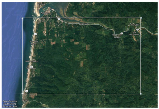
Figure 4.
The boxed area under investigation, adapted from Google Earth [21]. It lies within ∈ (44.32, 44.42) and ∈ (−124.11, −123.89).
The ground of domain in Figure 3 shows the topography of the chosen mountainous terrain. The redder locations have greater elevation while the bluer areas are closer to sea-level.
The air properties have been taken as the standard values at room temperature and at sea-level such as air density, = 1.2 kg/m, and dynamic viscosity, = 1.8 kg/ms. The turbulence intensity, I, is taken as 1% or 0.01.The real time velocities at six points (plus four points around the validation point) on the area under investigation have been collected from OpenWeatherMap [22] for 24 h starting on 24 June 24 2017 at 2:35 a.m. (UTC). The reference velocity, , is calculated as 4.1 m/s. This value comes as an average of the recorded velocities at six observation points, as shown in Figure 5. The distribution of velocities in Figure 5b is of Point 1 only. The other points show similar trends. The inlet reference velocity is taken as the average of speeds at all six points over the period of 24 h. Despite the availability of standard registered data (i.e., wind maps), preference was given to record the wind speeds to observe if there was any considerable difference and the calculated velocity is (Figure 6) reasonably close to the standard.
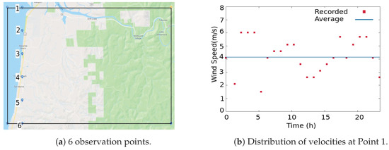
Figure 5.
Inlet velocity.
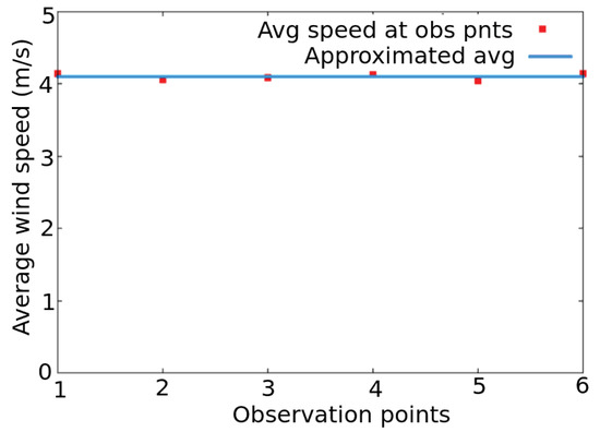
Figure 6.
Average inlet reference velocity.
The computational domain is made up of 200 × 125 nodes. The average side length of cell volumes gives an estimated turbulence length scale of 44.12 m. The ceiling of the domain in Figure 3 is at 1000 m away from sea-level.
A grid independence test (Figure 7) has been conducted to ensure that results do not vary with grid size in the domain. Several simulations have been run using various mesh sizes and velocity in the x-direction has been compared with the recorded data as a measurement of success. The simulation result with 1.92 million cells seems to match with the collected data perfectly, but does not remain consistent with increased number of cells (for example, 3.2 million). Therefore, it can be inferred that this particular result is very prone to errors because of comparatively low resolution of the computational domain and thus should be avoided. The mesh size that is chosen eventually to conduct the study is of cells.
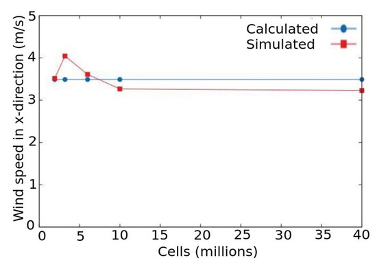
Figure 7.
Grid independence test and validation.
The wind is never unidirectional and uniform. However, the recorded velocities have orientations around 350∼ 360. Therefore, the wind velocities have been just time-averaged to determine the inlet velocity and it has been considered to be unidirectional for simplification. In addition, the record does not include wind speed in z-direction as it is assumed to be very low and cannot impact this study to a considerable level.
The OpenWeatherMap [22] collects data from airport, public and private weather stations and they are not necessarily calibrated for the same height which may explain some of the variations in Figure 5b. However, most of these are calibrated to a height to 10 m. Data for each station have not been tracked and recorded separately. Therefore, chances of stations’ data for a height other than 10 m remain, although these stations can be considered small in number. However, averaging data reduces this error to a negligible level.
Each block in the domain has 100 cells in z-direction with a cell expansion ratio = 750 and two cell volumes in x and y directions.
The simulation was then run using a linear 2nd order, cell-centered finite volume spatial discretization with a relative residual tolerance less than for u, v, w, p, and solvers.
4. Results and Discussion
The objective of this study is to generate a wind map of a region to spot locations as potential wind resource sites. It also varies to some extent, if not significantly, at different elevations depending on the topographical features of the area. Therefore, wind maps of Oregon, USA (where the area under investigation is located) at 30 m and 80 m have been the bases for comparison with the flow properties of air from the simulation.
4.1. Wind Flow Properties at 30 m
Figure 8 presents a characterized wind map of Oregon, USA from NREL [23]. The red dot on the map (shown with the arrow for better visualization) is the region of interest for the current study. It can be easily concluded from the map that most of the state has an annual average wind speed of 4–5 m/s. In addition, the resolution has been interpolated from a 2.0 km grid to finer grids. Therefore, trying to characterize wind on any particular small area using this wind map is challenging and results will be prone to errors.
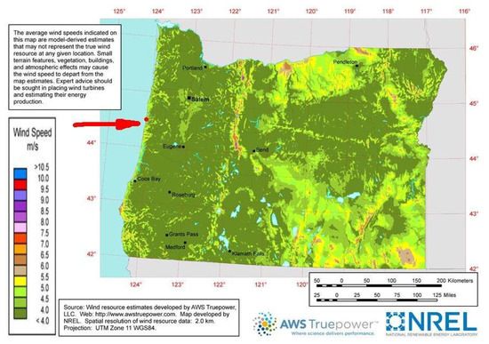
Figure 8.
Average annual wind speed of Oregon at 30 m.
The flow velocity in x-direction (,) from left to right is positive. Figure 9 shows distribution of the region at 30 m above ground. The inflow comes from the left and being a flatter region; this portion of the region has mostly a similar velocity as the inlet. However, there are considerable number of locations where it drops too low (even negative) and, at some other locations, rises to high. Any blockage in the flow path in the form of hills or cliffs can make the flow stop and turn, which reduces the speed. On the other hand, air flows faster through a narrow passage (such as valley) or over water body as the friction of water is less than that in solid surfaces.
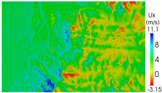
Figure 9.
Wind speed in x-direction at 30 m.
The flow velocity components are combined together to get its magnitude that has been produced in Figure 10a. NREL suggests that at 30 m height a velocity magnitude of 4 m/s or higher is suitable for wind farm [24]. The pie chart of area distribution (Figure 10b) shows that almost 67% area of the region meets the minimum target. Other categorized wind speed zone can by pointed out and its area share can be known from Figure 10.
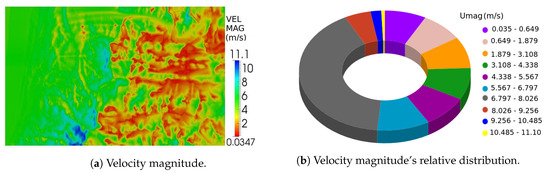
Figure 10.
Velocity magnitude at 30 m.
The inflow is completely unidirectional ( = 0, = 0 at inlet). Thus, and components come from wind shear, turbulence, wake propagation, change in flow path due to blockages, etc. Figure 11a reveals spots with positive and negative where bluish and reddish regions are two extremes respectively. This gives the idea about where the turning of flow direction is likely to occur and thus topographical feature of those spots can be guessed. Likewise, Figure 11b reveals spots where vertical turnings of flow occur as it passes over and through the terrain. Slopes will likely produce positive while cliffs or cliff-like blocks will generate negative .
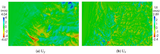
Figure 11.
Velocity components in y- and z-direction at 30 m.
Turbulence causes fatigue loading on turbine blades, i.e., time varying torque and thrust that reduces turbine’s longevity. Turbulent flow has random wind velocities and is quantified by turbulent kinetic energy (TKE), . Figure 12 shows distribution of at 30 m. As shown in the figure, the vicinity near the inlet has higher because of the viscous effect from solid surface friction and thick turbulent boundary layer. As the flow nears the mountainous terrain, the eddies decay as they approach solid surfaces of the terrain.
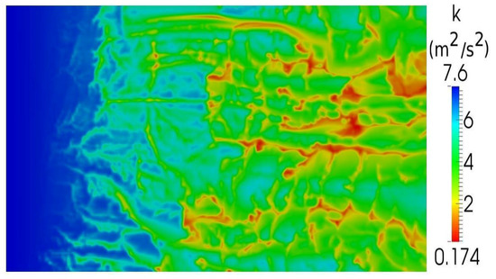
Figure 12.
Turbulence kinetic energy distribution at 30 m.
Wind power density is proportional to and thus depends on the magnitude of velocity and is considered as an important criterion for assessment of a region for potential wind resource. Here, wind power density has been calculated as per m area. Figure 13a has been produced to observe wind power distribution over the region. The pie chart in Figure 13b shows percentage of area share of wind power densities. The maximum value that can be found as 294.1 W/m which is 5.4 times higher than the minimum required average wind power density (54.675 W/m).
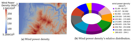
Figure 13.
Wind power density at 30 m.
4.2. Wind Flow Properties at 80 m
Oregon’s wind map from NREL [25] is shown again in Figure 14 at 80 m and, at this elevation, 6.5 m/s or higher wind speed is suitable for wind farms [26]. The blue dot shows the location that our study has focused on. Again, this map gives an overall idea about the average wind speed throughout the state but lacks the details to use it for meso- or micro-level location analysis for potential wind resource.
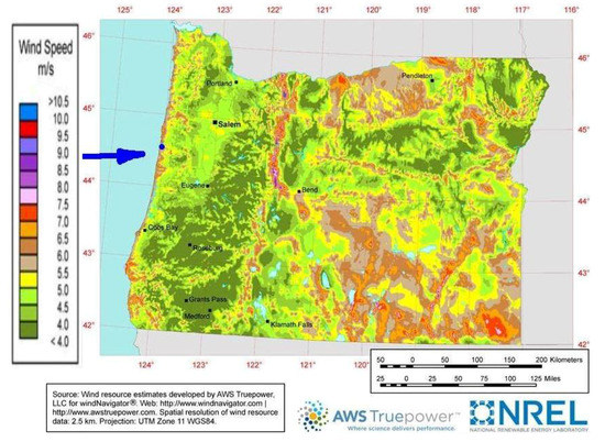
Figure 14.
Average annual wind speed of Oregon at 80 m.
Since the inflow is in direction, this velocity component, i.e., , is larger than the other two and its distribution is shown in Figure 15. At this elevation, areas with higher velocities (blue regions) are larger than those at 30 m and areas with lower velocities (red regions) are lesser than those at 30 m. It is obvious that blockage in the flow path decrease with the increase of height.
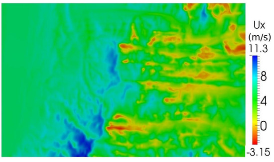
Figure 15.
Wind speed in x-direction at 80 m.
Similarly, (Figure 16a) and (Figure 16b) maps show how these velocity components change with elevation. Both bluish (+) and reddish (-) regions reduce in size in comparison with the map for 30 m. It is true for as well. The reason definitely can be attributed to less deflection and thus less blockage in the flow path.
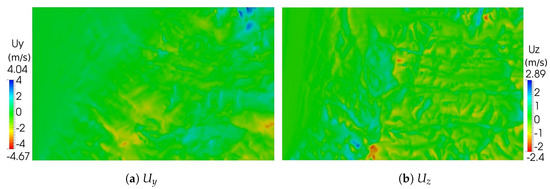
Figure 16.
Velocity components in y- and z-direction at 80 m.
Velocity magnitude and its pie chart have been produced in Figure 17. A barchart (Figure 18) summarizes the comparison of wind speeds at two different elevations. The percentage of areas with higher speeds are larger at 80 m. The maximum velocity found at 80 m is also higher than that at 30 m.
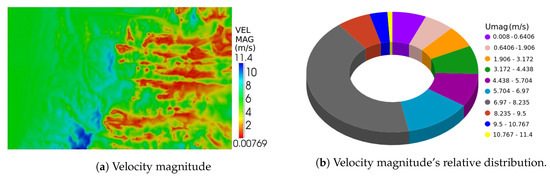
Figure 17.
Velocity magnitude at 80 m.
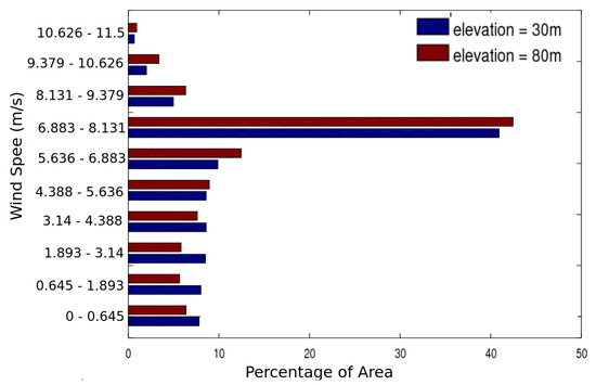
Figure 18.
Wind speed’s relative distribution by areas at two elevations.
Turbulent kinetic energy (TKE) map in Figure 19 for the height of 80 m shows that regions with higher turbulence have increased in size in comparison with the map at 30 m. The region near the inlet experiences more turbulence as wind shear affects flow at different layers within thick turbulent boundary layer. The mountainous terrain has also higher since there are less solid surfaces for the eddies to decay, rather wind shear contributes to the eddies.
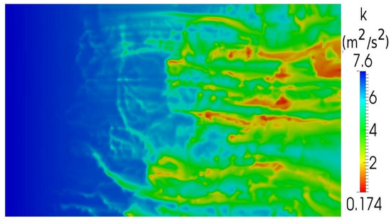
Figure 19.
Turbulence kinetic energy distribution at 80 m.
Figure 20 shows the wind power distribution on the region at 80 m. The pie chart (Figure 20b) shows percentage of area share of different wind power densities. To compare it with wind power density at 30 m, Figure 21 has been added. The magnitude of maximum wind power density is higher at 80 m. Regions with higher wind power have more percentage in comparison to those at 30 m. NREL recommends a site should have as low as 185 W/m wind power density to qualify while we get a wind power density as high as 305 W/m, which is 1.65 times higher.
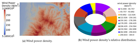
Figure 20.
Wind power density at 80 m.
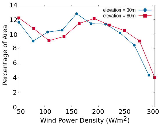
Figure 21.
Wind power density’s relative distribution by areas at two elevations.
5. Conclusions
Site selection for wind farms involves a few important criteria such as cost for power generation and distribution, ownership of the site, limitations due to laws and permits, security, accessibility, feasibility, and so on but the major one is the availability of wind source. This study shows a CFD approach to identify possible site selection.
The current study has adopted an approach to model a meso-scale simulation with an open-source CFD software, OpenFOAM, and has utilized the standard turbulence model. By using terrain elevation data from Google and the wind profile (power law), steady-state solution has been simulated and then flow field variables have been analyzed. To better understand the effect of altitude on the variables better, results have been analyzed at two different altitudes (30 m and 80 m).
The results demonstrate that the state-wise wind map may be useful for large wind energy projects, but may not be as useful for small scale installations. The area investigated herein is rectangular and spans 17.507 km in length and 11.12 km in width. Due to the resolution of typical wind maps, it is difficult to gauge how small-scale topographical variations can contribute to wind energy availability.
By observing the wind maps of Oregon from NREL, the region under the current study is assumed to have an annual average wind speed of about 4.5∼5.0 m/s at 30 m and 6.0∼6.5 m/s at 80 m , however, our study reveals much more variation in wind speed and wind energy density. Our results indicate several locations within this region that are unsuitable for wind energy conversion due to relatively low wind speeds. Conversely, several other locations are highly recommended as candidate sites where average wind speeds are up to 147% higher than the NREL average at 30 m and 75% higher at 80 m. The results suggest that using meso-scale CFD simulations on areas of interest could greatly help in forming wind maps of smaller regions and potentially larger regions.
Although this study uses recorded wind speed data on the span of 24 h to provide inlet boundary conditions, this type of analysis could be used with long-term recorded data to provide more accurate results, and perhaps identify sites not realized through analysis of currently available, large-scale wind resource maps.
Author Contributions
D.M. conceptualized and acquired Funding; L.R. collected data, carried out the simulation, validated, analyzed, wrote and edited the article primarily; D.M. supervised the project, reviewed, and helped edit the article.
Acknowledgments
This work was supported by the Applied Computational Engineering (ACE) Lab at the University of Alabama.
Conflicts of Interest
The authors declare no conflict of interest.
References
- MacDonald, J. Clean Energy Defies Fossil Fuel Price Crash to Attract Record $329BN Global Investment in 2015. Available online: https://data.bloomberglp.com/bnef/sites/4/2016/01/BNEF-2015-Annual-Investment-Numbers-FINAL.pdf (accessed on 6 April 2018).
- Revolution Now: The Future Arrives for Five Clean Energy Technologies—2015 Update. Available online: https://www.energy.gov/sites/prod/files/2015/11/f27/Revolution-Now-11132015.pdf (accessed on 6 April 2018).
- Global Wind Statistics. 2017. Available online: http://gwec.net/wp-content/uploads/vip/GWEC_PRstats2017_EN-003_FINAL.pdf (accessed on 6 April 2018).
- Wind Resource Assessment and Characterization. Available online: https://energy.gov/eere/wind/wind-resource-assessment-and-characterization (accessed on 6 April 2018).
- Wind Maps. Available online: https://www.nrel.gov/gis/images/80m_wind/USwind300dpe4-11.jpg (accessed on 6 April 2018).
- Wind Energy Maps and Data. Available online: https://windexchange.energy.gov/files/u/visualization/image/ca_30m.jpg (accessed on 6 April 2018).
- Latinopoulos, D.; Kechagia, K. A GIS-Based Multi-Criteria Evaluation for Wind Farm Site Selection: A Regional Scale Application in Greece. Renew. Energy 2015, 78, 550–560. [Google Scholar] [CrossRef]
- Haaren, R.V.; Fthenakis, V. GIS-based Wind Farm Site Selection Using Spatial Multi-criteria Analysis (smca): Evaluating the Case for New York State. Renew. Sustain. Energy Rev. 2011, 15, 3332–3340. [Google Scholar] [CrossRef]
- Liu, X.; Yan, S.; Mu, Y.; Chen, X.; Shi, S. CFD and Experimental Studies on Wind Turbines in Complex Terrain by Improved Actuator Disk Method. J. Phys. Conf. Ser. 2017, 854, 012028. [Google Scholar] [CrossRef]
- Li, B.; Zuo, L.; Li, J.; Wang, P.; Liang, H.; Huang, Q. Simulation-Based Micro-Site Selection for Wind Farm in Complex Terrain. In Proceedings of the IEEE International Conference on Smart Grid and Clean Energy Technologies (UESTC), Chengdu, China, 19–22 October 2016; pp. 196–200. [Google Scholar]
- Ayala, M.; Maldonado, M.; Paccha, E.; Riba, C. Wind Power Resource Assessment in Complex Terrain: Villonaco Case-Study Using Computational Fluid Dynamics Analysis. Energy Procedia 2017, 107, 41–48. [Google Scholar] [CrossRef]
- Avila, M.; Folch, A.; Houzeaux, G.; Eguzkitza, B.; Prieto, L.; Cabezón, D. A Parallel CFD Model for Wind Farms. Procedia Comput. Sci. 2013, 18, 2157–2166. [Google Scholar] [CrossRef]
- Forthofer, J.M. Modeling Wind in Complex Terrain for Use in Fire Spread Prediction. Ph.D. Thesis, Colorado State University, Fort Collins, CO, USA, 11 May 2007. [Google Scholar]
- Franco, J.A.; Jauregui, J.C.; Toledano, A.M. Optimizing Wind Turbine Efficiency by Deformable Structures in Smart Blades. JERT 2015, 137, 051206. [Google Scholar] [CrossRef]
- Jackson, R.S.; Amano, R. Experimental Study and Simulation of A Small-Scale Horizontal-Axis Wind Turbine. JERT 2017, 139, 051207. [Google Scholar] [CrossRef]
- Blocken, B.; Carmeliet, J.; Stathopoulos, T. CFD Evaluation of Wind Speed Conditions in Passages Between Parallel Buildings—Effect of Wall-Function Roughness Modifications for the Atmospheric Boundary Layer Flow. JWEIA 2007, 95, 941–962. [Google Scholar] [CrossRef]
- Meroney, R.N.; Leitl, B.M.; Rafailidis, S.; Schatzmann, M. Wind-Tunnel and Numerical Modeling of Flow and Dispersion About Several Building Shapes. JWEIA 1999, 81, 333–345. [Google Scholar] [CrossRef]
- Bechrakis, D.A.; Sparis, P.D. Simulation of The Wind Speed at Different Heights Using Artificial Neural Networks. Wind Eng. 2000, 24, 127–136. [Google Scholar] [CrossRef]
- Jasak, H.; Jemcov, A. OpenFOAM: A C++ library for complex physics simulations. In Proceedings of the International Workshop on Coupled Methods in Numerical Dynamics IUC, Dubrovnik, Croatia, 19–21 September 2007; pp. 1–20. [Google Scholar]
- Elevation API. Available online: https://developers.google.com/maps/documentation/elevation/start (accessed on 6 April 2018).
- Google Maps. Available online: https://www.google.com/maps/place/44%C2%B019’12.0%22N+124%C2%B006’36.0%22W/@43.2217455,-122.5167258,1499555m/data=\protect\kern-.1667em\relax3m1\protect\kern-.1667em\relax1e3\protect\kern-.1667em\relax4m5\protect\kern-.1667em\relax3m4\protect\kern-.1667em\relax1s0x0:0x0\protect\kern-.1667em\relax8m2\protect\kern-.1667em\relax3d44.32\protect\kern-.1667em\relax4d-124.11 (accessed on 6 April 2018).
- Current Weather Data. Available online: https://openweathermap.org/current#one (accessed on 6 April 2018).
- Wind Energy Maps and Data. Available online: https://windexchange.energy.gov/files/u/visualization/image/or_30m.jpg (accessed on 6 April 2018).
- Wind Energy Maps and Data. Available online: https://windexchange.energy.gov/maps-data/216 (accessed on 6 April 2018).
- Wind Energy Maps and Data. Available online: https://windexchange.energy.gov/files/u/visualization/image/or_80m.jpg (accessed on 6 April 2018).
- Wind Energy Maps and Data. Available online: https://windexchange.energy.gov/maps-data/104 (accessed on 6 April 2018).
© 2018 by the authors. Licensee MDPI, Basel, Switzerland. This article is an open access article distributed under the terms and conditions of the Creative Commons Attribution (CC BY) license (http://creativecommons.org/licenses/by/4.0/).