Biogas and Ethanol from Wheat Grain or Straw: Is There a Trade-Off between Climate Impact, Avoidance of iLUC and Production Cost?

Abstract

Current EU policy calls for decreased emissions of greenhouse gases (GHG) by i.e., replacing fossil fuel in the transportation sector with sustainable biofuels. To avoid indirect land use change (iLUC), the EU at the same time strives to limit the use of crops and to increase the use of residues. In this study we compare climate impact and production cost for biogas and ethanol based on wheat grain and straw, respectively, in a Swedish context. The economic competitiveness for ethanol from straw vs. grain is evaluated based on the mandatory emission reduction for fossil vehicle fuels implemented since July 2018 in Sweden. The result of this study clearly shows that biogas and ethanol from straw have the lowest GHG emissions regardless of the calculation method used, although biofuels from grain also fulfill EU GHG reduction criteria even when suggested iLUC factors are included. It was also shown that the cost of producing straw-based biofuels was higher, thus there is a trade-off between climate impact and costs. The GHG reduction mandate adopted in Sweden partly compensates for this, but is not enough to make ethanol from straw competitive from an economic perspective.

1. Introduction

According to EU policy, greenhouse gas (GHG) emissions need to be reduced by 40% by 2030 compared to the levels in 1990 [1]. By 2015, the member states had achieved an average emission reduction of 24%. However, emissions from the transportation sector, representing 20% of total GHG emissions, have increased by 16% during the same period [2]. It is thus important to address these emissions if we are to achieve the overall EU GHG emissions target.

The Swedish parliament has approved a new climate policy which includes, among other things, the goal of net zero GHG emissions in Sweden by 2045 [3]. The goal set for emissions from the domestic transport sector (excluding aviation) is a reduction of at least 70% by 2030, compared with 2010. In order to achieve these targets, a combination of several measures such as reducing the need for transportation, improving energy efficiency and electrification, as well as the increased use of biofuels are required [4].

The EU has also set a mandatory target of 10% sustainable biofuels in the transportation sector in each Member State by 2020 [5]. Based on the method of calculation given in the EU renewable energy directive (RED), the average fraction of biofuels used in 2015 was 6.7% [6]. Sweden has the highest proportion of renewable transportation fuels in the EU (24%). However, more than 90% of the biofuel consumed in Sweden is imported [7]. With an increasing demand for biofuels in other countries, it seems unlikely that Sweden would be able to continue to import the increasing amount needed in the future. Thus, an increase in the consumption of biofuels calls for a considerably higher level of domestic production than today.

Current EU policy requires that the production of biofuels be sustainable, which means, for example, that GHG emissions arising from the production of biofuels in new plants must not exceed 40% of the emissions from fossil vehicle fuels or 33.5 g CO₂eq MJ⁻¹. In recent amendments, EU policy also focusses on reducing the use of crops as feedstock for biofuel production, and increasing the use of residues. Member States are only allowed to use 7% biofuels from crops to meet the mandatory target of 10% sustainable biofuels mentioned above. One reason for this is the concern that changes in land use might cause additional GHG emissions [8].

Changes in land use are often divided into direct land use change (dLUC) and indirect land use change (iLUC). The former term is used when land is converted from one state to another to grow biofuel crops (e.g., clearing forest to grow wheat for making ethanol). The latter describes the changes in land use that take place, for example, as a consequence of a bioenergy project, but which is not geographically connected to it. The reasoning behind this is theoretical; if biofuel crops are cultivated on existing agricultural land this might displace other crop production, causing a change in land use elsewhere. The effects of iLUC are closely associated with the demand and supply of agricultural commodities, and the change in market behaviour that can be triggered by biofuel projects [9].

Due to the much debated issue of land use, the EU has amended the RED, adding so called iLUC factors, to impose a GHG emission penalty on the use of certain feedstocks, such as cereals and other starch-rich crops, sugar and oil crops, for biofuel production. The iLUC factor for ethanol produced from cereals is 12 g CO₂eq MJ⁻¹ biofuel. However, the quantification of these iLUC factors has been criticized, as the economic equilibrium models used are complex optimization models based on the assumption of perfect markets involving numerous assumptions. Also, the results from different studies vary considerably [9]. According to Popp et al., it is also common that the positive impact of co-products that can be used as feed is underestimated [10]. Several alternatives to these economic models have been developed, often based on a causal descriptive or normative approach. These approaches tend to be simpler than economic models, and require less data, however, they are less detailed and therefore have higher uncertainties [11]. An overview of the causal descriptive models used to estimate iLUC can be found in Ahlgren et al. [12].

Straw is an agricultural residue, not a food crop, so the above arguments do not apply. However, the iLUC concept is closely associated with demand and supply of agricultural products. If straw has a current use, e.g., as bedding material, it could be replaced by other products e.g., sawdust, triggering market ripple effects, which could lead to additional GHG emissions. Using straw that would otherwise be left on the field to decay, and that is not required for soil organic carbon maintenance, will have no iLUC effect [13,14]. However, if straw is utilized in the future for biofuel production, a market demand will develop. There may also be a demand for straw as feedstock for the production of chemicals, bio-plastics, textiles, pharmaceuticals, etc. The question is, for how long time straw can be considered to be “iLUC-free”. In this study, we have assumed that straw has no iLUC effect, mainly due to the lack of methods of quantifying these effects.

Since one of the main objectives with biofuels is a reduction in overall GHG emissions, it is important to include direct as well as indirect effects in any analysis. Even if some feedstocks are considered “iLUC-free”, biofuels from these feedstocks do not necessarily have the lowest GHG emissions if direct and indirect effects are included.

Since the implementation of biofuels also calls for appropriate policy instruments, a detailed understanding of the various contributions to the cost of biofuel production is necessary. For example, Sweden is implementing a new policy instrument for low-blend renewable vehicle fuels by which suppliers of fossil vehicle fuels are obliged to cut GHG emissions by a certain percentage each year by blending in biofuels. For petrol, the reference value has been set to 93.3 g CO₂eq MJ⁻¹, and the required emission reduction in 2020 will be 4.2%. Since the GHG mandate is defined in terms of an emissions reduction and not the volume of biofuel, this policy instrument favours biofuels with low emissions. If the supplier does not meet this obligation, the penalty will be up to €0.8 kg⁻¹ CO₂-eq. [15].

In this study, the GHG emissions and production costs of four different biofuel production systems were analysed. The main kinds of domestic biofuel production in Sweden today are biogas based on waste and residues and ethanol based on cereal grain. Bearing in mind current EU restrictions on the production of biofuels from crops, and that Swedish regulation favours biofuels with low GHG emissions, we compared the use of wheat straw to the use of wheat grain as feedstock for ethanol and biogas production in a Swedish context. The purpose is to identify drawbacks and benefits if residues are prioritized over energy crops for the production of biofuels. To exemplify how reduced GHG emissions could be given an economic value, the results are also applied in the context of the Swedish GHG reduction mandate. Thus, the cost for the mandatory emission reduction is calculated using ethanol from grain versus straw applying the production cost and GHG emissions calculated in this study.

2. Materials and Methods

The study was based on a range of method applications and data inventories, which are summarized here, and further described in the following sections or in the appendices:

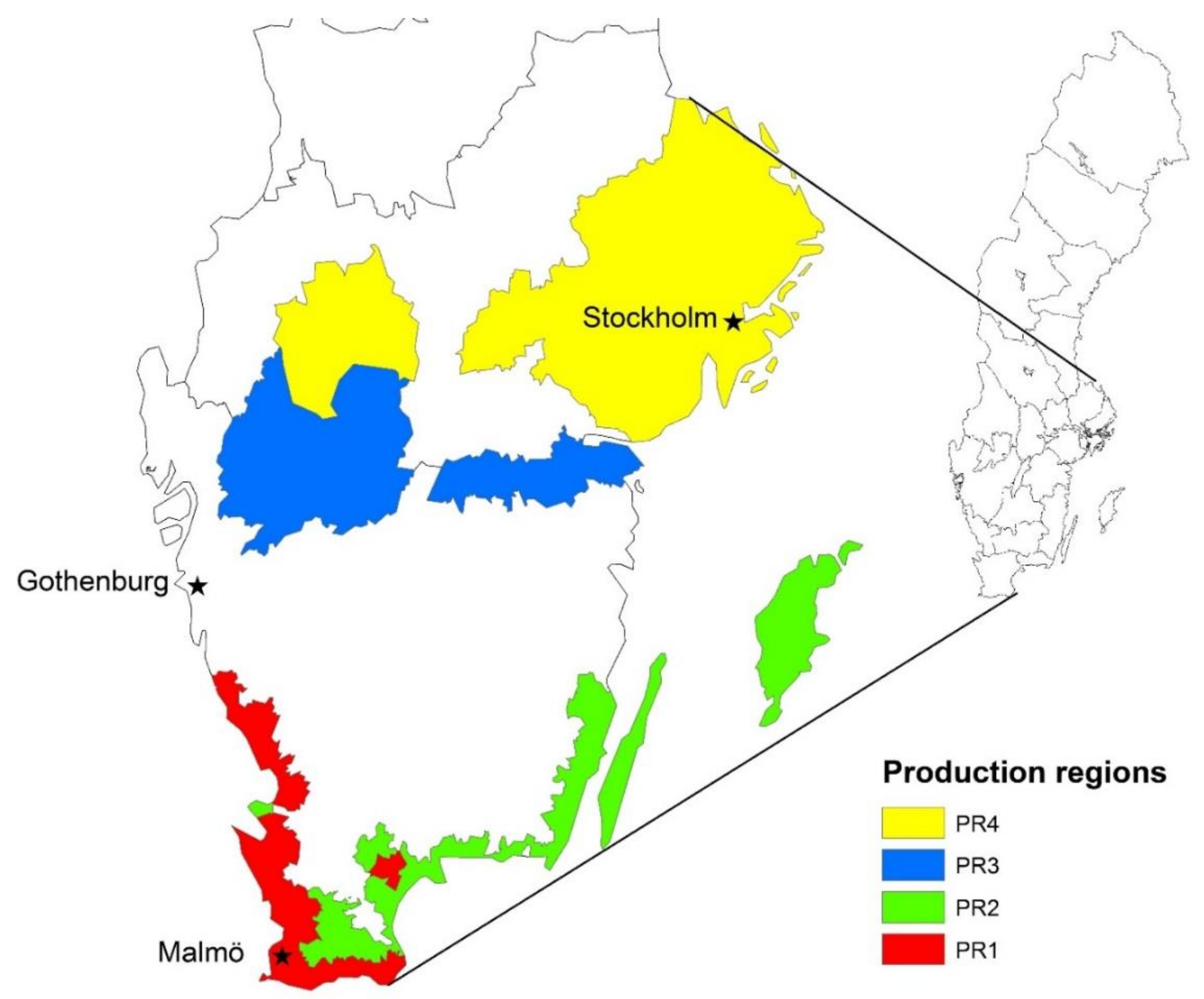
• Inventory and analysis of statistics and data for biomass quantification and the identification of relevant regions and regional differences.
• Inventory and analysis of georeferenced data on soil properties for subsequent simulation of the effects of straw removal on soil organic carbon (SOC) content.
• Assessment of material and product flows in biofuel production using published data on the use of wheat straw and grain for ethanol and biogas production.
• Assessment of GHG emissions according to the ISO (International Organization for standardization) standard for life cycle assessment and by applying the methodology defined in the EU RED.
• Assessment of feedstock production costs using a stepwise calculation method considering field operations, transport and storage.
• Assessment of biogas and ethanol production cost using investment analysis based on the annuity method.

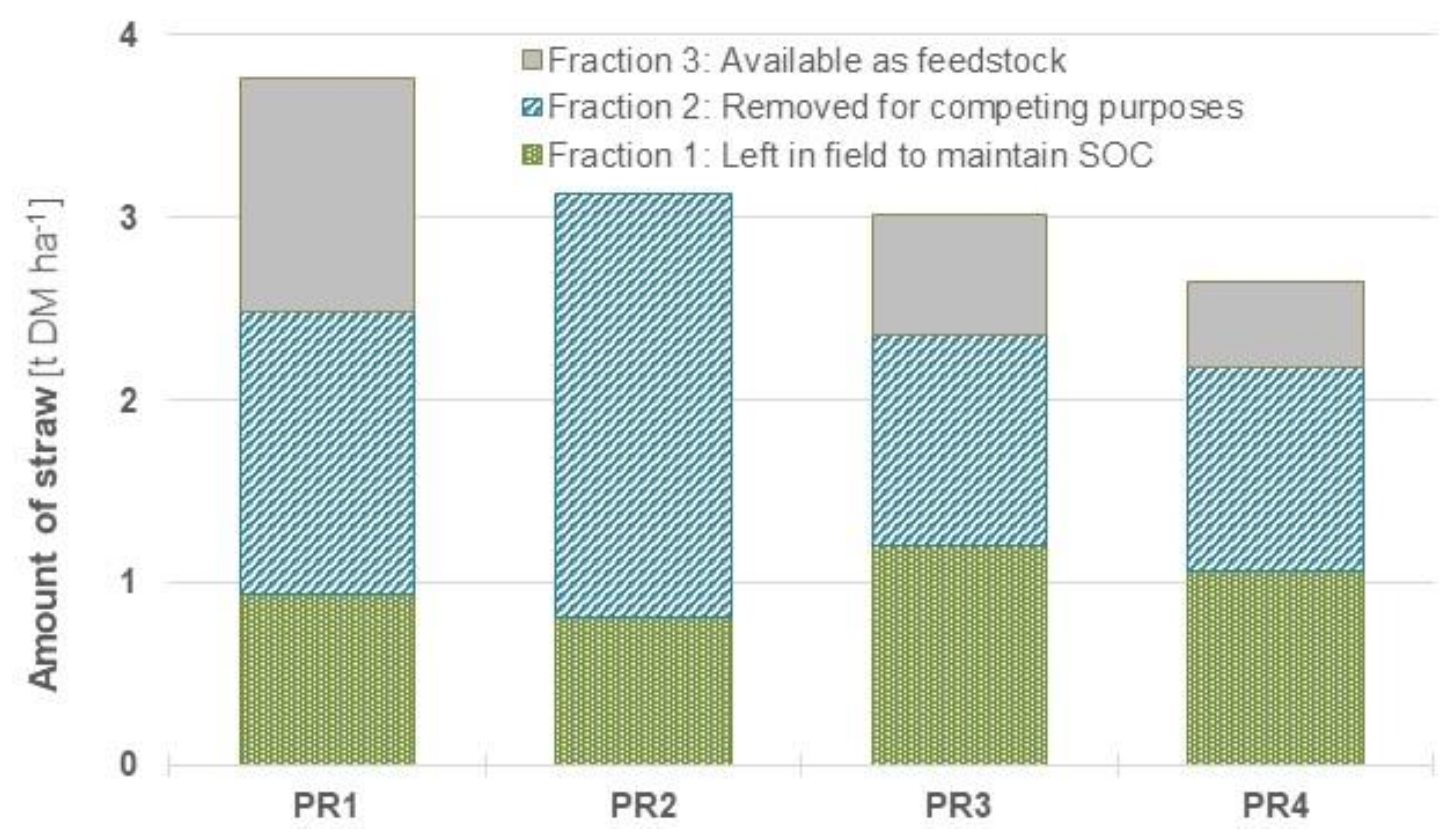
2.1. Feedstock Production and Transport

Sweden is a long, narrow country, extending over 15 degrees of latitude, which means that conditions for the production of cereals and the collection of straw will vary considerably. From an agricultural perspective, Sweden is divided into eight different production regions. In this study we have assessed the four most productive regions (PR1–PR4), each of which is characterised by similar soil type, topography and climate (see Figure 1 and

Table 1. Total area, fraction of arable land and standard yields for winter wheat (2012–2016) in the assessed production regions [14,15,16,17,18].

Production Region	Total Land Area	Arable Land	Fraction of Total Arable Land Sweden	Average Grain Yield	Average Area under Winter Wheat Production
	(ha)	(%)	(%)	(kg DM ha−1)	(ha)
PR1—Gothenland southern plainsslättbygder	552,021	48.5	10.2	6573	93,293
PR2—Gothenland central plains	967,796	30.1	11.1	5468	33,293
PR3—Gothenland northern plains	1,203,550	32.5	14.9	5273	99,177
PR4—Svealands plains	2,963,151	19.5	22.1	4631	90,017

). Together these four regions represent 58% of the arable land in Sweden and 96% of the Swedish winter wheat cultivation area [16]. The winter wheat grain yields used in this study were calculated as 5-year averages based on official statistical sources in the form of standard biomass yields, and varied from 4.6 to 6.6 t dry matter (DM)/ha in the four regions studied (Table 1). For comparison, the average yield of common wheat in 2011–2015 in the EU was 5.0 t DM/ha [17].

Winter wheat straw yields were calculated based on the amount of harvested grain using regional straw/kernel ratios [18]. The amount of straw recovered was assumed to be the total amount of straw minus an unrecoverable stubble of 20 cm. The impact of straw removal on the SOC content was simulated for each of the four production regions based on data on current mean average SOC content, the bulk density of soil and its clay content, and the minimum and maximum SOC content in the production region (see Appendix C). The introductory carbon balance model (ICBM) was used to simulate the amount of SOC lost due to mineralization. The model was calibrated for each production region against data from long-term field experiments. Data on annual yields and SOC content were available for two different crop rotations with 13–16 different fertilization regimes for each field experiment. These data were used to calculate the amounts of residue left on the field. The ICB model was calibrated by adjusting the reaction coefficient for the outflow from the old carbon pool in order to maximize the coefficient of determination of the model predicting the change in SOC content.

The resulting first-year outflow of carbon from the old carbon pool was compared to the amount of carbon added to the old carbon pool from both wheat crop residues left in the field and carbon added as digestate. Wheat crop residues included straw, stubble and root biomass. The fraction of carbon added to the soil expected to enter the old carbon pool was calculated from the amount of carbon added and the humification coefficient (h = 0.15 for straw and stubble; 0.35 for root biomass; 0.27 for digestate) [19]. This is a simplification, since h is the fraction of the annual outflow from the young carbon pool that enters the old carbon pool, resulting in indicative values of stabilized carbon. Also, applying h = 0.15 for calculating the potential negative SOC impacts of straw removal should be seen as a worst case scenario, since straw humification has been suggested to have substantially lower coefficients in more recent studies (h = 0.002 − 0.028 for the PRs studied) [20]. The SOC balance was then calculated by adding the amount of carbon added to the old carbon pool minus the amount of annually mineralized carbon.

Of the total harvestable amount of straw (taking into account weather conditions preventing harvest), three categories were defined that could be used for biofuel production:

• Straw fraction 1, corresponding to the amount of SOC mineralised.
• Straw fraction 2, currently removed and used for other purposes [21].
• Straw fraction 3, available for bioenergy production without having any impact on SOC and without competing with any other uses.

Straw fractions 1, 2 and 3 combined can be regarded as the “technical potential”, and straw fraction 3 as the ecologically or market “restricted potential”. The proportions of each fraction in the different regions vary, depending on local conditions and current use of straw, see Figure 2. In this study, the production cost and GHG emissions were calculated for ethanol and biogas produced from wheat grain and two different amounts of straw removed: (1) The restricted potential including only straw from fraction 3, and (2) the technical potential including straw from fractions 1–3, where straw removal will compete with current use and have a negative impact on SOC content.

The distance over which the feedstock would have to be transported was calculated for each region and biofuel production system, assuming removal of these different fractions of straw. Background data and further assumptions regarding the assessed production system are given in Appendix A.

2.2. Ethanol and Biogas Production and Distribution

Although most of the biofuel used in Sweden is currently imported, there is some domestic commercial-scale production of both ethanol (from grain) and biogas (mainly waste-based) for biofuel applications. Techno-economic data for all production systems were collected from recent studies in which the production of ethanol and biogas from grain or straw had been modelled under Swedish conditions. The scale of production, overall system design and handling of co-products, etc., were chosen so as to be representative of current practice in Sweden.

2.2.1. Ethanol

There is currently one major ethanol production plant in Sweden, with an annual production of approximately 4.9 PJ based on wheat (80%) and barley (20%) grain. Here and in the following sections, energy content is expressed as lower heating value (LHV) for all products. In the present study, mass flow, energy balances and investment costs were based on a model plant producing 4.2 PJ ethanol from 440,000 t DM of grain. In addition to ethanol, it was assumed that the plant also produced distiller’s dried grain with solubles (DDGS), which is dried to 88% DM and used as animal feed [22]. To maximise the biofuel production it is also possible to use the DDGS as feedstock for biogas production. Due to economic reasons this is, however, not practised in Sweden today and therefore not included in this paper.

In the production of ethanol from straw, the location of the plant—so as to ensure a sufficient regional supply of feedstock—has been identified as an important factor for economic feasibility [23]. Production based on an annual straw supply of 120,000 to 200,000 t DM has been considered necessary to give economies of scale in previous Swedish studies [23,24,25,26]. In the present study, calculations are based on an annual straw supply of 200,000 t DM and process performance was optimized by applying high-DM fermentation and organic acid pre-treatment [26].

Most of the DM in cereal grain is starch (based on hexose sugars), while the proportion of hexoses in straw is only about 1/3 of the DM. For straw, ethanol production from hexoses alone has thus been shown to be insufficient to provide economic profitability [26]. Suggested alternatives are the integration of pentose-based fermentation, or the production of biogas in combination with use of the lignin for pellet or combined heat and power production [23,26]. Upgrading of the biogas to vehicle fuel quality has also been shown to have good potential to improve profitability [26]. The solid residue, which is rich in lignin, could also be interesting for further thermochemical conversion. In this study, calculations are based on the fermentation of hexose sugars to ethanol, pellet production from the lignin-rich solid residue after enzymatic hydrolysis, and anaerobic microbial production of methane from the pentose-containing liquid residue after pre-treatment together with the stillage.

The energy required for the distribution of ethanol to filling stations was calculated assuming the use of trucks with a filling capacity of 35 t and an average fuel consumption of 5 kWh per km including empty return transport [27]. The transportation distance was set to 30 km. It was assumed that the biogas was injected into a low-pressure gas grid and distributed to filling stations connected to the grid, which was the case for 40% of the upgraded biogas produced in Sweden in 2016 [28].

Feedstock demand, product yields, additives and energy demand for grain- and straw-based ethanol production are summarized in

Table 2. Material and energy flows in the production of ethanol from wheat grain and straw.

Material and Energy Flows	Grain	Straw	Reference
Feedstock demand (t DM/y)	440,000	200,000	[24,25]
Energy input—process (MWh/t DM)
Natural gas a	1.05		[24]
Wood chips		0.11 b	[27]
Electricity		0.04 c	[27]
Energy input—distribution (MWh/t DM)
Diesel (truck transport)	0.004	0.002	Present work
Electricity (filling station)		0.006	[27]
Additives/Chemicals (kg/t DM)
Acetic acid		1.1	[25]
Ammonia (25%)		40	[25]
Antifoam		0.4	[25]
Enzyme, 1 g	1.1
Enzyme, 2 g		5.6	[25]
H2SO4	7.3		[24]
MgCl2/MgSO4		0.1	[25]
Molasses		26	[25]
NaOH	7.3		[24]
(NH4)2HPO4		1.1	[25]
NH4OH	7.3		[24]
Phosphoric acid		3.5	[25]
Yeast	0.002		[24]
Water	2200	55,900	[26]
Main product (MWh/t DM)
Ethanol	2.67	1.1
Methane		0.8	[24,25]
Co-products (MWh/t DM)
Electricity, incl. internal use	0.25	0.09	[24,25]
Electricity, net output	0.18	0.05	[24,25]
Lignin pellets (at product humidity) d		1.2	[24,25]
DDGS (at product humidity) e	1.55		[24]

^a Used for economic calculations and to calculate GHG emissions in the sensitivity analysis. In the bases case, GHG emissions are calculated based on the use of 1.12 MWh/t DM of wood chips (assuming 85% efficiency instead of 90% for natural gas). ^b Upgrading of biogas. ^c Upgrading and compression of biogas. ^d Corresponds to 206 kg DM/t DM straw. ^e Correspond to 345 kg DM/t DM grain.

. In the case of straw, external energy was required for upgrading of the biogas produced.

2.2.2. Biogas

There are currently 62 plants in Sweden producing biogas of vehicle fuel quality [28]. In 2016, the feedstock at these biogas plants was mainly sewage sludge, manure and various kinds of municipal and industrial organic waste [29]. Although most biogas plants use a mixture of feedstock, the data used in this study are based on a previously published study in which model calculations were applied to plants using grain or straw only [27].

In addition to biogas, the process generates a liquid digestate that contains all the components of the additives and feedstock not converted into biogas (mainly CH₄ and CO₂). In Sweden, 96% of the digestate produced at large-scale co-digestion plants is utilized as biofertilizer on farmland [28]. It is also possible to pelletize the digestate and used it as fertilizer or fuel [29]. This practise is, however, uncommon in Sweden and is therefore not evaluated in this study. When analysing GHG emissions and production cost, we assumed that the biofertilizer would replace conventional mineral fertilizers, taking into account the additional cost and emissions associated with storing and field application compared to mineral fertilizers. The calculated nutrient and carbon contents in digestate are presented in

Table 3. Material and energy flows in the production of biogas from wheat grain and straw [27].

Material and Energy Flows	Grain	Straw
Feedstock demand (t DM/y)	13,100	21,500
Energy input—process (MWh/t DM)
Wood chips	0.48	0.29
Electricity	0.21	0.26
Energy input—distribution (MWh/t DM)
Electricity (filling station)	0.03	0.03
Additives/Chemicals (kg/t DM)
FeSO4	0.03
N		8.69
P		0.25
Trace elements	0.12	0.07
Process water	3200	4200
Main product
Methane (LHV) (MWh/t DM)	3.5	2.1
Co-products
Biofertilizer (kg/t DM)	145	479
whereof
NH4-N	14	8.3
P	5.2	0.6
K	5.5	10
C	108	247

.

In order for biogas to be utilized as a vehicle fuel, CO₂ and various contaminants must be removed by upgrading [30]. The production capacity at existing upgrading plants in Sweden in 2015 varied from 20 to 3450 m³/h, with an average of 600 m³/h [31]. However, from an economic point of view, there is a clear efficiency of scale favouring larger installations. Upgrading technologies also differ regarding their energy and water demand, as well as methane emissions and methane concentration in the upgraded gas [27]. The optimal solution at specific sites is thus determined by local conditions. The feedstock demand, and energy input for biogas systems with a production of 1000 m³/h were calculated based on previous findings and are given in Table 3. As for combined ethanol/biogas production, it was assumed that the biogas was injected into a low-pressure gas grid.

2.3. Economic Assessment

The economic assessment included the production and transport of domestic feedstock to the biofuel production plant, the production and distribution of ethanol and biogas, as well as the production and economic value of co-products such as DDGS, digestate and lignin pellets.

The cost of feedstock production and storage was calculated based on current agricultural practices in Sweden, including, for example, fertilization recommendations. The biofuel production and distribution costs are based mainly on the findings of recent techno-economic studies on biofuel production in Sweden, together with some updated market prices, for example, for process energy. The cost of transportation of feedstock and digestate in biogas production is based on the calculated transportation distance, assumptions on average vehicle speed, and the time required for loading and unloading, as well as hourly rates for different forms of transport carriage. For all economic data, a currency exchange rate of €1 = SEK9.0 was assumed. Further details on the assumptions and background data are given Appendix A and Appendix B.

2.3.1. Capital Cost

The capital cost was calculated based on a weighted average cost of capital (WACC) and depreciation time. The WACC was set to reflect the cost to the producer of acquiring the capital, the expected revenue from alternative investments, and the perceived risk associated with the investment. The depreciation time was set to reflect the anticipated technical life time of the investment, but could also be chosen to reflect the perceived risk, such that high-risk projects are assigned a short depreciation time. Following the assumptions made for ethanol production by Joelsson et al. [22,26] the weighted average cost of capital was set to 11% and the depreciation time was set to 20 years for all investments. In the sensitivity analysis, the WACC was set to 6% and the depreciation time to 15 years, based on the assumptions made in recent calculations of biogas production cost in Sweden [27].

2.3.2. Current Market Price for Vehicle Fuels in Sweden

To evaluate the feasibility of each biofuel system, the calculated production cost was compared with market prices (autumn 2017) for fossil vehicle fuels in Sweden, as presented in

Table 4. Market price (2017) of diesel, petrol and compressed natural gas (CNG) excl. VAT (€/GJ) [32,33,34].

Market Price	Diesel	Petrol	CNG
Fuel price	17.4	17.4	25.5
Energy and CO2 tax	14.3	21.4	6.8
Total price	31.7	38.8	32.3

.

2.4. Greenhouse Gas Emissions

GHG emissions were calculated as global warming potential (GWP) in a 100-year perspective using the EU RED calculation method. The results are expressed per MJ fuel produced, and compared with current GHG reduction criteria and GHG emissions due to iLUC effects [5,8]. The system boundaries were chosen to include the production of raw material up to the point of delivery of biofuel to consumer, and emissions from production were allocated to multiple products based on energy content (LHV at product moisture content). Biofuel feedstocks classified as by-products from other production were set to have zero emission until the point of collection.

In addition, a life cycle assessment was performed based on the approach outlined in the ISO standard [35]. The functional unit was 1 MJ (LHV) of biofuel at the filling station, and the system boundaries were the same as in the EU RED calculations. The main difference of relevance to the present study is that in the ISO method a systems expansion is recommended in the case of multiple products. This includes the assessment of what the co-products are likely to replace, and the resulting benefits in terms of GHG reduction. In addition, the zero-emission approach for by-products applied in the EU RED was replaced by a calculation of the impact of removing the straw from the field. Emphasis was placed on the effects on SOC content, since this is an aspect often discussed in relation to the removal of crop residues. To allow comparison between the results, no other aspects were changed, thus GWP characterization factors and emissions based on typical average emissions were maintained in both assessments. The assumptions and data are summarized in Appendix C.

2.5. Sensitivity Analysis

The uncertainty in the data chosen for material flows, yields and emissions was evaluated from different perspectives depending on the feedstock and process. In addition, the sensitivity of the end result to aspects that can be regulated through policies on EU level, such as the choice of emission factors for electricity, was evaluated for all production systems. The data used in the base case and evaluated alternative values are summarized in

Table 5. Values evaluated in the base case (bold) and alternative values (Further information on the selected emission values and references can be found in Appendix B and Appendix C).

Input—Production	Units	Value	Description
Energy supply—electricity	g CO2eq MJ−1	34.9	Nordic mix
		124	EU28 mix
		13.1	Swedish mix
Energy supply—heat	g CO2eq MJ−1	4.0	Wood chips
		77	EU mix natural gas
Fuel for crop production and transport	g CO2eq MJ−1	80.4	Diesel with low-blend biodiesel
		23.2	Biodiesel
Mineral N manufacture	kg CO2eq kg N−1	4.45	Average use Sweden
		7.8	Western European average
Enzyme dose	g enzyme (100 g cellulose)−1	1.7	Used in techno-economic study
		6.0	Max. trial dose recommended
		6.8	Next-generation enzymes
Enzyme manufacture emissions	kg CO2eq kgenzyme−1	5.5
		8.0
		0.9	Next-generation enzymes
Methane yield—straw	m3 (t DM)−1	224
		202
		247
Straw storage cost	€ (t DM)−1	0.02	Indoor
		0	Outdoor
Capital cost
- Depreciation	years	20
- Depreciation		15
- WACC	%	11
- WACC		6
Investment subsidy	%	0
		30
Co-products
DDGS—sales price	€ (t DM)−1	0.24
		0.34
		0.14
Methane yield (straw ethanol process)	MJ (t DMstraw)−1	2900	Experimentally derived
		6666	Theoretically calculated

. Assumptions, calculations and references are presented in Appendix B (costs) and Appendix C (GWP).

Winter wheat cultivation in four Swedish production regions was evaluated to demonstrate the impact of varying cultivation conditions and transport distances on both production cost and GWP. Other cultivation-related effects evaluated from a GWP perspective were the emissions associated with mineral nitrogen fertilizer production, and the impact of replacing diesel (with a low blend of biodiesel) with biodiesel. Both indoor and outdoor straw storage were evaluated in the cost calculations.

The production of ethanol from grain is a well-established commercial process, and data on yields, both for ethanol and DDGS, and inputs in the process are considered reliable. In the present study, the source of process energy was evaluated, since the typical Swedish conditions assumed in the base case might not be typical in other countries. The type of protein animal feed replaced by DDGS, and the impact of the market value were also evaluated.

When considering straw for ethanol production, the uncertainty in the experimental co-product yield of biogas was taken into consideration by using a low yield in the base case. The impact of a higher yield was also evaluated, which leads to additional processing emissions, and the net impact on GWP and costs is reported in the results. Other aspects evaluated were the enzyme dosage and the GHG emissions resulting from enzyme manufacturing.

Biogas production, upgrading and gas grid injection for vehicle fuel applications are well-established full-scale processes, and the inputs and emissions are considered reliable. However, the yield used here was based on a theoretical calculation and both higher and lower yields were evaluated.

In this study, the investment cost is reflected in the cost of capital, including the depreciation time and the WACC. For ethanol from grain and biogas upgrading and distribution, the investments assumed are considered reliable even if the actual cost is time- and site-dependent. For ethanol from straw, the assumptions are probably more uncertain. In the sensitivity analysis, this was evaluated by changing the depreciation time and the WACC, while keeping the investment cost constant. Finally, the impact of an investment subsidy was also evaluated.

3. Results and Discussion

GHG emissions and production costs were calculated for ethanol and biogas from both wheat grain and wheat straw. The purpose was not only to present updated and comparable values for these biofuel production systems, but also to identify drawbacks and benefits if residues are prioritized over energy crops for the production of biofuels. Based on our base case assumptions, Figure 3 and Figure 4 show production cost and GHG emissions, calculated according to the EU RED and the ISO methodology, for the production of ethanol and biogas from grain and straw originating from PR1. For straw, the results given here include the removal of fraction 3 only (see Section 2.1). To exemplify how reduced GHG emissions could be given an economic value, the results are also applied in the context of the Swedish GHG reduction mandate.

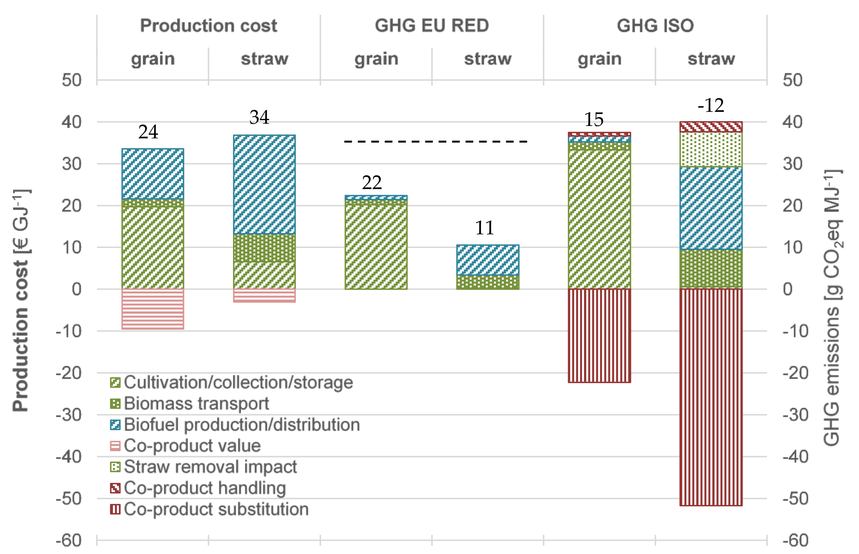
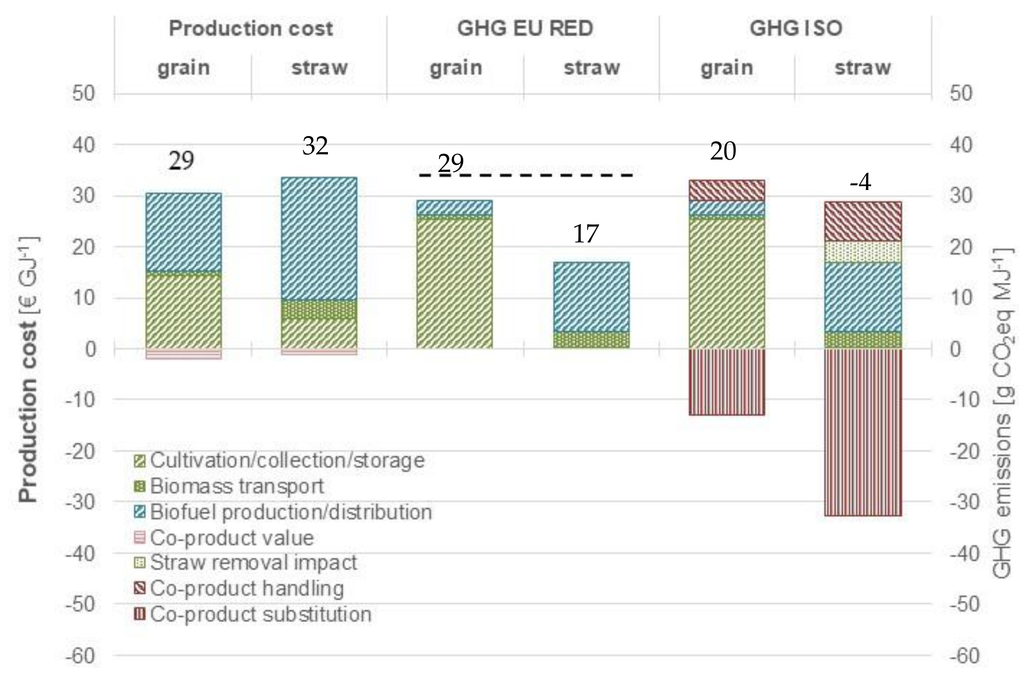
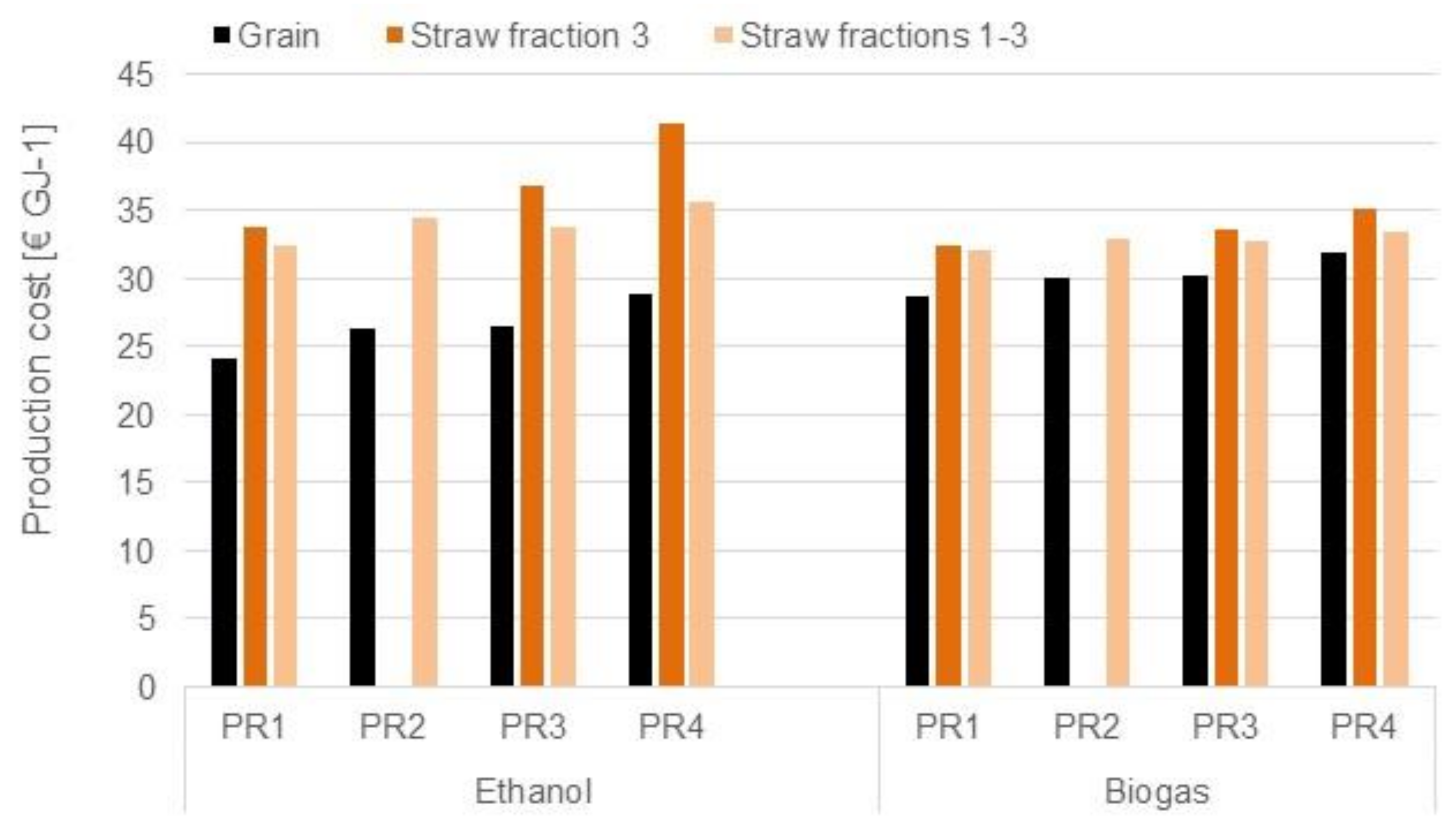
3.1. Production Cost

The production cost for biofuels is calculated to €324–€334/GJ depending on feedstock and fuel, see Figure 3 and Figure 4.

The cost is higher when using straw as feedstock than when using grain. However, the production cost for biofuels based on straw is still lower than the market price of petrol (€39/GJ,) and comparable to the prices of diesel and CNG (€32/GJ) including taxes. It is notable that the cost of grain has a substantial impact on the overall biofuel production cost, while the costs for the collection and storage of straw are not so important and that straw is a cheaper feedstock, even when the transportation cost is included.

The overall production cost is also affected by the economic value of the co-products. This is especially the case when producing ethanol from grain, where the value of the DDGS corresponds to approximately 50% of the biomass cost. Thus, the feasibility of such biofuel production is highly dependent on the market price not only of wheat and biofuel, but also feed such as soybean. It should be noted that the price of straw is not directly affected by the market prices of agricultural commodities. However, the amount of available straw is indirectly affected by the wheat and livestock market, which influence the total amount available and alternative uses of straw.

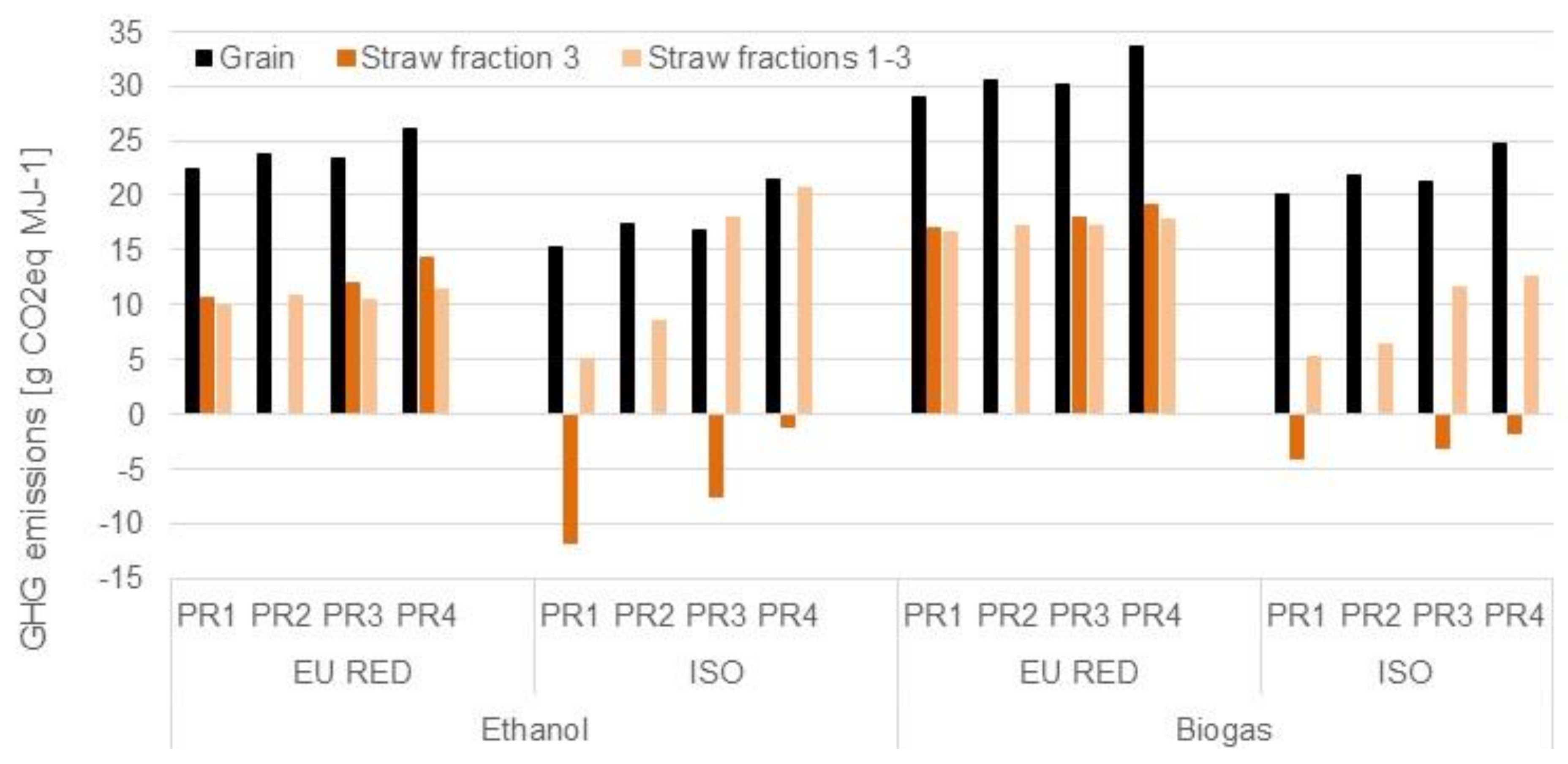
3.2. Greenhouse Gas Emissions

For the production of biofuels from grain, GHG emissions are dominated by biomass production as such. If straw is used, emissions from biomass transport, as well as the biofuel production process, increase, although the total emission is still lower compared to biofuels from grain. The current requirement for biofuels to be considered sustainable in the EU is a 60% reduction of GHG emissions compared to fossil fuels [8]. Both grain- and straw-based biofuels fulfil this requirement, but the reduction is greater for straw-based ethanol and biogas, with savings of 89 and 82%, respectively. In addition, ethanol production from grain has been assigned an iLUC-based GHG emission factor, which is set to 12 g CO₂eq MJ⁻¹ [8]. When this is included, the GHG reduction for grain-based ethanol will decrease to 63%, approaching the limit of what is currently considered sustainable from a GWP perspective.

However, it should be noted that combining GHG emission calculations based on the EU RED methodology with GHG emissions calculated based on an iLUC effect actually constitutes a methodological error. The EU RED is an attributional GHG accounting system for existing specific production chains, while the iLUC is based on economic equilibrium models that estimate the large-scale patterns in global land-use change as an effect of implementing a biofuel policy. Since iLUC factors are implemented in EU biofuel policies, it is however a useful exercise to determine how biofuel producers could be affected.

If GHG emissions are calculated according to the ISO methodology, the net emissions will be lower for all biofuel systems (see Figure 3 and Figure 4). This is mainly due to the emission savings when co-products are included, instead of applying energy-value-based allocation, as in the EU RED. This confirms the climatic advantages of straw-based biofuels, which have the lowest net emissions, irrespective of the method applied.

3.3. Impact of Regional Differences and Ratio of Straw Removal

Results in Figure 3 and Figure 4 were shown for PR1, the region with the most favourable conditions, and with a degree of straw removal that does not affect current utilization or the SOC content. The impact on production costs and emissions of locating a biofuel production plant in regions with lower share of arable land and lower cereal yields (Table 1, PR2–4) was evaluated, together with a higher rate of straw removal (fractions 1–3, see Figure 2).

If a biofuel production plant is located in such a region, the feedstock cost will increase, see Figure 5. When using grain, the overall production cost increases by about 20% for ethanol and 10% for biogas when comparing PR4 with PR1. The majority of the cost increase, 80–90% for ethanol and 90–100% for biogas production, is due to increased crop cultivation cost at lower yields. For straw, the cost increase is solely due to the longer transport distances. The larger ethanol production plant is thus influenced more, with a cost increase of more than 20% in PR4 compared to PR1 when only the currently unutilized straw is used (fraction 3), and 10% when all straw is removed (fractions 1–3). Using straw for ethanol production in PR4 is also the only production system where the biofuel production cost is higher than the market price of petrol (€39/GJ). For biogas production, the impact of changing PR and collecting a higher share of straw is low due to the smaller amounts needed at each plant. If all the straw were to be collected (fractions 1–3), the production cost would be lower than current market prices of petrol in all the production regions investigated.

The same comparison was made for impact on GHG emissions (see Figure 6). Regardless of PR and method of calculation, GHG emissions were lower for biofuels produced from straw than from grain. All systems also exhibited a GHG saving larger than 60%. If an impact of iLUC for grain based ethanol was included, as given in the iLUC directive (12 g CO₂eq MJ⁻¹), a 60% saving in GHG emissions would not be obtained in PR4. For the EU RED calculations, the GHG emissions followed the same pattern as the costs, where lower yields gave the main impact for grain based fuels, and longer transport distances increased the emissions for straw-based fuels.

The ISO calculations showed a more complex picture. As shown in more detail for PR1 in Figure 3 and Figure 4, the different methods applied for handling co-products gave less GHG emissions for grain and straw fraction 3 in all PR. In addition, the ISO calculations included the potential negative impact on SOC when all straw was collected (fractions 1–3). This SOC impact was the main reason to the higher emissions when comparing the use of straw fractions 1–3 to removal of only straw fraction 3, the benefit of the shorter transport distance only having a minor impact. This illustrates how relevant emissions or avoided emission can be missed when the method is as simplified as in the EU RED.

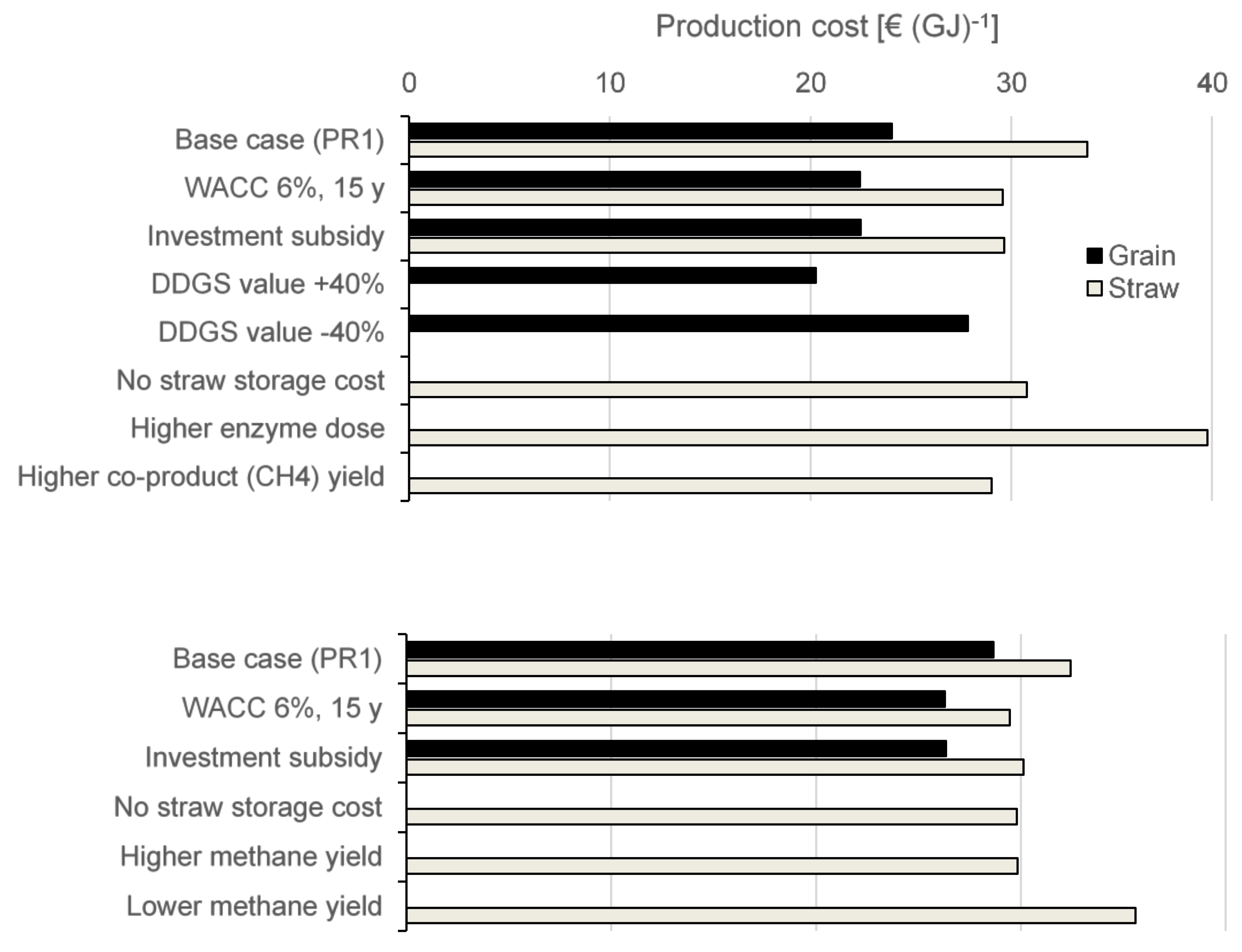
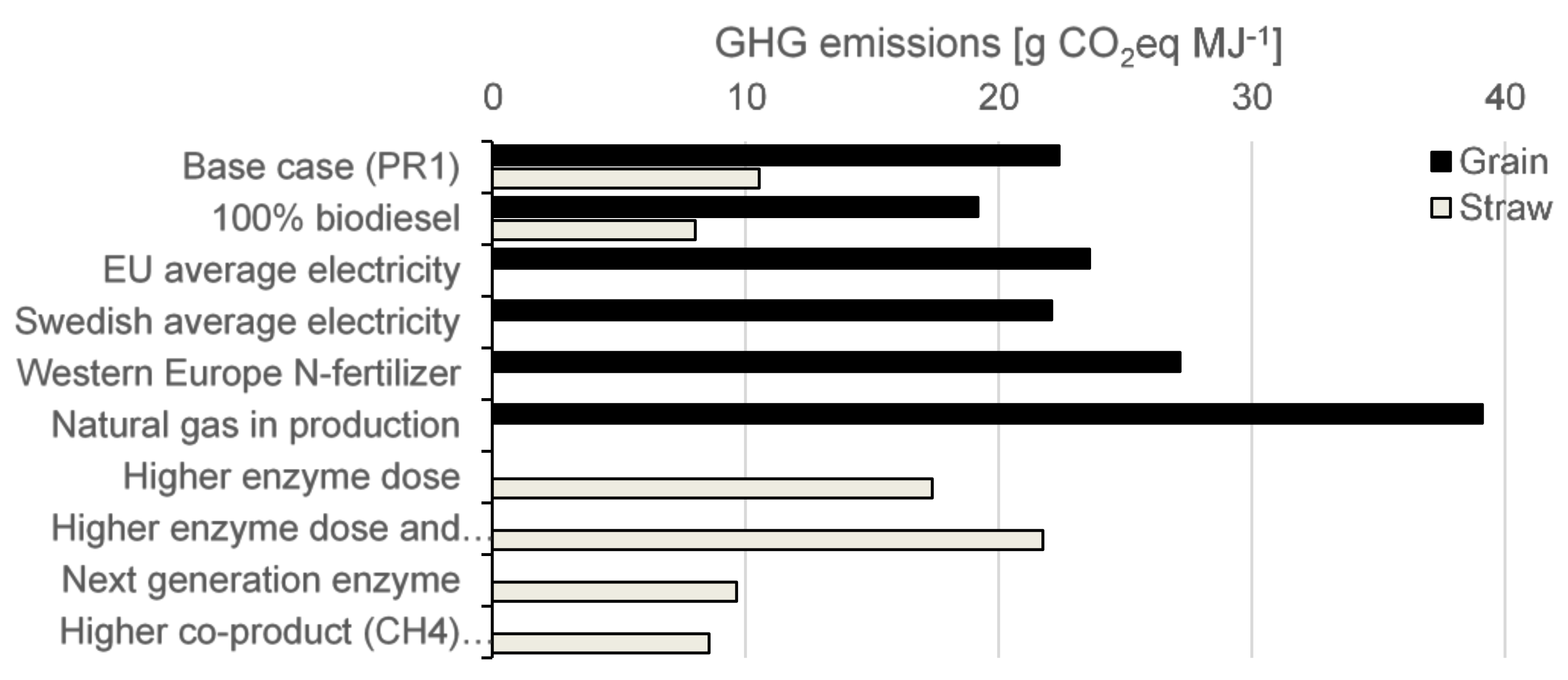
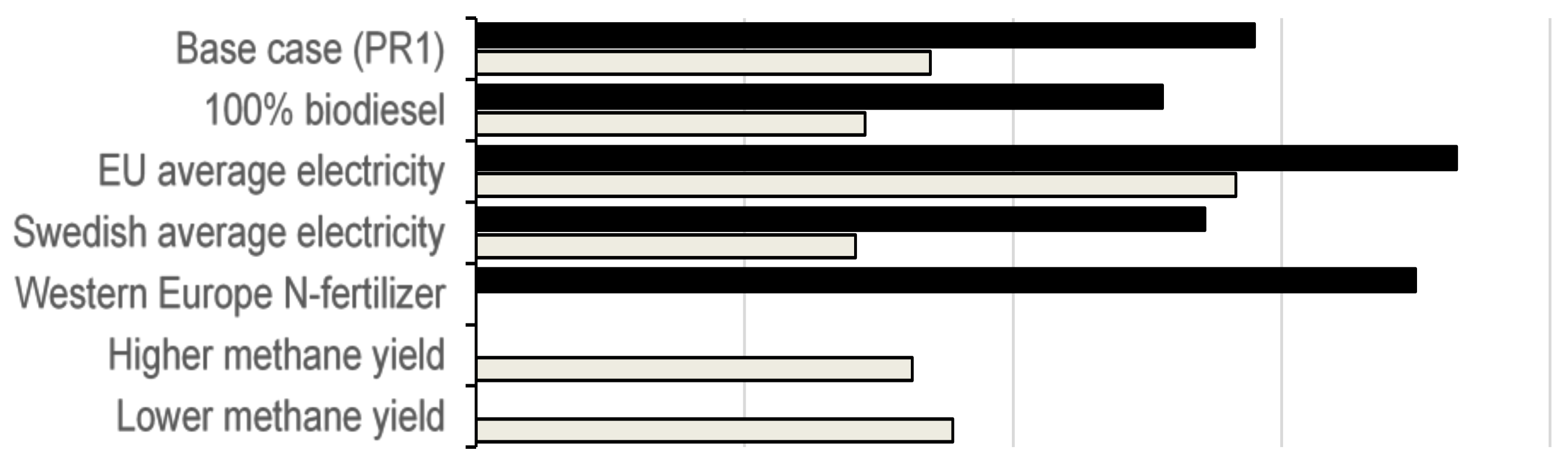
3.4. Sensitivity Analysis

The aspects evaluated in the sensitivity analysis are shown in Figure 7 (production cost) and Figure 8 (GHG emissions according to the EU RED methodology).

As mentioned above, the calculated production cost is lower than the current market price of petrol in all biofuel production systems analysed. The production cost of biofuels from grain is dominated by the cost of the grain. Reducing the interest or the depreciation time, or implementing an investment subsidy would thus have a minor impact on the overall production cost. Although the economic value of the DDGS has a high impact on the ethanol production cost, grain-based ethanol still has the lowest cost even if the market price of DDGS is reduced with 40%.

When straw is used for biofuel production, reducing the capital cost has a greater impact. An investment subsidy of 30%, for example, would lead to a production cost for both biogas and ethanol that is lower than the current market price of all fossil vehicle fuels in Sweden. Finding a cheaper storage solution for straw will also have a positive effect although not dramatic. The ethanol production cost is reduced with approximately 10% if the straw storage cost is set to zero. Finally, it is clear that parameters such as methane yield and enzyme dosage have at least as high an impact as changing the capital cost or the storage cost. Thus, it is crucial to gain a better understanding of these parameters in a full-scale process. However, the production cost only exceeds the current market price of petrol in the case with the highest enzyme dose.

Regarding GHG emissions, the only single factor among those evaluated that increases emissions above the 60% reduction limit is the use of a fossil energy supply, natural gas, in grain-based ethanol production. The emissions for EU average electricity and the typical emission for Western European nitrogen fertilizer also give notable increases in total emissions. Thus, an energy supply based on a high share of renewables and low-emission nitrogen fertilizer production are, not unexpected, aspects that are relevant to low-emission biofuel production. If all diesel used for agricultural operations and transport is replaced with biodiesel (here 50% FAME and 50% HVO, see Appendix C), this would also give a significant reduction of GHG emissions. For straw-based biofuels, methane yield, enzyme dose and GHG emissions from enzyme production have impact on overall emissions. However, the parameters evaluated here do not risk the possibility of achieving a GHG saving of 60% or higher.

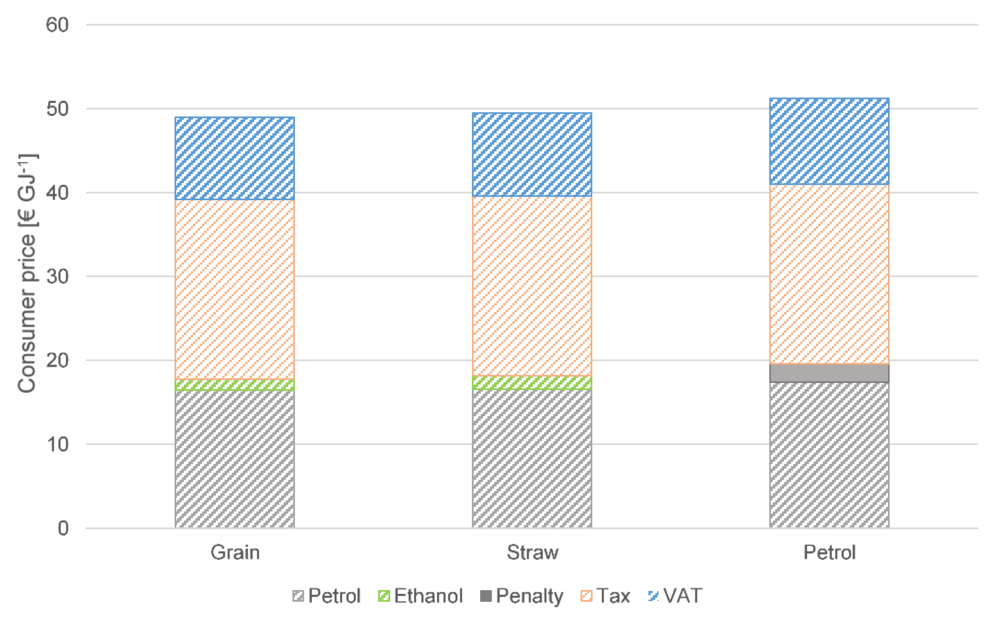
3.5. Ethanol from Grain vs. Straw with a GHG Reduction Mandate

As presented in the introduction, Sweden has implemented a system with a GHG reduction mandate for low-blend of biofuels in petrol and diesel. With this system, the amount of biofuel required depend on its GHG reduction. A biofuel with low emissions will thus have a higher value than a biofuel with higher emissions. The calculated consumer price for petrol, including the mandatory low-blend of ethanol in 2020 (4.2%) is presented in Figure 9. The amount of ethanol required is based on the GHG emission calculated according to the EU RED and the cost is based on the result presented in Figure 3. Even with the advantage given by the reduction mandate system, ethanol from straw is still the more expensive option. However, the overall cost of the fuel blend will only increase by approximately 1% if the fuel supplier chooses ethanol made from straw instead of grain. As can be seen in Figure 9, using ethanol produced from straw is also cheaper than paying the penalty for not fulfilling the reduction mandate.

4. Conclusions

Wheat grain and straw are two examples of agricultural feedstocks that could be used to produce biofuels such as biogas and ethanol. The results of this study clearly shows that straw-based production gives biofuels with lower GHG emissions, regardless of the calculation method applied. From an economic perspective, the production cost for biofuels from both grain and straw are lower or similar to the market price of fossil fuels. The production of biofuels from grain is far less costly, despite the fact that the cost of the feedstock is higher than that of straw. Thus, there is a trade-off between cost and climate impact in these studied comparisons of biofuels from the grain and the straw from wheat.

In this study, climate impact has been calculated according to the method given in the EU RED, which is applied in the currently implemented European biofuel policies, as well as according to the ISO standard for LCA. Biofuels from straw were found to have the lowest climate impact regardless of calculation method. The method in the EU RED is, however, simplified and does not include the whole biofuel production system. Thus, there is a risk that relevant emissions or avoided emission is excluded and that implemented policy instruments does not favour the biofuels with the lowest GHG emissions. To avoid this, the method applied in the EU RED should be modified so that co-products and changes in SOC is fully included for all biofuels and feedstock.

In a Swedish context, the production of biogas and ethanol from both grain and straw fulfils current demands on GHG emission reductions in the EU RED. In fact, the production of biofuels from grain could still meet the reduction requirements even including the iLUC-factors suggested in the amended EU RED. This would, however, demand a production system characterized by a high share of renewable energy carriers (both in transport and production), and the use of mineral fertilizers produced with low GHG emissions.

The reduction mandate recently adopted in Sweden is used as an example of policy implications of the observed trade-off between climate impact and cost. Such a system increases the competitiveness of ethanol from straw over grain, but does not compensate completely for the higher production cost. Fuel suppliers are thus likely to use as much biofuels from crops as is permitted by current policy instruments. However, producing ethanol from straw instead of grain would have only a minor impact on the fuel price to the consumer. Thus, if there is a shortage of ethanol from grain, or policy instruments limit the use of this feedstock, producing ethanol from straw is a highly viable option.

References

1. European Commission (EC). Communication from the Commission to the European Parliament, the Council, the European Economic and Social Committee and the Committee of the Regions—A Policy Framework for Climate and Energy in the Period from 2020 to 2030; COM (2014) 15 Final; European Commission: Brussels, Belgium, 2014. [Google Scholar]
2. European Environment Agency (EEA). Key Trends and Drivers in Greenhouse Gas Emissions in the EU in 2015 and Over the Past 25 Years; European Environment Agency: Copenhagen, Denmark, 2017. [Google Scholar]
3. The Government of Sweden. The Climate Policy Framework. Available online: http://www.government.se/articles/2017/06/the-climate-policy-framework/ (accessed on 29 September 2018).
4. Trafikverket. Åtgärder för att Minska Transportsektorns Utsläpp av Växthusgaser—Ett Regeringsuppdrag; Trafikverket 2016:111; Trafikverket: Boren, Sweden, 2016. [Google Scholar]
5. European Union (EU). Directive 2009/28/EC of the european parliament and of the council of 23 April 2009 on the promotion of the use of energy from renewable sources and amending and subsequently repealing Directives 2001/77/EC and 2003/30/EC. Off. J. Eur. Union 2009, L140, 16–62. [Google Scholar]
6. Eurostat. Share of Renewable Energy in Fuel Consumption of Transport. Available online: http://ec.europa.eu/eurostat/web/products-datasets/-/tsdcc340 (accessed on 1 November 2017).
7. Energimyndigheten. Drivmedel 2016 Mängder, Komponenter och Ursprung Rapporterade Enligt Drivmedelslagen och Hållbarhetslagen; ER 2017:12; Energimyndigheten: Eskilstuna, Sweden, 2017. [Google Scholar]
8. European Union (EU). Directive (EU) 2015/1513 of the European Parliament and of the Council of 9 September 2015 Amending Directive 98/70/EC Relating to the Quality of Petrol and Diesel Fuels and Amending Directive 2009/28/EC on the Promotion of the Use of Energy from Renewable Sources; European Union: Brussels, Belgium, 2015. [Google Scholar]
9. Ahlgren, S.; Di Lucia, L. Indirect land use changes of biofuel production—A review of modelling efforts and policy developments in the European Union. Biotechnol. Biofuels 2014, 7, 10. [Google Scholar] [CrossRef] [PubMed]
10. Popp, J.; Kot, S.; Lakner, Z.; Oláh, J. Biofuel use: Peculiarities and implications. J. Secur. Sustain. Issues 2018, 7, 477–493. [Google Scholar] [CrossRef]
11. De Rosa, M.; Knudsen, M.T.; Hermansen, J.E. A comparison of Land Use Change models: Challenges and future developments. J. Clean. Prod. 2016, 113, 183–193. [Google Scholar] [CrossRef]
12. Ahlgren, S.; Björnsson, L.; Prade, T.; Lantz, M. Biofuels from Agricultural Biomass—Land Use Change in a Swedish Perspective; 2017:13; f3 The Swedish Knowledge Centre for Renewable Transportation Fuels: Göteborg, Sweden, 2017. [Google Scholar]
13. Tonini, D.; Hamelin, L.; Astrup, T.F. Environmental implications of the use of agro-industrial residues for biorefineries: Application of a deterministic model for indirect land-use changes. Glob. Chang. Boil. Bioenergy 2016, 8, 690–706. [Google Scholar] [CrossRef] [Green Version]
14. Prade, T.; Björnsson, L.; Lantz, M.; Ahlgren, S. Can domestic production of iLUC-free feedstock from arable land supply Sweden’s future demand for biofuels? J. Land Use Sci. 2017, 12, 407–441. [Google Scholar] [CrossRef] [Green Version]
15. Svensk Författningssamling (SFS). Lag (2017:1201) om Reduktion av Växthusgasutsläpp Genom Inblandning av Biodrivmedel i Bensin och Dieselbränslen; The Swedish Code of Statutes, Uppdaterad t.o.m. SFS 2017:1233; Svensk Författningssamling: Stockholm, Sweden, 2017. [Google Scholar]
16. Larsson, S. Sveriges Jordbruksområden—En Redovisning av Jordbruksområden och Växtzoner i Svenskt Jord- och Trädgårdsbruk; Field Research Unit, Swedish University of Agriculutural Sciences: Uppsala, Sweden, 2004; p. 13. [Google Scholar]
17. European Commission (EC). Agriculture in the European Union—Market Statistical Information; European Commission: Brussels, Belgium, 2014. [Google Scholar]
18. Henriksson, A.; Stridsberg, S. Möjligheter att Använda Halmeldning Till Energiförsörjningen i Södra SVERIGE; Department of Agricultural Engineering, Swedish University of Agricultural Sciences: Uppsala, Sweden, 1992. [Google Scholar]
19. Kätterer, T.; Bolinder, M.A.; Andrén, O.; Kirchmann, H.; Menichetti, L. Roots contribute more to refractory soil organic matter than above-ground crop residues, as revealed by a long-term field experiment. Agric. Ecosyst. Environ. 2011, 141, 184–192. [Google Scholar] [CrossRef] [Green Version]
20. Poeplau, C.; Kätterer, T.; Bolinder, M.A.; Börjesson, G.; Berti, A.; Lugato, E. Low stabilization of aboveground crop residue carbon in sandy soils of Swedish long-term experiments. Geoderma 2015, 237–238, 246–255. [Google Scholar] [CrossRef]
21. Statistiska Centralbyrån (SCB). Odlingsåtgärder i Jordbruket 2012. Träda, Slåttervall, vårkorn, Höstspannmål samt Användning av Halm och Blast; Statistics Sweden: Stockholm, Sweden, 2013; p. 44.
22. Joelsson, E.; Borbála, E.; Galbe, M.; Wallberg, O. Techno-economic evaluation of integrated first- and second generation ethanol production from grain and straw. Biotechnol. Biofuels 2016, 9. [Google Scholar] [CrossRef] [PubMed]
23. Ekman, A.; Wallberg, O.; Joelsson, E.; Börjesson, P. Possibilities for sustainable biorefineries based on agricultural residues—A case study of potential straw-based ethanol production in Sweden. Appl. Energy 2013, 102. [Google Scholar] [CrossRef]
24. Karlsson, H.; Börjesson, P.; Hansson, P.-A.; Ahlgren, S. Ethanol production in biorefineries using lignocellulosic feedstock—GHG performance, energy balance and implications of life cycle calculation methodology. J. Clean. Prod. 2014, 83, 420–427. [Google Scholar] [CrossRef]
25. Pål, B.; Ahlgren, S.; Barta, Z.; Björnsson, L.; Ekman, A.; Erlandssson, P.; Hansson, P.-A.; Hanna, K.; Kreuger, E.; Lindstedt, J.; et al. Sustainable Performance of Lignocellulose-Based Ethanol and Biogas Co-Produced in Innovative Biorefinery Systems; Environmental and Energy System Studies, LTH: Lund, Sweden, 2013. [Google Scholar]
26. Joelsson, E.; Dienes, D.; Kovacs, K.; Galbe, M.; Wallberg, O. Combined production of biogas and ethanoil at high solids loading from wheat straw impegrenated with acetic acid: Experimental study and techno-economic evaluation. Sustain. Chem. Process. 2016, 4, 14. [Google Scholar] [CrossRef]
27. Lantz, M.; Kreuger, E.; Björnsson, B. An economic comparison of dedicated crops vs agricultural residues as feedstock for biogas of vehicle fuel quality. AIMS Energy 2017, 5, 28. [Google Scholar] [CrossRef]
28. Energimyndigheten. Produktion och Användning av Biogas och Rötrester år 2016; ES 2017:07; Energimyndigheten: Eskilstuna, Sweden, 2017. [Google Scholar]
29. Lantz, M. Hållbarhetskriterier för Biogas—En Översyn av Data och Metoder; Report 100; Environmental and Energy System Studies, Lund University: Lund, Sweden, 2017. [Google Scholar]
30. Petersson, A.; Wellinger, A. Biogas Upgrading Technologies—Development and Innovations; IEA Bioenergy Task 37; European Commission Joint Research Centre: Petten, The Netherlands, 2009. [Google Scholar]
31. International Energy Agency (IEA). Biogas Upgrading Plant List, Data Up to the End of 2015; IEA Bioenergy Task 37; European Commission Joint Research Centre: Petten, The Netherlands, 2016. [Google Scholar]
32. Svenska Petroleum och Biodrivmedel Institutet (SPBI). Priser och skatter [Prices and Taxes]. Available online: http://spbi.se/statistik/priser/ (accessed on 17 November 2017).
33. CircleK. Drivmedelspriser för privatkunder [Vehicle Fuel Prices]. Available online: https://www.circlek.se/sv_SE/pg1334072467111/privat/drivmedel/Priser/Priser-privatkund.html (accessed on 17 November 2017).
34. Skatteverket. Skattesatser på Bränslen Och el 2017 [Tax on Fuel and Electricity 2017]. Available online: https://www.skatteverket.se/foretagochorganisationer/skatter/punktskatter/energiskatter/skattesatser.4.77dbcb041438070e0395e96.html (accessed on 17 November 2017).
35. International Organization for Standardization (ISO). ISO 14044:2006. Environmental Management—Life Cycle Assessment—Requirements and Guidelines; ISO: Geneva, Switzerland, 2006. [Google Scholar]
36. Hansson, P.; Saltzman, I.-L.; Bååth Jacobsson, S.; Petersson, P. Produktionsgrenskalkyler för Växtodling—Efterkalkyler för år 2014—Södra Sverige; Hushållningssällskapen Kalmar-Kronoberg-Blekinge, Krisitanstad, Malmöhus och Halland: Kalmar, Sweden, 2014; p. 62. [Google Scholar]
37. Green, M.B. Energy in pesticide manufacture, distribution and use. In Energy in Plant Nutrition and Pest Control; Helsel, Z.R., Ed.; Elsevier: New York, NY, USA, 1987; Volume 2, pp. 165–178. [Google Scholar]
38. BCS. Chapter 9—Limestone and crushed rock. In Energy and Environmental Profil of the U.S. Mining Industry; U.S. Department of Energy, Office of Energy Efficiency and Renewable Energy: Washington, DC, USA, 2002; p. 12. [Google Scholar]
39. Statens Jordbruksverk (SJV). Riktlinjer för Gödsling och Kalkning 2017; Swedish Board of Agriculture: Jönköping, Sweden, 2016; p. 100.
40. Statens Jordbruksverk (SJV). Jordbruksverkets Produktlista. Available online: http://www.jordbruksverket.se/download/18.773c089e128e1620fa5800087307/1370041066727/Produktlista100610.pdf (accessed on 8 August 2014).
41. Engquist, M.; Jansson, S.; Johansson, C.; Algerbo, P.-A.; Johnson, F.; Neuman, L. Maskinkostnader 2016; LRF Konsult: Linköping, Sweden, 2016; p. 48. [Google Scholar]
42. Berglund, M.; Börjesson, P. Assessment of energy performance in the life-cycle of biogas production. Biomass Bioenergy 2006, 30, 254–266. [Google Scholar] [CrossRef]
43. Börjesson, P. Energianalyser av Biobränsleproduktion i Svenskt Jord- och Skogsbruk - idag och kring 2015; Department of Technology and Society, Lund University: Lund, Sweden, 1994; p. 67. [Google Scholar]
44. Overend, R.P. The Average Haul Distance and Transportation Work Factors for Biomass Delivered to a Central Plant. Biomass 1982, 2, 75–79. [Google Scholar] [CrossRef]
45. Börjesson, P.; Gustavsson, L. Regional production and utilization of biomass in Sweden. Energy 1996, 21, 747–764. [Google Scholar] [CrossRef]
46. HIR Maskinkostnader 2016; Swedish Rural Economy and Agricultural Societies: Bjärred, Sweden, 2016.
47. Statistiska Centralbyrån (SCB). Energipriser på Naturgas och el [Energy Prices for Natural Gas and Electricity]. Available online: http://www.scb.se/EN0302 (accessed on 23 September 2017).
48. Rosenqvist, H. Kalkyler för Energigrödor 2017—Fastbränsle, Biogas, Spannmål och Raps; Jordbruksverket: Jönköping, Sweden, 2017. [Google Scholar]
49. Seider, W.D.; Seader, J.D.; Lewin, D.R.; Widagdo, S. Product and Process Design Principles-Synthesis, Analysis, and Evaluation; Wiley: Hoboken, NJ, USA, 2010. [Google Scholar]
50. Lantz, M.; Björnsson, L. Biogas från Gödsel och Vall—Analys av Föreslagna Styrmedel; LRF—The Federation of Swedish Farmers: Stockholm, Sweden, 2011. [Google Scholar]
51. Börjesson, P.; Lantz, M.; Andersson, J.; Björnsson, L.; Fredriksson Möller, B.; Fröberg, M.; Hanarp, P.; Hulteberg, C.; Iverfeldt, E.; Lundgren, J.; et al. Methane as Vehicle Fuel—A Well-to-Wheel Analysis (Metdriv); Report 2016:06; f3 The Swedish Knowledge Centre for Renewable Transportation Fuels: Göteborg, Sweden, 2016. [Google Scholar]
52. Energimyndigheten. Övervakningsrapport Avseende Skattefbefrielse för Flytande Biodrivmedel under 2016; Energimyndigheten: Eskilstuna, Sweden, 2017. [Google Scholar]
53. Agriwise. Områdeskalkyler 2017—lagring av spannmål. 2017, Database for economic planning and analysis, Swedish Agricultural University. Available online: www.agriwise.org (accessed on 23 September 2017).
54. Biggs, C.; Edward, O.; Valin, H.; Peters, D.; Spoettle, M. Decomposing Biofuel Feedstock Crops and Estimating Their ILUC Effects; Ecofys: Utrecht, The Netherlands, 2016. [Google Scholar]
55. Nordpool. System Price. Available online: http://www.nordpoolspot.com/Market-data1/Dayahead/Area-Prices/SYS1/Yearly/?view=table (accessed on 28 December 2017).
56. Energimyndigheten. En Svensk-Norsk Elcertificatsmarknad—Årsrapport för 2016; Report ET 2017:9; Energimyndigheten and Norges Vassdrag- och Energidirektorat: Eskilstuna, Sweden, 2017. [Google Scholar]
57. Statistiska Centralbyrån (SCB). Trädbränsle och torvpriser nr 3 2017, Sveriges Officiella Statistik; EN 0307 SM 1703; Statistics Sweden: Stockholm, Sweden, 2017.
58. Intergovernmental Panel on Climate Change (IPCC). IPCC Guidelines for National Greenhouse Gas Inventories; Eggleston, S., Buendia, L., Miwa, K., Ngara, T., Tanabe, K., Eds.; Prepared by the National Greenhouse Gas Inventories Programme; The Intergovernmental Panel on Climate Change, Institute for Global Environmental Strategies: Kamiyamaguchi Hayama, Japan, 2006; Volume 4. [Google Scholar]
59. Energimyndigheten. Drivmedel 2016; The Swedish Energy Agency: Eskilstuna, Sweden, 2017. [Google Scholar]
60. Energimyndigheten. Vägledning Till Regelverket om Hållbarhetskriterier för Biodrivledel och Flytande Biobränslen; The Swedish Energy Agency: Eskilstuna, Sweden, 2012. [Google Scholar]
61. Moro, A.; Lonza, L. Electricity carbon intensity in European Member States: Impacts on GHG emissions of electric vehicles. Transp. Res. Part D Transp. Environ. 2017. [Google Scholar] [CrossRef]
62. Börjesson, P.; Tufvesson, L.; Lantz, M. Livscykelanalys av Svenska Biodrivmedel; Environmental and Energy Systems Studies, Lund University: Lund, Sweden, 2010; pp. 1102–3651. [Google Scholar]
63. Edwards, R.; Larive, J.-E.; Rickeard, D.; Weindorf, W. Well to tank Appendix 2—Version 4a Summary of Energy and GHG Balance of Individual Pathways; Joint Research Center, Institute for Energy and Transport: Ispra, Italy, 2014. [Google Scholar]
64. Fossum, J.P. Calculation of Carbon Footprint of Fertilizer Production; Yara HESQ: Oslo, Norway, 2014. [Google Scholar]
65. Biograce. Biograce Version 4d 2015 ed. 2015. Available online: http://www.biograce.net/home (accessed on 29 September 2018).
66. Kool, A.; Marinussen, M.; Blonk, H. LCI Data for the Calculation Tool -Feedprint for Greenhouse Gas Emissions of Feed Production and Utilization GHG EMISSIONS of N, P and K Fertilizer Production; Blonk Consultants: Gouda, The Netherlands, 2012. [Google Scholar]
67. Ahlgren, S.; Röös, E.; Di Lucia, L.; Sundberg, C.; Hansson, P.-A. EU sustainability criteria for biofuels: Uncertainties in GHG emissions from cultivation. Biofuels 2012, 3, 399–411. [Google Scholar] [CrossRef]
68. Statistiska Centralbyrån (SCB). Statistics Sweden Database. Varuimport från Avsändningsland, ej Bortfallsjusterat, ton efter Handelspartner, varugrupp SITC och år, 5621 Mineral or Chemical Fertilizers, Nitrogenous, 2016; Statistics Sweden: Örebro, Sverige, 2017.
69. Adom, F.; Dunn, J. Material and Energy Flows in the Production of Macro and Micronutrients, Buffers, and Chemicals used in Biochemical Processes for the Production of Fuels and Chemicals from Biomass; Argonne National Laboratory: Argonne, IL, USA, 2015. [Google Scholar]
70. Olofsson, J.; Barta, Z.; Börjesson, P.; Wallberg, O. Integrating enzyme fermentation in lignocellulosic ethanol production: life-cycle assessment and techno-economic analysis. Biotechnol. Biofuels 2017, 10, 51. [Google Scholar] [CrossRef] [PubMed]
71. Novozymes. Novozymes Cellic® CTec3 Application Sheet; Novozymes A/S: Bagsvaerd, Denmark, 2012. [Google Scholar]
72. Karlsson, H.; Ahlgren, S.; Sandgren, M.; Passoth, V.; Wallberg, O.; Hansson, P.-A. Greenhouse gas performance of biochemical biodiesel production from straw: Soil organic carbon changes and time‑dependent climate impact. Biotechnol. Biofuels 2017, 10, 2017. [Google Scholar] [CrossRef] [PubMed]
73. Jordbruksverket. Marknadsöversikt-Vegetabilier; The Swedish Board of Agriculture: Jönköping, Sweden, 2012. [Google Scholar]
74. Flysjö, A.; Cederberg, C.; Strid, I. LCA-Databas för Konventionella Fodermedel; SIK Rapport; SIK Institutet för Livsmedel och Bioteknik: Göteborg, Sweden, 2008. [Google Scholar]
75. Björnsson, L.; Prade, T.; Lantz, M. Grass for Biogas-Arable Land as Carbon Sink. An Environmental and Economic Assessment of Carbon Sequestration in Arable Land through Introduction of Grass for Biogas Production; Energiforsk: Stockholm/Malmö, Sweden, 2016. [Google Scholar]
76. Swedish environmental Protection Agency (SEPA). National Inventory Report Sweden 2015. Greenhouse Gas Emission Inventiories 1999–2013; Swedish Environmental Protection Agency: Stockholm, Sweden, 2015.
77. Karlsson, S.; Rodhe, L. Översyn av Statistiska Centralbyråns Beräkning av Ammoniakavgången i Jordbruket—Emissionsfaktorer för Ammoniak vid Lagring och Spridning av Stallgödsel; JTI—Institutet för Jordbruks- och Miljöteknik: Uppsala, Sweden, 2002. [Google Scholar]
78. Carlsson, C.; Kyllmar, K.; Ulén, B. Typområden på Jordbruksmark—Växtnäringsförluster i små Jordbruksdominerade Avriningsområden 2001/2002; Division of water Quality Management, Swedish University of Agricultural Sciences: Uppsala, Sweden, 2003. [Google Scholar]
79. Andren, O.; Katterer, T. ICBM: The introductory carbon balance model for exploration of soil carbon balances. Ecol. Appl. 1997, 7, 1226–1236. [Google Scholar] [CrossRef]
80. Kungl. Skogs- och Lantbruksakademiens (KSLA). Success Stories of Agricultural Long-term Experiments; Åke Barklund, General Secretary and Managing Director; KSLA: Stockholm, Sweden, 2007; p. 108. [Google Scholar]
81. Petersen, J.; Mattsson, L.; Riley, H.; Salo, T.; Thorvaldsson, G.; Christensen, B.T. Long Continued Agricultural Soil Experiments: Nordic Research Platform—A Catalog; Norden: Hellerup, Denmark, 2008; p. 103. [Google Scholar]
Figure 1. Map showing the four most productive agricultural regions in Sweden.
Energies 11 02633 g001
Figure 2. Distribution of straw fractions in the assessment of the different production regions (PR1–PR4).
Energies 11 02633 g002
Figure 3. Production cost and emissions for ethanol produced in PR1 calculated according to the methods in the EU RED and the ISO standard. The dotted line indicates maximum GHG emissions for new installations according to the EU RED. Numbers above the columns indicate net value.
Energies 11 02633 g003
Figure 4. Production cost and emissions for biogas produced in PR1 calculated according to the methods in the EU RED and the ISO standard. The dotted line indicates maximum GHG emissions for new installations according to the EU RED. Numbers above the columns indicate net value.
Energies 11 02633 g004
Figure 5. Cost impact of regional differences and ratio of straw removal. PR2 has no available straw in fraction 3.
Energies 11 02633 g005
Figure 6. GHG emission impact of regional differences and ratio of straw removal. The outcome using two calculation methods (EU RED and ISO) is compared. PR2 has no available straw in fraction 3.
Energies 11 02633 g006
Figure 7. Results of the sensitivity analysis on the production costs for various ethanol (above) and biogas (below) production systems.
Energies 11 02633 g007
Figure 8. Results of the sensitivity analysis on GWP for various ethanol (above) and biogas (below) production systems.
Energies 11 02633 g008aEnergies 11 02633 g008b
Figure 9. Consumer price for petrol including low-blend of ethanol from grain or straw based on the Swedish low blend reduction mandate for 2020.
Energies 11 02633 g009