Abstract
A maximum power point tracker (MPPT) should be designed to deal with various weather conditions, which are different from region to region. Customization is an important step for achieving the highest solar energy harvest. The latest development of modern machine learning provides the possibility to classify the weather types automatically and, consequently, assist localized MPPT design. In this study, a localized MPPT algorithm is developed, which is supported by a supervised weather-type classification system. Two classical machine learning technologies are employed and compared, namely, the support vector machine (SVM) and extreme learning machine (ELM). The simulation results show the outperformance of the proposed method in comparison with the traditional MPPT design.
1. Introduction
A photovoltaic (PV) system, which generates electric power purely from solar energy is an important solution towards future-generation smart grid planning, pollution reduction and sustainable global energy saving [1,2,3]. However, difficulties arise for such a system while the power output varies with different circumstantial conditions. A maximum power point tracker (MPPT) is the most realistic strategy to widely apply PV systems to existing power grid designs. Although there are a number of MPPT strategies available in the literature, an efficient and effective MPPT algorithm design is still required to optimize PV system performance [4,5].
It is evident that methods of tracking the maximum power point are highly dependent on local weather conditions [6]. For example, PV system power generation can instantly drop by 60% due to local weather changes in windy and humid regions, whereas this situation hardly happens in desert areas [7,8,9]. Local weather conditions, such as the sun’s position, wind speed, land shape, cloud density, and cloud movement, affect the solar irradiance amounts and consequently impact the PV power output. Therefore, based on investigations of specific solar irradiance variations, for any particular PV system, the MPPT method has to be customized based on local weather conditions.
One particular way to distinguish different solar irradiance variations and consequently customize the local MPPT method is to classify local weather conditions according to historical solar irradiance data and apply the data for MPPT optimization [10,11]. Modern machine learning techniques provided the possibility to classify the historical data by constructing an automatic classification system and replacing traditionally tedious manual work. The automatic classification approach has been proved to be effective comparing to the manually labeling method in many case studies [12,13,14]. Thanks to the fast development of artificial intelligence technology, the performance can be further improved.
In this work, a localized MPPT design method based on an automatic location classification system built by supervised machine learning techniques is proposed and implemented. Two real-world solar irradiance datasets were studied and used in simulation results comparisons. Two modern machine learning techniques were evaluated and compared, including a support vector machine (SVM) and an extreme learning machine (ELM). The MPPT was custom designed according to the classification result and confidence levels provided by automatic labeling. Simulation results re-confirm that the local weather classification improves the power generation of the PV system using the optimized MPPT. The main contributions of this work include:
- Fuzzy-weighted classification labeling. The concept of ‘fuzzy weight’ is introduced to improve the classification accuracy. The fuzzy weights are treated as confidence levels for the internal classifier to adjust the classification result. The overall classification accuracy reaches over 90% for both SVM and ELM methods. The high classification accuracy is an important prerequisite for the MPPT simulation.
- A novel solar irradiance classification system. Based on the concept of fuzzy weighted classification labeling, a novel solar irradiance classification system is designed. The supervised classifier (ELM or SVM) is utilized twice in the pre-processing phase and classification phase. The improved classification accuracy provides evidence to the step size of customized MPPT design.
- A customized MPPT design. The classification labels together with confidence levels provide important evidence for the customized MPPT design. Optimal step sizes are assigned to different weather types to maximize the power generation of the PV system. Simulation results justified that the overall power generation were increased by selecting the optimal perturbation size based on the classification results.
Related Works
The perturbation and observation (P&O) method is a more recently developed MPPT method and probably the most widely used technique for MPPT in the modern world [15]. There are two types of P&O method, namely, adaptive step size and fixed step size P&O methods. For the adaptive step size P&O method, the perturbation step size and generation frequency have to be calculated in real time to maintain the MPPT. However, stability concerns have been reported, [16]. The fixed step size P&O methods are more efficient and simple to implement. However, the fixed step size is difficult to measure and evaluate if the local weather conditions cannot be predicted well. A small step size drags down the MPP tracking speed; and a large frequency of the perturbation generation results in steady-state error.
A hybrid MPPT algorithm, which combines the artificial intelligence skill with the P&O method, has been studied in recent years and has become increasingly popular for different working conditions. Shankar and Mukherjee [17] combined a genetic algorithm and particle swarm optimization algorithm to detect MPP for partially shaded PV systems. The step size of P&O method is carefully designed for partially shaded PV system. Messalti et al. [18] presented two artificial neural network (ANN)-based P&O methods for MPPT controllers of PV systems. The optimal ANN MPPT controllers were trained offline according to the historical data. Both adaptive step size and fixed step size P&O methods have been simulated and tested. Telbany et al. [19] provides a comprehensive review of intelligent methods in MPPT control design. A large number of hybrid MPPT algorithms are surveyed and compared. According to their survey work, AI technology has great potential to improve current MPPT working efficiency and effectiveness.
In this paper, we propose using fixed step size perturbation method for saving system cost. The fixed step size controller can be realized using analog circuit or very low cost 8-bit integrated circuit (IC) chips. Tracking accuracy and speed are recognized as two main difficulties for the P&O method. The system oscillates around the MPP because of the repetitive perturbation. The oscillation can be minimized by reducing the perturbation step size. However, a smaller step size slows down the MPPT. For the location with dramatic irradiance variation, large step size is preferred to track the maximum power point (MPP) more quickly. The smaller step is more suitable for more steady irradiance areas. The tradeoff is that the large step size causes unwanted oscillation for the location with steady irradiance. In common practice, only one step size is used for all products. In this study, we propose a novel step size optimization method to solve this problem by customized design of the step size for different locations. The main contribution to the literature is that the classification of the weather types is proved (by simulations) and can be used to improve the energy yield from fixed step size MPPT.
2. Materials and Methods
Machine learning classification methods are adopted to automatically classify solar irradiance data. The solar irradiance data was collected by National Renewable Energy Laboratory (NREL) at two locations, Humboldt State University (HSU, coastal area) and the University of Nevada, Las Vegas (UNLV, desert area). We mark the data points that are clearly collected from the coastal area as in class ‘1’ and the data points that are clearly collected from the desert area as ‘−1’. Ambiguous data samples are marked as ‘0’.
Two modern machine learning methods are tested and compared, which include the support vector machine (SVM) and extreme learning machine (ELM). Moreover, an extended version of ELM is introduced to further improve the classification accuracy using the concept of fuzzy weight. An automatic solar irradiance classification system is proposed utilizing the fuzzy-weighted ELM.
2.1. Support Vector Machine (SVM)
The support vector machine (SVM) is a state-of-art and probably the most commonly applied machine learning technique for various purposes in the field of energy, including energy in buildings [20], energy of fuels [21], electricity power consumption [22] and solar energy [23]. For binary classification problems, a high-dimensional hyper-plane is usually introduced to separate the positive and negative data. The classification results are competitive with complex artificial neural networks [22].
Standard binary SVM uses a hyper-plane in high dimension to separate the positive and negative data. Different combinations of the two parameters C and γ result in various hyper-plane shapes to cut the training dataset, which make the SVM extremely suitable to classify small-size and binary datasets [23].
In the testing phase, the orthogonal distance from the testing sample to the hyper-plane is measured and output as the classification probability or confidence level of the classification.
2.2. Extreme Learning Machine (ELM)
The extreme learning machine (ELM) is a recently developed machine learning technique, which has fast learning speed, requires low computational resources, and provides competitive classification results [24]. ELM was first proposed as a single-layer feed-forward neural network (NN) and later extended to non-NN forms. Compared to the traditional neural networks, such as the back-propagation neural network [25], multi-perceptron neural network [26] and support vector machine [27], the ELM is much faster in terms of training efficiency, and provides higher generalized classification accuracy in most of the cases.
The traditional ELM algorithm maps the inputs (data samples) and the outputs (labels) using one single layer of neurons. For a training dataset containing N training samples: , the ELM function mapping can be expressed by:
where L is the number of neurons in the single hidden layer; are parameters of the ith neuron; w is the weight vector for hidden neurons, which is fixed during the training phase. For each i ∈ [1, L], function hi(·) represents a non-linear piecewise continuous function, e.g., a sigmoid function, at neuron i. The ultimate goal of the training phase is to minimize the overall difference between yj and f(xj), i.e., the summation of all the values w·hi(a, b, xj) at different neurons, for j ∈ [1, N]. Instead of updating the neuron parameters iteratively, as in most back-propagation neural networks, ELM assigns random values to and directly, for all i ∈ [1, L]. The weight vector w consequently can be solved in a linear manner, since both yj and hi(a, b, xj) are known, for all j ∈ [1, N], which results in a much faster training speed compared to other types of neural networks. In the testing phase, the trained ELM model assigns a testing label to the testing sample along with a classification probability (weight).
2.3. A Novel Solar Irradiance Classification System Using Fuzzy-Weighted ELM
The traditional ELM can be extended by adding fuzzy weights to each input node [28]. The outputs will be adaptively adjusted according to the newly assigned weights to the inputs. The fuzzy weights, which lie in between of 0 and 1, stand for how confidently the corresponding input sample belongs to its labeled class.
A novel supervised solar irradiance classification system (SICS) is proposed and shown in Figure 1. The training dataset contains irradiance data samples that are confidently labeled as ‘−1’ as in the desert area and ‘1’ as in the coast area. The testing dataset contains irradiance data samples that are unsure about locations. A traditional ELM is used in the pre-processing phase; and a fuzzy-weighted ELM is used in the classification phase. With the proposed automatic solar irradiance classification system, each testing sample will be automatically assigned an identified label with a learned confidence level. It is noted that the traditional ELM and fuzzy-weighted ELM can both be replaced by SVM and weighted SVM if the system is SVM-based [23]. However, based on our simulation results, shown in Section 4, the ELMs are chosen because of better classification performance. The source code of the proposed SICS is freely available at the homepage of this project [29].
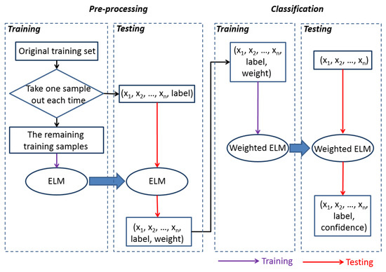
Figure 1.
The flowchart of the automatic solar irradiance classification system (SICS).
The entire SICS consists of two phases, namely, the pre-processing phase and the classification phase. Each of these two phases contains a training process and a testing process. The goal of the pre-processing phase is to pre-assign a weight to each training sample indicating roughly the confidence level of that sample according to the traditional ELM system. Each training data sample is assigned with a label ‘−1’ or ‘1’ with a weight that is automatically calculated by the traditional ELM, taking the remaining training samples as the training dataset. In the classification phase, the weighted ELM (WELM) is employed [28]. The WELM algorithm refines the confidence levels with the classification probabilities calculated by the WELM. All classification probabilities are normalized to obtain the final confidence level for each testing sample.
2.4. A Simulation Model for Customized Maximum Power Point Tracker (MPPT) Design
The customized MPPT design is established according to the following steps. First, the solar irradiance data is divided into training and testing datasets. The training dataset samples include days that can be easily labeled as ‘1’ and ‘−1’. The testing dataset contains samples which are ambiguous for manual identification. Second, both training and testing dataset are processed by a pre-training phase. The WELM models are trained using the training dataset. Third, MATLAB/Simulink is used to select the optimal step size of the coast, desert and coast-desert types. Fourth, the 0 type days are double checked to increase the classification accuracy. The days are ranked by associated confidence level. Three different MPPT step size are applied to run the simulation. A threshold can be obtained to further separate 1 and −1 from 0 type.
To make our simulation repeatable, we deliberately chosen a simulation example from Simulink library, titled ‘Average Model of a 100-kW Grid-Connected PV Array’ as the template. Matlab R2018a is used for this simulation. A detailed description of this file is provided in the Matlab ‘Help’ document. In this simulation model, a two-stage grid-connected PV inverter is simulated. It includes four parts, PV array, dc/dc boost converter, dc/ac voltage source converter (VSC) and utility grid (connected via a transformer). The simulation setup is shown in Figure 2. The MPPT step size can be set up in the box at the left up corner named ‘MPPT parameters’. The initial duty cycle (D) for the boost converter is 0.5. The upper limit, lower limit and the incremental size are 0.8, 0.2 and 0.001, respectively. The global horizontal irradiance (GHI) data has been used as input to the simulation model and it can be set up in the box at the left bottom corner named ‘Irradiance’. A dataset with 9 hours and 60 second sampling rate is used, which means that there are 540 data points for one day.
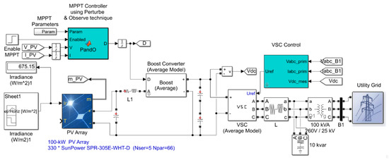
Figure 2.
MATLAB/Simulink circuit diagram for maximum power point tracker (MPPT) step size selection simulation.
3. Results and Discussion
3.1. Classification Results
The two models, ELM and SVM, have high accuracy in identifying the weather type. For the ELM model, the testing data has 365 samples. It includes 178 samples of 1, 134 samples of 0 and 53 samples of −1. The ELM model’s output results have 20 errors that include 8 samples of 1, 11 samples of 0 and 1 sample of −1. The accuracy rates of 1, 0 and −1 in the ELM model are 95.51%, 91.79% and 98.11%, respectively. The overall accuracy is 94.52%. After analyzing the misclassified data, all error samples of 1 and −1 have been wrongly identified as 0. No mistake has been found for misidentification of 1 as −1 or −1 as 1.
For the SVM model, the testing dataset has 365 samples, including 174 samples of 1, 135 samples of 0 and 56 samples of −1. The SVM model’s output results have 28 errors that consist of 6 samples of 1, 21 samples of 0 and 1 sample of −1. The accuracy rates of 1, 0 and −1 for the SVM model are 95.56%, 84.44% and 98.21%. The overall accuracy is 92.33%. After analyzing the misclassified samples, all the error samples of 1 and −1 have been wrongly identified as 0. No mistake has been found for misidentification between 1 and −1.
The comparison of the results from the two models in total and specific weather type are shown in Table 1 and Table 2.

Table 1.
Detail of testing data.
Table 2.
Detail of the testing data with the specific weather type.
To conclude, the ELM model has better performance in identifying 0; and the SVM model has better performance in identifying 1. The ELM model has better overall accuracy than the SVM model.
There is a significant difference in the daily irradiance waveform between the coast type and desert type. The coast-desert type means that the fluctuation and smoothness of the solar irradiance waveform both exist in one day. From Table 2, we can find that there is a relatively large number of days classified as 0. For different classification, the optimal step size can be different. The optimal step size of the coast-desert type is between the one for coast type and desert type. The optimal step size is decided by the degree of fluctuation.
It is a challenge to precisely classify these days into one of these three categories only from the plotted irradiance waveform. We find the confidence level of the WELM results correspond highly to the degree of the fluctuation. Higher confidence level associated with higher level of fluctuation. Figure 3 shows the variation of the GHI with the increments of the confidence levels. The confidence levels of specific dates are shown in Table 3 and Table 4.
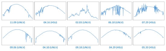
Figure 3.
Variation of the global horizontal irradiance (GHI) with the increments of the confidence levels.
Table 3.
Weighted ELM (WELM) confidence level of some specific dates for estimating 1.
Table 4.
WELM confidence level of some specific dates for estimating −1.
The confidence levels for a whole year have been shown in Figure 4. The confidence level has been normalized. The black/white colors represent the days with large/small irradiance variation. The grey color is the days with mixed situation. It can be seen from the map that the days with similar irradiance situation are clustered together. There is a possibility to further optimize the MPPT for each cluster.
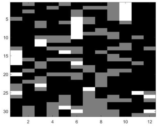
Figure 4.
Humboldt State University’s (HSU) grey-scale map with three colors for a whole year data. The horizontal axis indicates the number of months and the vertical axis indicates the number of days in a month. The grey-scale levels show different confidence levels of the classification results. The black/white colors represent the days with large/small irradiance variation. The grey color is the days with mixed situation.
3.2. MPPT Simulation Results
The optimal step sizes for the three types of irradiance conditions are obtained by using MATLAB/Simulink to simulate the MPPT performance under different conditions. One day which has the most representative features for each type of weather has been selected; six different step sizes (0.03, 0.02, 0.015, 0.01, 0.002 and 0.0002) are chosen to evaluate the MPPT performance. After evaluating the simulation results for all the cases, the optimal step size is selected by comparing the yield energy. The simulation results are shown in Table 5.
Table 5.
Simulation results for optimal MPPT step size sweeping.
A threshold is determined using the WELM model’s output results to classify the three types. All −1 type samples’ confidence level are converted to negative numbers. The threshold is set by using the simulation model to simulate the energy produced by using the three type’s optimal step size (0.002, 0.01 and 0.02). The two boundary points of two types are set as thresholds. Table 6 shows the energy produced with different step sizes. For days classified as 0 type by the WELM, if its confidence level is smaller than −0.01 or larger than 0.81, it will be corrected as −1 or 1 respectively.
Table 6.
The energy produced with different step sizes.
To verify the effectiveness of the selected threshold, the trained WELM model is again tested using the testing data from HSU and UNLV. The confidence level and threshold are used to classify the new dataset. As shown in Table 7, the MATALB model is used to verity if the model using optimal step size can produce maximum energy. All these three days have been classified as 0 by the WELM model, and are very hard to classify by humans. However, the first and third data confidence levels fall out the threshold boundary. They should be corrected as −1 and 1 respectively. The simulation results approved the effectiveness of this method.
Table 7.
Simulation results of new testing data.
4. Conclusions
A customized MPPT design was proposed to determine the optimal step sizes according to three different weather types. The weather-type labeling was automatically provided by a supervised learning classification system. Two classical machine learning technologies were employed and compared, including SVM and ELM. The classification probability from SVM or ELM is deployed as the confidence level and is designed as a fuzzy-weighted classification system to further improve the MPPT design. The simulation result shows the proposed hybrid MPPT outperformed the traditional fixed-step size P&O methods. Because of the localized design method, the proposed method can achieve high MPPT efficiency by using a low-cost simple micro-controller. This solution will become more attractive when the MPPT controller is further adopted at a sub-module level, which means many more MPPT controllers are needed.
Author Contributions
Conceptualization, Y.D. and K.Y.; Methodology, Y.D.; Software, Y.D.; Validation, Y.D., K.Y. and Z.R.; Formal Analysis, K.Y.; Investigation, W.X.; Resources, Y.D.; Data Curation, Z.R.; Writing-Original Draft Preparation, K.Y.; Writing-Review & Editing, Y.D.; Visualization, Y.D.; Supervision, W.X.; Project Administration, K.Y.; Funding Acquisition, K.Y. and Y.D.
Funding
This research is supported by the National Natural Science Foundation of China (61850410531 and 61803315), research development fund of XJTLU (RDF-17-01-28), Key Program Special Fund in XJTLU (KSF-A-11), and Jiangsu Science and Technology Program (SBK2018042034).
Conflicts of Interest
The authors declare that they have no competing interests.
References
- Liu, Y.H.; Huang, S.C.; Huang, J.W.; Liang, W.C. A Particle Swarm Optimization-Based Maximum Power Point Tracking Algorithm for PV Systems Operating Under Partially Shaded Conditions. IEEE Trans. Energy Convers. 2012, 27, 1027–1035. [Google Scholar] [CrossRef]
- Zsiborács, H.; Bai, A.; Popp, J.; Gabnai, Z.; Pályi, B.; Farkas, I.; Baranyai, N.H.; Veszelka, M.; Zentkó, L.; Pintér, G. Change of Real and Simulated Energy Production of Certain Photovoltaic Technologies in Relation to Orientation, Tilt Angle and Dual-Axis Sun-Tracking: A Case Study in Hungary. Sustainability 2018, 10, 1394. [Google Scholar] [CrossRef]
- Zsiborács, H.; Baranyai, N.H.; Vincze, A.; Háber, I.; Pintér, G. Economic and Technical Aspects of Flexible Storage Photovoltaic Systems in Europe. Energies 2018, 11, 1445. [Google Scholar] [CrossRef]
- Salas, V.; Olias, E.; Barrado, A.; Lazaro, A. Review of the maximum power point tracking algorithms for stand-alone photovoltaic systems. Sol. Energy Mater. Sol. Cells 2006, 90, 1555–1578. [Google Scholar] [CrossRef]
- Li, X.; Wen, H.; Jiang, L.; Lim, E.G.; Du, Y.; Zhao, C. Photovoltaic modified β-parameter-based mppt method with fast tracking. J. Power Electron. 2016, 16, 9–17. [Google Scholar] [CrossRef]
- Esram, T.; Chapman, P.L. Comparison of Photovoltaic Array Maximum Power Point Tracking Techniques. IEEE Trans. Energy Convers. 2007, 22, 439–449. [Google Scholar] [CrossRef]
- Mills, A.; Ahlstrom, M.; Brower, M.; Ellis, A.; George, R.; Hoff, T.; Kroposki, B.; Lenox, C.; Miller, N.; Stein, J.; et al. Understanding Variability and Uncertainty of Photovoltaics for Integration with the Electric Power System. Electr. J. 2010. Available online: https://pubarchive.lbl.gov/islandora/object/ir:153901/ (accessed on 30 September 2018).
- Veerapen, S.; Wen, H.; Du, Y. Design of a novel MPPT algorithm based on the two stage searching method for PV systems under partial shading. In Proceedings of the Future Energy Electronics Conference and ECCE Asia (IFEEC 2017-ECCE Asia), Kaohsiung, Taiwan, 3–7 June 2017; pp. 1494–1498. [Google Scholar]
- Zsiborács, H.; Pályi, B.; Pintér, G.; Popp, J.; Balogh, P.; Gabnai, Z.; Pető, K.; Farkas, I.; Baranyai, N.H.; Bai, A. Technical-economic study of cooled crystalline solar modules. Sol. Energy 2016, 140, 227–235. [Google Scholar] [CrossRef]
- Yan, K.; Du, Y.; Ren, Z. MPPT Perturbation Optimization of Photovoltaic Power Systems Based on Solar Irradiance Data Classification. IEEE Trans. Sustain. 2018. [Google Scholar] [CrossRef]
- Du, Y.; Li, X.; Wen, H.; Xiao, W. Perturbation optimization of maximum power point tracking of photovoltaic power systems based on practical solar irradiance data. In Proceedings of the 2015 IEEE 16th Workshop on Control and Modeling for Power Electronics (COMPEL), Vancouver, BC, Canada, 12–15 July 2015. [Google Scholar]
- Yan, K.; Ji, Z.; Lu, H.; Huang, J.; Shen, W.; Xue, Y. Fast and Accurate Classification of Time Series Data Using Extended ELM: Application in Fault Diagnosis of Air Handling Units. IEEE Trans. Syst. Man Cybern. Syst. 2017, 99, 1–8. [Google Scholar] [CrossRef]
- Pashiardis, S.; Kalogirou, S.A.; Pelengaris, A. Statistical analysis for the characterization of solar energy utilization and inter-comparison of solar radiation at two sites in Cyprus. Appl. Energy 2017, 190, 1138–1158. [Google Scholar] [CrossRef]
- Yan, K.; Ji, Z.; Shen, W. Online Fault Detection Methods for Chillers Combining Extended Kalman Filter and Recursive One-class SVM. Neurocomputing 2017, 228, 205–212. [Google Scholar] [CrossRef]
- Femia, N.; Petrone, G.; Spagnuolo, G.; Vitelli, M. A Technique for Improving P&O MPPT Performances of Double-Stage Grid-Connected Photovoltaic Systems. IEEE Trans. Ind. Electron. 2009, 56, 4473–4482. [Google Scholar]
- Xiao, W.; Dunford, W.G.; Palmer, P.R.; Capel, A. Application of Centered Differentiation and Steepest Descent to Maximum Power Point Tracking. IEEE Trans. Ind. Electron. 2007, 54, 2539–2549. [Google Scholar] [CrossRef]
- Shankar, G.; Mukherjee, V. MPP detection of a partially shaded PV array by continuous GA and hybrid PSO. Ain Shams Eng. J. 2015, 6, 471–479. [Google Scholar] [CrossRef]
- Messalti, S.; Harrag, A.; Loukriz, A. A new variable step size neural networks MPPT controller: Review, simulation and hardware implementation. Renew. Sustain. Energy Rev. 2017, 68, 221–233. [Google Scholar] [CrossRef]
- Telbany, M.E.E.; Youssef, A.; Zekry, A.A. Intelligent Techniques for MPPT Control in Photovoltaic Systems: A Comprehensive Review. In Proceedings of the 2014 4th International Conference on Artificial Intelligence with Applications in Engineering and Technology, Kota Kinabalu, Malaysia, 3–5 December 2014. [Google Scholar]
- Ke, Y.; Wen, S.; Mulumba, T.; Afshari, A. ARX model based fault detection and diagnosis for chillers using support vector machines. Energy Build. 2014, 81, 287–295. [Google Scholar]
- Lv, Y.; Liu, J.; Yang, T.; Zeng, D. A novel least squares support vector machine ensemble model for NOx emission prediction of a coal-fired boiler. Energy 2013, 55, 319–329. [Google Scholar] [CrossRef]
- Kaytez, F.; Taplamacioglu, M.C.; Cam, E.; Hardalac, F. Forecasting electricity consumption: A comparison of regression analysis, neural networks and least squares support vector machines. Int. J. Electr. Power Energy Syst. 2015, 67, 431–438. [Google Scholar] [CrossRef]
- Suykens, J.A.K.; De Brabanter, J.; Lukas, L.; Vandewalle, J. Weighted least squares support vector machines: Robustness and sparse approximation. Neurocomputing 2002, 48, 85–105. [Google Scholar] [CrossRef]
- Huang, G.B.; Zhu, Q.Y.; Siew, D.C.K. Extreme learning machine: Theory and applications. Neurocomputing 2006, 70, 489–501. [Google Scholar] [CrossRef]
- Hecht-Nielsen, R. Theory of the backpropagation neural network. In Proceedings of the International 1989 Joint Conference on Neural Networks, Washington, DC, USA, 18–22 June 1989. [Google Scholar] [CrossRef]
- Gardner, M.W.; Dorling, S.R. Artificial neural networks (the multilayer perceptron)—A review of applications in the atmospheric sciences. Atmos. Environ. 1998, 32, 2627–2636. [Google Scholar] [CrossRef]
- Suykens, J.A.K.; Vandewalle, J. Least Squares Support Vector Machine Classifiers. Neural Process. Lett. 1999, 9, 293–300. [Google Scholar] [CrossRef]
- Zong, W.; Huang, G.B.; Chen, Y. Weighted extreme learning machine for imbalance learning. Neurocomputing 2013, 101, 229–242. [Google Scholar] [CrossRef]
- Localized MPPT for PV Systems Using Fuzzy-Weighted ELM. Available online: http://www.keddiyan.com/files/FuzzyWELM.html (accessed on 30 September 2018).
© 2018 by the authors. Licensee MDPI, Basel, Switzerland. This article is an open access article distributed under the terms and conditions of the Creative Commons Attribution (CC BY) license (http://creativecommons.org/licenses/by/4.0/).