Daily Peak Load Forecasting Based on Complete Ensemble Empirical Mode Decomposition with Adaptive Noise and Support Vector Machine Optimized by Modified Grey Wolf Optimization Algorithm

Abstract

Daily peak load forecasting is an important part of power load forecasting. The accuracy of its prediction has great influence on the formulation of power generation plan, power grid dispatching, power grid operation and power supply reliability of power system. Therefore, it is of great significance to construct a suitable model to realize the accurate prediction of the daily peak load. A novel daily peak load forecasting model, CEEMDAN-MGWO-SVM (Complete Ensemble Empirical Mode Decomposition with Adaptive Noise and Support Vector Machine Optimized by Modified Grey Wolf Optimization Algorithm), is proposed in this paper. Firstly, the model uses the complete ensemble empirical mode decomposition with adaptive noise (CEEMDAN) algorithm to decompose the daily peak load sequence into multiple sub sequences. Then, the model of modified grey wolf optimization and support vector machine (MGWO-SVM) is adopted to forecast the sub sequences. Finally, the forecasting sequence is reconstructed and the forecasting result is obtained. Using CEEMDAN can realize noise reduction for non-stationary daily peak load sequence, which makes the daily peak load sequence more regular. The model adopts the grey wolf optimization algorithm improved by introducing the population dynamic evolution operator and the nonlinear convergence factor to enhance the global search ability and avoid falling into the local optimum, which can better optimize the parameters of the SVM algorithm for improving the forecasting accuracy of daily peak load. In this paper, three cases are used to test the forecasting accuracy of the CEEMDAN-MGWO-SVM model. We choose the models EEMD-MGWO-SVM (Ensemble Empirical Mode Decomposition and Support Vector Machine Optimized by Modified Grey Wolf Optimization Algorithm), MGWO-SVM (Support Vector Machine Optimized by Modified Grey Wolf Optimization Algorithm), GWO-SVM (Support Vector Machine Optimized by Grey Wolf Optimization Algorithm), SVM (Support Vector Machine) and BP neural network to compare with the CEEMDAN-MGWO-SVM model and analyze the forecasting results of the same sample data. The experimental results fully demonstrate the reliability and effectiveness of the CEEMDAN-MGWO-SVM model proposed in this paper for daily peak load forecasting, which shows the strong generalization ability and robustness of the model.

1. Introduction

The development of modern society is inseparable from the supply of electricity. The power industry plays a crucial role in promoting social and economic development and improving people’s living standards. With the rapid development of the power industry, the precision of power system for power load forecasting is becoming more and more demanding. Daily peak load forecasting is an important part of power load forecasting. The accuracy of its prediction has great influence on the formulation of power generation plan, power grid dispatching, power grid operation and power supply reliability of power system. Therefore, it is of great significance to construct a suitable model to realize the accurate prediction of the daily peak load.

The core problem of load forecasting is the method and model of prediction. With the rapid development of science and technology, the technology of load forecasting is also being deepened. At present, load forecasting technology has gradually transferred from traditional prediction method to artificial intelligence prediction technology. Traditional load forecasting methods, such as time series method, regression analysis method and grey prediction method [1,2,3], have some shortcomings. The forecasting accuracy of traditional methods for complex load series with larger volatility needs to be improved. However, the artificial intelligence prediction method shows a strong superiority in the face of complex load sequence, and has achieved good prediction effect [4]. The artificial neural network (ANN) algorithm, originating in the 1940s, is an artificial intelligence technology, which simulates the biological process of human brain [5]. The BP (Back Propagation) algorithm, also known as the error back propagation algorithm, is a supervised learning algorithm in artificial neural networks, which is often used for load forecasting [6,7]. Wang et al. [8] put forward a new back-propagation neural network algorithm to apply it in the semi-distributed model. The improved hydrological model could update the flow forecasting error without losing the leading time. However, BP neural network algorithm has some disadvantages, such as slow convergence speed, long training time, easy to fall into local optimal solution and so on [9,10]. Support vector machine (SVM) is a small sample machine learning method based on the theory of VC (Vapnik-Chervonenkis) dimension of statistical learning theory and the principle of minimum structure risk. It seeks the best compromise between the complexity of the model and the learning ability based on the limited sample information to achieve the best promotion [11,12,13]. Wei et al. [14] used the seeker optimization algorithm to get the optimal parameters selection of SVM. Then the short-term load prediction of the next 24 h in one region was achieved by the SVM model based on the historical load data as input. Support vector machine algorithm has strong generalization ability, fast convergence speed, and can avoid falling into local optimal solution [15,16]. At present, many optimization algorithms, such as particle swarm optimization (PSO), simulated annealing (SA) and genetic algorithm (GA), are proposed for the optimization of SVM parameters. Huang and Dun [17] put forward a novel PSO–SVM model that hybridized the particle swarm optimization and support vector machines to improve the classification accuracy with a small and appropriate feature subset. Liu and Huang [18] used simulated annealing algorithm (SA) to optimize the parameters of SVM and proposed a model based on simulated annealing algorithm and support vector machine to forecast the power load that has proven to be of good prediction effect. Wang et al. [19] put forward a forecasting model based on environmental factors and support vector machine optimized by genetic algorithm to predict the short-term PV power using the gray correlation coefficient algorithm to find out a similar day of the predicted day. In this paper, the grey wolf optimization algorithm is used to optimize the parameters of support vector machine. GWO (Grey Wolf Optimization) algorithm is a new meta heuristic optimization algorithm proposed by Mirjalili et al. in 2014. It is a new swarm intelligence optimization algorithm, has superior performance in finding optimal solutions, and is simple and efficient [20,21,22]. Xu and Ding [23] put forward the model of Grey wolf optimization algorithm which is improved by extremal optimization and support vector machine for cloud computing resource load short-term forecasting and tested the performance of EGWO-SVM by simulation experiments. The experimental results showed that the proposed model could precisely characterize the complicated trends of cloud computing resource short-term load and efficiently promote the short-term resource load prediction accuracy.

The daily peak load forecasting is easily disturbed by external factors, and the load sequence contains some noise and strong volatility, which brings great difficulties to the prediction work. Wavelet decomposition and empirical mode decomposition are two effective time frequency analysis methods to deal with non-stationary signals. The wavelet decomposition gradually refines the signal through the telescopic translation operation, and finally realizes the time subdivision at high frequency and the frequency subdivision at low frequency [24,25,26]. Seo et al. [27] proposed two hybrid models for daily water level forecasting. They were wavelet-based artificial neural network and wavelet-based adaptive neuro-fuzzy inference system. It was proven that the combination of wavelet decomposition and artificial intelligence models can be a useful tool for accurate forecasting daily water level through empirical analysis. The essence of empirical mode decomposition is to smooth the signal, and decompose the complex signal into Intrinsic Mode Function (IMF) [28,29,30]. Premanode and Toumazou [31] put forward the differential Empirical Mode Decomposition (EMD) for improving prediction of exchange rates under support vector regression (SVR), which has the capability of smoothing and reducing the noise. Compared with the traditional forecasting methods, the hybrid EMD-SVM forecasting method could effectively improve the forecasting accuracy and track the change of wind power. Compared with the wavelet decomposition, empirical mode decomposition is not affected by the selection of wavelet base and the number of decomposition layers, but based on the adaptability of data itself, and the noise reduction performance of load sequence is better. Based on the traditional EMD, Ensemble Empirical Mode Decomposition (EEMD) adopted Gauss white noise to reduce the generation of modal aliasing in a certain range [32,33]. Jiang et al. [34] proposed a hybrid approach based on the ensemble empirical mode decomposition and grey support vector machine for short-term high-speed rail passenger flow forecasting. However, due to the addition of white noise sequences, the accuracy of the EEMD algorithm reconstruction sequence will be affected. Therefore, based on previous studies of EEMD, Colominas proposed the Complete Ensemble Empirical Mode Decomposition with Adaptive Noise (CEEMDAN). The CEEMDAN method adds adaptive white noise smooth pulse interference in each decomposition to make the decomposition of the signal data more complete [35,36,37]. Jun and Qing [38] developed an effective combined model based on complete ensemble empirical mode decomposition with adaptive noise, permutation entropy and echo state network with leaky integrator neurons for medium-term power load forecasting. Therefore, in this paper, we choose the CEEMDAN method to do the noise reduction for the daily peak load sequence.

A novel daily peak load forecasting model of CEEMDAN-MGWO-SVM is proposed in this paper. Firstly, the model uses the complete ensemble empirical mode decomposition with adaptive noise (CEEMDAN) algorithm to decompose the daily peak load sequence into multiple sub sequences. Then, the model of modified grey wolf optimization and support vector machine (MGWO-SVM) is adopted to forecast the sub sequences. Finally, the forecasting sequence is reconstructed and the forecasting result is obtained. The model provides a new idea for daily peak load forecasting. The main contents and structure of this paper are as follows: Section 2 introduces the algorithm of complete ensemble empirical mode decomposition with adaptive noise (CEEMDAN), which is used to reduce the noise of non-stationary daily peak load sequence. Section 3 introduces the MGWO-SVM model, which is the core algorithm for daily peak load forecasting in this paper. The model adopts the grey wolf optimization algorithm improved by introducing the population dynamic evolution operator and the nonlinear convergence factor to enhance the global search ability and avoid falling into the local optimum, which can better optimize the parameters of the SVM algorithm for improving the forecasting accuracy of daily peak load. Section 4 introduces the forecasting process of the CEEMDAN-MGWO-SVM model. Section 5 carries out an empirical analysis. Three cases are taken to test the forecasting accuracy of the CEEMDAN-MGWO-SVM model. We choose the models of EEMD-MGWO-SVM, MGWO-SVM, GWO-SVM, SVM and BP neural network to compare with the CEEMDAN-MGWO-SVM model and analyze the forecasting results of the same sample data, which proves the superiority of the CEEMDAN-MGWO-SVM model. Section 6 summarizes the full text.

2. Complete Ensemble Empirical Mode Decomposition with Adaptive Noise

2.1. EMD

The Empirical Mode Decomposition (EMD), which is the core of Hilbert–Huang Transform (HHT), is a technique to stabilize signals and decompose the complex signal into a finite number of Intrinsic Mode Functions (IMFs) containing local characteristic signals at different time scales [28,29,30]. The EMD should meet the following two requirements:

(1)

either the number of extrema and the number of zero crossings are equal or differ at most by one; and

(2)

the mean value of the upper envelope and the lower envelope is zero.

For a given signal $X\left(t\right)$, the result after decomposition is given by

$$X(t)={\displaystyle \sum _{i=1}^{n}im{f}_i(t)}+r_n(t)$$

(1)

where $im{f}_i(t)$ is the component of IMF containing local characteristic signals at different time scales, and $r_n(t)$ is the residual signal.

Detailed steps of the EMD are as follows:

(1)

Determine all the local extremum points of $X\left(t\right)$, and fit the upper envelope and the lower envelope respectively with the cubic spline function.

(2)

Compute the mean value $f_m(t)$ of upper and lower envelopes.

(3)

Compute the difference of $X(t)$ and $f_m(t)$, where $E(t)=X(t)-f_m(t)$.

(4)

Set $E\left(t\right)$ as the original sequence, repeat Step (1) to Step (3), and then obtain the first IMF component $im{f}_1(t)$ when envelope mean tends to be zero.

(5)

Define $X_1(t)=X(t)-im{f}_1(t)$ and set $X_1(t)$ as the original sequence; repeat above steps until the residual signal $r_n(t)$ becomes a constant function or monotonic function; and then end the decomposition.

2.2. EEMD

The Ensemble Empirical Mode Decomposition (EEMD) adds the Gaussian white noise into traditional EMD to solve the problem of mode mixing [32,33]. Detailed steps are as follows:

(1)

Add the Gaussian white noise $n_j(t)$ into given original signal $X\left(t\right)$ to obtain the signal $X_I(t)$:

$$X_I(t)=X(t)+n_j(t)$$

(2)

(2)

Carry out the EDM decomposition on signal $X_I(t)$ to get the IMF component $M_{ij}(t)$ which is the $j$th IMF component after EMD decomposition when adding the Gaussian white noise at the $i$th time.

(3)

Repeat Step (1) and Step (2) for $N$ times, and add different Gaussian white noise each time.

(4)

Set the mean value of IMF components of N-time decomposition as the final IMF:

$$M_j\left(t\right)=\frac{1}{N}{\displaystyle \sum _{i=1}^N{M}_{ij}}(i=1,2,\cdots ,Nj=1,2,\cdots ,M)$$

(3)

2.3. CEEMDAN

Although EEMD can reduce mode mixing to a certain degree, due to the newly added white noise sequence, the error cannot be completely eliminated after a finite number of averaging computation, affecting the accuracy of the reconstruction sequence. Therefore, based on previous studies of EEMD, Colominas proposed the Complete Ensemble Empirical Mode Decomposition with Adaptive Noise (CEEMDAN), which adds adaptive white noise smoothing pulse interference in decomposition, and utilizes the characteristic of mean Gaussian white noises whose mean equals to zero to make the decomposition of signal data more complete, thus to effectively eliminate mode mixing [35,36,37].

Detailed steps of CEEMDAN are as follows:

(1)

Consistent with the EEMD, in N-times computation of CEEMDAN, decompose the signal $X(t)+p_i{n}_j(t)$, where the parameter $p_i$ controls the signal-to-noise ratio of the additional noise to the original signal. The first IMF component is:

$$\overline{IM{F}_1(t)}=\frac{1}{N}{\displaystyle \sum _{j=1}^{N}IM{F}_1^j(t)}$$

(4)

The residual signal is:

$$r_1(t)=X(t)-\overline{IM{F}_1(t)}$$

(5)

(2)

Define $emd\left(t\right)$ as the $k$th IMF component by EMD, and then decompose the sequence $r_1(t)+p_{1}em{d}_1(n_j(t))$ to get the second IMF component as

$$\overline{IM{F}_2(t)}=\frac{1}{N}{\displaystyle \sum _{j=1}^{N}em{d}_1(}{r}_1(t)+p_{1}em{d}_1(n_j(t)))$$

(6)

The residual signal is:

$$r_2(t)=r_1(t)-\overline{IM{F}_2(t)}$$

(7)

(3)

Similar to what has been carried out above, the $k$th residual signal can be expressed by

$$r_k(t)=r_{k-1}(t)-\overline{IM{F}_k(t)}$$

(8)

The $k+1$th IMF component can be expressed by:

$$\overline{IM{F}_{k+1}(t)}=\frac{1}{N}{\displaystyle \sum _{j=1}^{N}em{d}_1(}{r}_k(t)+p_{k}em{d}_k(n_j(t)))$$

(9)

(4)

Repeat above steps until the residual signal meets the requirement of ending criterion. Supposing that there are $L$ IMF components, the original sequence can be expressed by:

$$X(t)={\displaystyle \sum _{i=1}^L\overline{IM{F}_i(t)}+r(t)}$$

(10)

where $r(t)$ is the final residual signal.

3. Support Vector Machine Optimized by Modified Grey Wolf Optimization Algorithm

3.1. SVM

Support Vector Machine (SVM) is a kind of machine learning method based on the principle of VC dimension of statistical learning theory and the principle of structural risk minimization. Based on limited sample information, SVM seeks the best compromise between model complexity and learning ability, and obtains the best promotion ability [11,12,13].

When SVM is used for forecasting, the input samples are mapped into high dimensional feature space $H$ through loss function $\phi (x_i)$, and linear regression is carried out. The regression function of SVM in high dimensional feature space is:

$$f(x_i)={\omega }^T\phi (x_i)+b$$

(11)

where $\omega$ is the weight vector of high dimensional feature space, $\omega \in R^k$; and $b$ is the bias constant, $b\in R$.

According to the principle of structural risk minimization, Equation (11) can be converted into:

$$\begin{array}{l}\min J=\frac{1}{2}{\Vert \omega \Vert }^2+c{\displaystyle \sum _{i=1}^n({\xi }_i+{\xi }_i{}^{*})}\\ s.t.\{\begin{array}{c}{y}_i-{\omega }^T\phi (x_i)-b\le \epsilon +{\xi }_i\\ {\omega }^T\phi (x_i)+b-y_i\le \epsilon +{\xi }_i\\ {\xi }_i,{\xi }_i{}^{*}\ge 0(i=1,2,\cdots ,n)\end{array}\end{array}$$

(12)

where ${\Vert \omega \Vert }^2$ controls the complexity of this model, $c$ is the regularization parameter, $\epsilon$ is the insensitive coefficient; ${\xi }_i$ and ${\xi }_i{}^{*}$ are relaxation factors.

Introducing the Lagrange multipliers into the model to convert the problem into convex quadratic optimization problem:

$$\begin{array}{cc}\hfill L(\omega ,{\xi }_i,{\xi }_i{}^{*},\alpha ,{\alpha }^{*},c,\beta ,{\beta }^{*})=& \frac{1}{2}{\Vert \omega \Vert }^2+c{\displaystyle \sum _{i=1}^n({\xi }_i+{\xi }_i{}^{*})}\hfill \\ & -{\displaystyle \sum _{i=1}^n{\alpha }_i\left[{\omega }^T\phi (x_i)+b-y_i+\epsilon +{\xi }_i\right]}\hfill \\ & -{\displaystyle \sum _{i=1}^n{\alpha }_i{}^{*}\left[y_i-{\omega }^T\phi (x_i)-b+\epsilon +{\xi }_i{}^{*}\right]}\hfill \\ & -{\displaystyle \sum _{i=1}^n({\beta }_i{\xi }_i+{\beta }_i{}^{*}{\xi }_i{}^{*})}\hfill \end{array}$$

(13)

where ${\alpha }_i,{\alpha }_i{}^{*},{\beta }_i,{\beta }_i{}^{*}$ are Lagrange multipliers, and they meet the requirement of ${\alpha }_i>0, {\alpha }_i{}^{*}>0, {\beta }_i>0, {\beta }_i{}^{*}>0 (i=1,2,\cdots ,n)$.

To speed up computation, Equation (13) is converted into its dual form:

$$\begin{array}{c}\max W(\alpha ,{\alpha }^{*})=-\frac{1}{2}{\displaystyle \sum _{i,j=1}^n(a_i-a_i{}^{*})}(a_j-a_j{}^{*})\phi {(x_i)}^T\phi (x_j)\hfill \\ +{\displaystyle \sum _{i=1}^n(a_i-a_i{}^{*})}{y}_i-{\displaystyle \sum _{i=1}^n(a_i-a_i{}^{*})}\epsilon \hfill \\ s.t.\{\begin{array}{c}{\displaystyle \sum _{i=1}^n(a_i-a_i{}^{*})}=0\\ 0\le a_i,a_i{}^{*}\le c\end{array}\hfill & \end{array}$$

(14)

The kernel function $K(x_i,x_j)$ is taken to replace of inner product of vectors $\phi {(x_i)}^T\phi (x_j)$ in high-dimensional space to avoid dimensionality disaster, and the regression function of SVM is:

$$f(x)={\displaystyle \sum _{i=1}^n({\alpha }_i-{\alpha }_i{}^{*})K(x_i,x_j)}+b$$

(15)

In this paper, the radial basis function is used as the kernel function which is given by:

$$K(x_i,x_j)=\exp \left(\frac{-{\Vert x_i-x_j\Vert }^2}{2{\sigma }^2}\right)$$

(16)

where $\sigma$ is the width of the radial basis function.

3.2. MGWO

3.2.1. GWO

The Grey Wolf Optimization Algorithm (GWO) is a biologically inspired optimization algorithm by simulating the social hierarchy and hunting nature of grey wolf family [20,21]. The grey wolves are gregarious animals, and there are usually a dozen wolves in each pack, which build a strict grey wolf pyramid hierarchy [22].

The alpha ($\alpha$) wolves, who are at the top of the pyramid with the highest authority, are the leader of other wolves. The $\alpha$ wolves are mainly responsible for predation and decision-making, and other wolves must obey theirs command.

The beta ($\beta$) wolves, who are at the second layer of the pyramid with the status second only to the $\alpha$ wolves, are mainly responsible for assisting the $\alpha$ wolves for decision-making. $\beta$ wolves have control over other individuals in the pack and can feed the information of other wolves back to the $\alpha$ wolves.

The delta ($\delta$) wolves, who are at the third layer of the pyramid, are mainly responsible for decision implementation of $\alpha$ wolves and $\beta$ wolves. The status of $\delta$ wolves is higher than that of $\omega$ wolves.

The omega ($\omega$) wolves, who are at the bottom of the pyramid, are mainly responsible for help prey.

In the GWO, the $\alpha$, $\beta$ and $\delta$ wolves are mainly responsible for attacking prey, and $\omega$ wolves are responsible for tracking and encircling until finally successfully capturing the prey.

For mathematical modeling of GWO algorithm which simulates hunting behavior of grey wolves, we need first generate a group of wolves randomly in the search space, then use $\alpha ,\beta$ and $\delta$ wolves to estimate the position of the prey. As for other wolves, they are ordered to calculate the distance between themselves and the $\alpha$, $\beta$ and $\delta$ wolves, then get close to the prey and encircle it, finally capture the prey successfully. Detailed steps are shown in Figure 1.

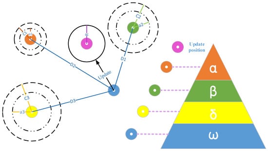
Figure 1. The diagram of GWO (Grey Wolf Optimization) algorithm.

The modeling steps of GWO are as follows: supposing that there are $M$ wolves in a pack and the searching space has $k$ dimensions, the position of grey wolf $i$ can be expressed as $x_i=(x_{i1},x_{i2},\cdots ,x_{ik})$, the behavior of grey wolves encircling the prey can be mathematically expressed using the following equations:

$$d=\left|c\cdot x_p(t)-x(t)\right|$$

(17)

$$x(t+1)=x_p(t)-b\times d$$

(18)

where $t$ is the current iteration, $x(t)$ represents the position of wolves at the $t$th iteration, $x_p(t)$ is the position of the prey. The vector $b$ and $d$ can be obtained by Equations (19) and (20).

$$b=2a{r}_1-a$$

(19)

$$c=2r_2$$

(20)

where $r_1$ and $r_2$ are random vectors ranging from 0 to 1. With the time of iteration increasing, $a$ decreases from 2 to 0.

Assuming that $\alpha$, $\beta$ and $\delta$ wolves are closest to the prey, and we can rely on the position of these three kinds of wolves to estimate the prey’s position, the way to update the position of other wolves is as shown in Equations (21)–(27).

$$d_{\alpha }=\left|c_1\cdot x_{\alpha }-x\right|$$

(21)

$$d_{\beta }=\left|c_2\cdot x_{\beta }-x\right|$$

(22)

$$d_{\delta }=\left|c_3\cdot x_{\delta }-x\right|$$

(23)

$$x_1=x_{\alpha }-b_1\times d_{\alpha }$$

(24)

$$x_2=x_{\beta }-b_2\times d_{\beta }$$

(25)

$$x_3=x_{\delta }-b_3\times d_{\delta }$$

(26)

$$x(t+1)=\frac{x_1+x_2+x_3}{3}$$

(27)

3.2.2. MGWO

For complex optimization problems, the GWO is apt to fall into the local optimal solution. To solve this problem, in this paper, we improve the GWO algorithm by introducing the population dynamic evolution operator and nonlinear convergence factor to effectively avoid falling into the local optimum.

By introducing population dynamic evolution operator, the search range of wolves in GWO algorithm can be expanded to the entire solution space during each iteration of algorithm to increase the probability of obtaining the global optimal solution. Specific steps are as follows:

In the GWO, the wolves update their positions according to the position of $\alpha$ wolves, $\beta$ wolves and $\delta$ wolves. We modify the equations as:

$$x_{\alpha }=x_1\pm (ub-lb\cdot r+lb)$$

(28)

$$x_{\beta }=x_2\pm (ub-lb\cdot r+lb)$$

(29)

$$x_{\delta }=x_3\pm (ub-lb\cdot r+lb)$$

(30)

where $ub$ and $lb$ are the upper and lower bounds of search space, respectively; and $r$ is a random number ranging from 0 to 1.

The updated potential optimal solution vector is:

$$x(t+1)=\frac{x_{\alpha }+x_{\beta }+x_{\delta }}{3}$$

(31)

In GWO, though the convergence factor linearly decreasing from 2 to 0 over the course of iteration, the algorithm cannot be changed linearly in the process of convergence, making the convergence factor $a$ fails to fully reflect the actual optimization search process. Therefore, in this paper, we introduce nonlinear convergence factor to improve the GWO algorithm, as shown in Equation (32):

$$a=2-(e^{\frac{t}{t_{\max }}}-1)\cdot \frac{2}{(e-1)}$$

(32)

where $a$ is the convergence factor. $e$ is the base of natural logarithm, which approximates 2.718. $t$ is the current iteration. $t_{\max }$ is the maximum of iterations.

The convergence trend of $a$ with the increase of iterations is shown in Figure 2.

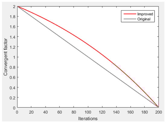
Figure 2. The convergence trend of $a$.

As can be seen in Figure 2, the improved convergence factor $a$ decreases nonlinearly with the increase of iterations. During that process, it decreases slowly in the initial period to facilitate global search, but decreases rapidly in the later period to enhance the local optimization.

3.3. MGWO-SVM

The values of regularization parameter $c$ and radial basis function parameter $g$ have a direct impact on the accuracy of the forecast model of SVM with RBF kernel. In this paper, the MGWO is used to optimize the two parameters of SVM. Based on GWO, the global search ability is improved by introducing the population dynamic evolution operator and nonlinear convergence factor to avoid falling into the local optimum, so as to improve the forecasting accuracy of SVM. Concrete steps of MGWO-SVM are as follows:

Step 1:

Set the ranges of parameters related to the MGWO, regularization parameter $c$ and radial basis function parameter $g$ in SVM.

Step 2:

Randomly initialize the wolf population, and make the position vector of each wolf consist of $c$ and $g$.

Step 3:

Use the initialized SVM to learn the training set and calculate the fitness value of each grey wolf individual.

Step 4:

StepClassify the grey wolves according to the fitness value, and determine the positions of $\alpha$ wolves, $\beta$ wolves, $\delta$ wolves and $\omega$ wolves.

Step 5:

Update positions of the wolves to generate a new population, calculate the corresponding fitness values, and compare them with that of the last iteration, so as to retain the preference.

Step 6:

Determine whether it reaches the maximum iteration, if reached, end the training and output the optimized $c$ and $g$. Otherwise, jump to Step 4 to continue the parameter optimization.

Step 7:

Use the optimized parameters to establish the SVM forecast model and carry out forecast for the test set.

4. The Forecast Model Based on CEEMDAN-MGWO-SVM

The forecasting accuracy of daily peak load is influenced by many factors. To accurately forecast the daily peak load, in this paper, by taking meteorological factors and date types into account, we propose a forecasting model based on CEEMDAN-MGWO-SVM for daily peak load forecasting. Steps for this model are as follows:

(1) Data acquisition and preprocessing

We collect sample data including historical daily peak load, daily maximum temperature, daily minimum temperature, daily average temperature, daily average relative humidity, maximum daily wind speed, date type and other data. Then, data preprocessing is to be carried out, that is, the meteorological data are normalized, and we mark holidays and working days as 1 and 0, respectively.

(2) Sequence de-noising based on CEEMDAN

To obtain multiple IMF components, the CEEMDAN is to be performed on the original daily peak load sequence.

(3) Daily peak load forecast based on MGWO-SVM

Based on considering the meteorological factors and date types, the IMF components derived from CEEMDAN are used to carry out the forecast by MGWO-SVM model, and the forecasting results are reconstructed to obtain the final daily peak load forecast results.

The flow chart of CEEMDAN-MGWO-SVM is shown in Figure 3.

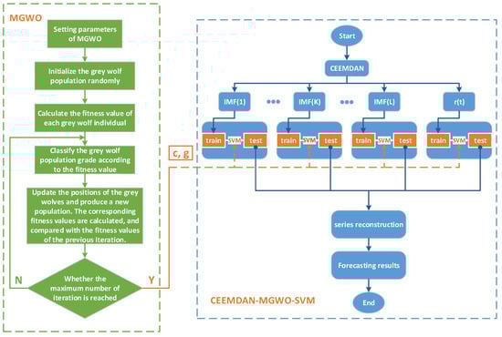
Figure 3. The flow chart of CEEMDAN-MGWO-SVM.

5. Empirical Analysis

5.1. Case 1

5.1.1. Sample Selection

In this paper, the daily peak load of S power grid of 92 days from March to May 2017 is selected as the research object. The daily peak load, daily maximum temperature, daily minimum temperature, daily average temperature, daily average relative humidity, maximum daily wind speed, date type and other data are collected. (The source of the data is State grid Jibei electric power Co., LTD. in Hebei Province, China)

The collected data are shown in Figure 4.

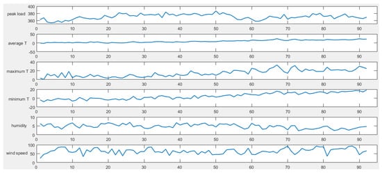
Figure 4. The collected data.

Owing to too many influencing factors, we use the index of Mean Impact Value (MIV) to sift the influence factors for model input. Mean impact value (MIV) is one of the commonly used indexes to evaluate the influence of the independent variable on the dependent variable. The symbol represents the direction of the correlation, and the absolute value represents the relative importance of the influence. Through calculation, the rank of the absolute value of the mean impact value of each influence factor can be obtained, which is shown in Table 1.

Table 1. The rank of the absolute value of the mean impact value of each influence factor.

Influence Factors	$\mathbf{M}\mathbf{I}\mathbf{V}$	$\left|\mathbf{M}\mathbf{I}\mathbf{V}\right|$	Rank
the average daily peak load of one week before the forecasting day	16.19‰	16.19‰	1
daily average relative humidity	−9.17‰	9.17‰	2
the daily peak load of first day before the forecasting day	−8.95‰	8.95‰	3
the daily peak load of second day before the forecasting day	6.88‰	6.88‰	4
date type	6.03‰	6.03‰	5
daily average temperature	−5.84‰	5.84‰	6
the daily maximum temperature	−2.58‰	2.58‰	7
daily minimum temperature	1.38‰	1.38‰	8
maximum daily wind speed	−0.53‰	0.53‰	9
the daily peak load of third day before the forecasting day	−0.04‰	0.04‰	10

According to Table 1, we select the six influence factors that the absolute value of MIV is more than 5‰ as the model input. They are the average daily peak load of one week before the forecasting day, daily average relative humidity, the daily peak load of first day before the forecasting day, the daily peak load of second day before the forecasting day, date type and daily average temperature. The model output is the daily peak load of the forecasting day. We use the data from March to April as the training set sample, and the data of May as the test set sample.

5.1.2. Daily Peak Load Forecasting Based on CEEMDAN-MGWO-SVM Model

Before entering into the proposed model, we have a unit root test for the original daily peak load sequence. The unit root test result is shown in Table 2.

Table 2. The unit root test result.

		t-Statistic	P
Augmented Dickey-Fuller test statistic		−2.477642	0.3384
Test critical values	1% level	−4.063233
	5% level	−3.460516
	10% level	−3.156439

According to Table 2, p is greater than 0.05, which shows that there is a unit root and the original daily peak load sequence is non-stationary.

Therefore, the Complete Ensemble Empirical Mode Decomposition with Adaptive Noise is applied to the original daily peak load sequence. The daily peak load of S power grid from March to May 2017 is used as the signal sequence to input the CEEMDAN model, and six IMFs and one residual signal are obtained. The decomposition result is shown in Figure 5.

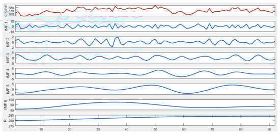
Figure 5. The IMFs (intrinsic mode functions) of CEEMDAN.

The MGWO-SVM model is used to forecast the IMFs and the residual signal, respectively. The parameters of model are set as follows: the number of grey wolf population is 20, the search range of regularization parameter is [0.1, 200], and the search range of RBF kernel parameters is [0.01, 20], and the maximum iteration number is 200. The forecasting results are shown in Figure 6.

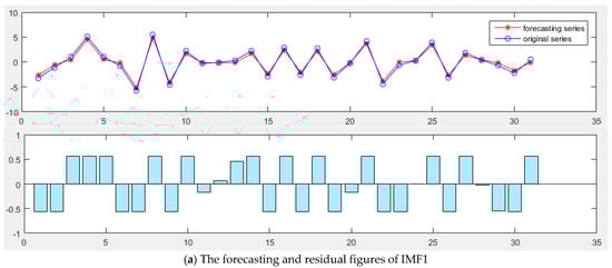
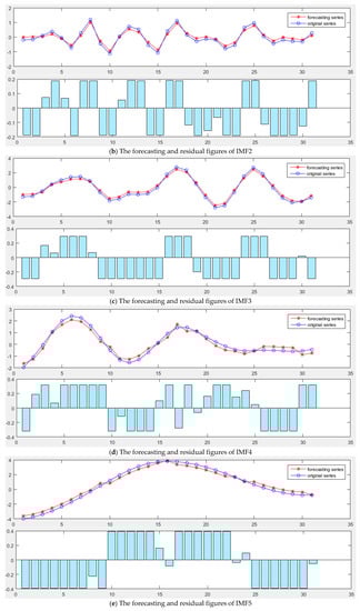
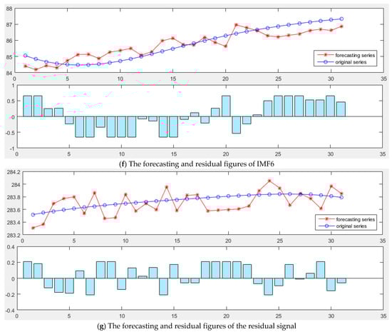
Figure 6. The forecasting results of IMFs: (a) IMF1; (b) IMF2; (c) IMF3; (d) IMF4; (e) IMF5; (f) IMF6; and (g) Residual.

The forecasting results of the IMF components and the residual signal are reconstructed, and the daily peak load forecasting result of the S power grid in May 2017 is shown in Figure 7.

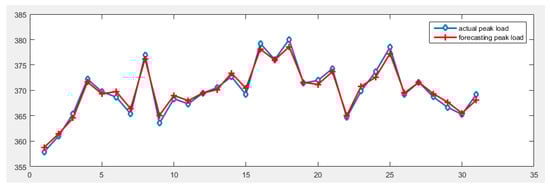
Figure 7. Figure of the final forecasting result (Unit: 10 MW).

As shown in Figure 7, we can see that using the CEEMDAN-MGWO-SVM model to forecast the daily peak load of the S power grid in May can achieve good forecasting effect, and the forecasting curve fits the actual curve very well.

5.1.3. Error analysis

To evaluate the forecasting performance of the CEEMDAN-MGWO-SVM model more accurately, the relative error $RE$, the mean absolute percentage error $MAPE$, nonlinear function goodness of fit $R^2$, Akaike Information Criterion $AIC$ and Bayesian information criterion $BIC$ are used in this paper. The calculation equations of the indexes are as shown in Equations (33)–(37).

$$RE=\frac{\left|{\widehat{y}}_i-y_i\right|}{y_i}\times 100\%$$

(33)

$$MAPE=\frac{1}{n}{\displaystyle \sum _{i=1}^n\left|\frac{{\widehat{y}}_i-y_i}{y_i}\right|}\times 100\%$$

(34)

$$R^2=1-\sqrt{\frac{{\displaystyle \sum _{i=1}^n{({\widehat{y}}_i-y_i)}^2}}{{\displaystyle \sum _{i=1}^n{y}_i{}^2}}}$$

(35)

$$AIC=n\ln \left(RSS/n\right)+2(k+1)$$

(36)

$$BIC=n\ln \left(RSS/n\right)+(k+1)\ln \left(n\right)$$

(37)

where $RSS$ is the residual sum of squares; $n$ is the sample size; and $k$ is the number of independent variables.

Through calculation, we can obtain the $MAPE$, $R^2$, $AIC$ and $BIC$ of the forecasting results of the CEEMDAN-MGWO-SVM model. They are 0.196%, 99.77%, −111.21 and −83.47 respectively. The relative errors of the CEEMDAN-MGWO-SVM model forecasting results are shown in Table 3 and Figure 8.

Table 3. The relative errors of forecasting results.

Date	Actual Value (10 MW)	Forecasting Value (10 MW)	RE (%)
1 May 2017	357.9142	358.8081	0.2498
2 May 2017	361.0432	361.4588	0.1151
3 May 2017	365.4022	364.5513	0.2329
4 May 2017	372.2178	371.6485	0.1530
5 May 2017	369.7462	369.3221	0.1147
6 May 2017	368.6838	369.7757	0.2962
7 May 2017	365.3786	366.3970	0.2787
8 May 2017	376.9988	376.2136	0.2083
9 May 2017	363.5410	365.1021	0.4294
10 May 2017	368.3584	368.9984	0.1737
11 May 2017	367.3448	367.9962	0.1773
12 May 2017	369.4584	369.4825	0.0065
13 May 2017	370.5596	370.1465	0.1115
14 May 2017	372.6998	373.4125	0.1912
15 May 2017	369.1654	370.4253	0.3413
16 May 2017	379.2544	378.1187	0.2995
17 May 2017	376.0734	375.9826	0.0241
18 May 2017	380.0232	378.5775	0.3804
19 May 2017	371.4374	371.5898	0.0410
20 May 2017	371.9742	371.1742	0.2151
21 May 2017	374.2708	373.6819	0.1574
22 May 2017	364.6682	365.0620	0.1080
23 May 2017	369.8900	370.8271	0.2534
24 May 2017	373.6858	372.5890	0.2935
25 May 2017	378.4956	377.2358	0.3328
26 May 2017	369.2288	369.4976	0.0728
27 May 2017	371.6136	371.6006	0.0035
28 May 2017	368.7430	369.3727	0.1708
29 May 2017	366.6740	367.6925	0.2778
30 May 2017	365.2890	365.5299	0.0660
31 May 2017	369.2446	368.1242	0.3034

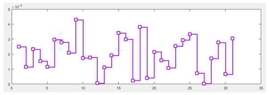
Figure 8. Figure of the relative error.

According to the table and figure above, the forecasting accuracy of the CEEMDAN-MGWO-SVM model is very high, and the relative error of each prediction point is not more than 0.5%.

5.1.4. Comparison of Forecasting Models

To further verify the effectiveness and superiority of the CEEMDAN-MGWO-SVM model proposed in this paper for daily peak load forecasting, we choose the models EEMD-MGWO-SVM, MGWO-SVM, GWO-SVM, SVM and BP neural network to compare with the CEEMDAN-MGWO-SVM model and analyze the forecasting results of the same sample data. The comparison of the forecasting results and the relative errors for different models are shown in Figure 9 and Figure 10, respectively.

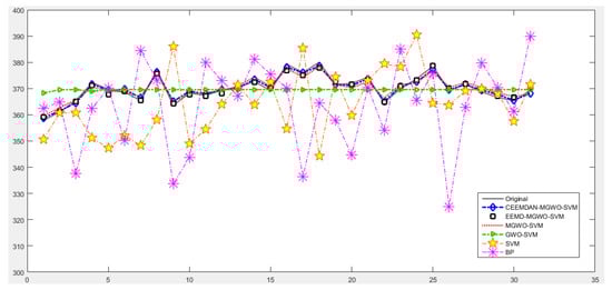
Figure 9. Comparison of forecasting results.

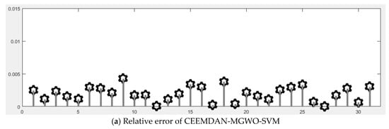
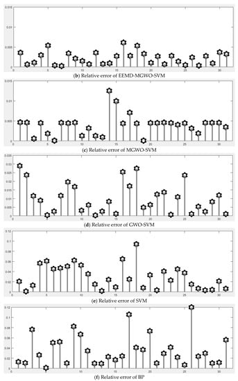
Figure 10. The relative errors of different models: (a) CEEMDAN-MGWO-SVM; (b) EEMD-MGWO-SVM; (c) MGWO-SVM; (d) GWO-SVM; (e) SVM; and (f) BP.

Figure 9 shows the fitting situation of the daily peak load curve predicted by each model and the actual daily peak load curve. Figure 10 shows the relative errors of different models for daily peak load forecasting of S power grid in May 2017. It can be seen that the forecasting curve of the CEEMDAN-MGWO-SVM model in this paper fits best.

To show the forecasting accuracy of each model more intuitively, we use the boxplot to compare the relative errors of each forecasting model. The boxplot displays the following five statistics of the relative error for each forecasting model: the minimum, first quartile, the median, third quartile and the maximum. The boxplot of relative errors for different models are shown in Figure 11.

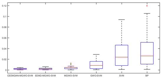
Figure 11. The boxplot of relative errors for different models.

As shown in Figure 10, the relative error of the CEEMDAN-MGWO-SVM model forecasting result is the smallest, followed by EEMD-MGWO-SVM model, and the relative error of BP neural network forecasting result is the largest. The relative errors of the forecasting results for different models are shown in Table 4.

Table 4. The relative errors of the forecasting results for different models.

Date	CEEMDAN-MGWO-SVM	EEMD-MGWO-SVM	MGWO-SVM	GWO-SVM	SVM	BP
1 May 2017	0.2498	0.3587	0.4629	2.8950	2.0416	1.2684
2 May 2017	0.1151	0.0649	0.4581	2.3565	0.0938	1.0711
3 May 2017	0.2329	0.1108	0.0588	1.1474	1.2698	7.6177
4 May 2017	0.1530	0.2952	0.4471	0.8820	5.6522	2.6074
5 May 2017	0.1147	0.5368	0.1813	0.0382	6.0638	0.1083
6 May 2017	0.2962	0.0448	0.0085	0.2563	4.5280	5.0085
7 May 2017	0.2787	0.0261	0.4538	1.1605	4.6686	5.1943
8 May 2017	0.2083	0.3374	0.4399	1.9571	5.0145	1.0076
9 May 2017	0.4294	0.2104	0.4551	1.6746	6.1937	8.2249
10 May 2017	0.1737	0.1493	0.1253	0.3127	5.2642	6.6831
11 May 2017	0.1773	0.0682	0.3164	0.6203	3.5221	3.4118
12 May 2017	0.0065	0.3558	0.1279	0.0368	1.4886	0.9663
13 May 2017	0.1115	0.0771	0.0945	0.2559	0.2047	0.9410
14 May 2017	0.1912	0.0951	1.2521	0.8263	2.3877	2.2650
15 May 2017	0.3413	0.2702	0.9916	0.1156	0.9081	1.6802
16 May 2017	0.2995	0.6088	0.4377	2.5416	6.4518	2.4029
17 May 2017	0.0241	0.2805	0.7071	1.7136	2.4938	10.5361
18 May 2017	0.3804	0.5328	0.4371	2.7351	9.3884	4.0734
19 May 2017	0.0410	0.3300	0.0059	0.4845	0.7985	3.6317
20 May 2017	0.2151	0.1035	0.4445	0.6382	3.2965	7.3358
21 May 2017	0.1574	0.2675	0.4447	1.2408	0.3151	1.0234
22 May 2017	0.1080	0.0713	0.4559	1.3601	4.0552	2.9256
23 May 2017	0.2534	0.2803	0.4487	0.0727	2.2527	4.1116
24 May 2017	0.2935	0.1370	0.4019	1.0860	4.4883	2.1845
25 May 2017	0.3328	0.0469	0.4388	2.3428	3.7140	0.6781
26 May 2017	0.0728	0.2383	0.3126	0.1084	1.5043	11.9655
27 May 2017	0.0035	0.0357	0.1868	0.5341	0.6607	2.3618
28 May 2017	0.1708	0.2708	0.4514	0.2402	0.3170	2.9713
29 May 2017	0.2778	0.0938	0.4529	0.8058	0.4006	1.0120
30 May 2017	0.0660	0.3700	0.4529	1.1853	2.0976	1.1330
31 May 2017	0.3034	0.3215	0.3462	0.1040	0.6086	5.6113

The $MAPE$, $R^2$, $AIC$ and $BIC$ of the forecasting results for the models of CEEMDAN-MGWO-SVM, EEMD-MGWO-SVM, MGWO-SVM, GWO-SVM, SVM and BP neural network are calculated, respectively, as shown in Table 5.

Table 5. Comparison of the forecasting accuracy for different models.

Model	MAPE (%)	${\mathit{R}}^2$ (%)	AIC	BIC
CEEMDAN-MGWO-SVM	0.1961	99.7743	−111.21	−83.47
EEMD-MGWO-SVM	0.2255	99.7240	−74.23	−46.49
MGWO-SVM	0.3967	99.5284	24.38	52.12
GWO-SVM	1.0235	98.6611	216.36	244.10
SVM	2.9724	96.2056	408.03	435.77
BP	3.6133	95.3255	446.41	474.15

As shown in Table 5, the MAPE, $AIC$ and $BIC$ of the CEEMDAN-MGWO-SVM model is the smallest, and the goodness of fit is the best, reaching 99.7743%. Next is the EEMD-MGWO-SVM model, and the goodness of fit is 99.724%. The MAPE, $AIC$ and $BIC$ of BP model is the largest, and the goodness of fit is the worst, reaching 95.3255%. Besides, the prediction effect of MGWO-SVM model is better than that of GWO-SVM, SVM and BP model.

Overall, the evaluation results of the two indexes for different models tend to be consistent. The forecasting accuracy is ranked as follows: CEEMDAN-MGWO-SVM > EEMD-MGWO-SVM > MGWO-SVM > GWO-SVM > SVM > BP.

5.2. Case 2

To fully prove the reliability and universality of the above conclusions, and verify the validity of the CEEMDAN-MGWO-SVM model proposed in this paper for daily peak load forecasting, further experiments are carried out in this paper. In this paper, we select the daily peak load of S power grid from September to November in 2017 as the research object. The daily peak load, daily maximum temperature, daily minimum temperature, daily average temperature, daily average relative humidity, maximum daily wind speed, date type and other data are collected. We use the data from September to October as the training set sample, and the data of November as the test set sample. We choose the models of EEMD-MGWO-SVM, MGWO-SVM, GWO-SVM, SVM and BP neural network to compare with the CEEMDAN-MGWO-SVM model and analyze the forecasting results of the same sample data. The boxplot of relative errors for different models is shown in Figure 12.

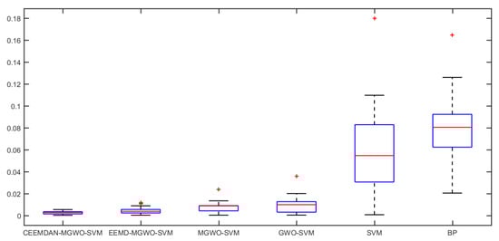
Figure 12. The boxplot of relative errors for different models.

As shown in Figure 12, the relative error of the CEEMDAN-MGWO-SVM model forecasting result is the smallest, followed by EEMD-MGWO-SVM model, and the relative error of BP neural network forecasting result is the largest. The relative errors of the forecasting results for different models are shown in Table 6.

Table 6. The relative errors of the forecasting results for different models.

Date	CEEMDAN-MGWO-SVM	EEMD-MGWO-SVM	MGWO-SVM	GWO-SVM	SVM	BP
1 November 2017	0.0125	0.0566	0.9327	0.2296	9.5773	2.0402
2 November 2017	0.3356	0.2557	0.7723	0.9410	10.9681	9.4039
3 November 2017	0.1775	0.1124	0.9317	1.2614	3.8740	2.1168
4 November 2017	0.3402	0.5767	0.4159	1.0184	17.9909	7.3151
5 November 2017	0.4791	0.5449	0.8286	0.7855	6.8261	2.4805
6 November 2017	0.3690	0.8811	0.9082	1.3103	8.5815	6.2615
7 November 2017	0.1895	0.0999	0.5723	0.2971	10.2695	8.9387
8 November 2017	0.4972	0.4118	0.8980	1.0302	9.7899	10.4270
9 November 2017	0.1386	1.1218	0.8842	1.7575	9.0522	12.0714
10 November 2017	0.0696	0.5363	0.8896	1.6383	5.3297	8.8349
11 November 2017	0.5252	0.3407	0.4491	0.1079	3.9336	5.5385
12 November 2017	0.0786	0.2249	0.0243	0.0884	5.1666	7.1996
13 November 2017	0.1376	0.0315	0.4179	1.2593	7.0206	9.1877
14 November 2017	0.3824	0.1968	0.8952	0.6408	5.9944	8.6280
15 November 2017	0.0953	0.7178	0.2548	0.1638	8.2713	10.5787
16 November 2017	0.4550	1.0708	0.8694	3.5711	8.2825	16.4678
17 November 2017	0.2874	0.3900	0.0910	0.4511	8.1497	9.2269
18 November 2017	0.2512	0.1565	0.8776	0.1707	0.7908	8.7174
19 November 2017	0.1016	1.0934	0.5201	0.8998	3.6849	3.0319
20 November 2017	0.1080	0.4009	0.8945	2.0005	2.4741	4.6025
21 November 2017	0.1566	0.3338	0.8911	1.2727	3.0533	8.0624
22 November 2017	0.3343	0.3630	0.1215	1.1907	7.3540	12.6018
23 November 2017	0.2817	0.3819	0.8792	1.5460	5.5976	8.6934
24 November 2017	0.3019	0.3301	0.2558	1.0565	3.4562	6.6776
25 November 2017	0.2536	0.2511	0.8784	0.1535	2.4492	8.0317
26 November 2017	0.1588	0.0220	0.4242	0.0289	1.4115	6.8785
27 November 2017	0.0253	1.1604	0.1319	1.2607	3.4727	6.2547
28 November 2017	0.3151	0.5443	1.3368	0.7546	0.2483	5.9749
29 November 2017	0.5338	0.4876	1.0956	1.0525	1.2225	9.8106
30 November 2017	0.3020	0.2232	2.3635	0.8789	0.0658	6.2303

The $MAPE$, $AIC$ and $BIC$ of the forecasting results for the models of CEEMDAN-MGWO-SVM, EEMD-MGWO-SVM, MGWO-SVM, GWO-SVM, SVM and BP neural network are calculated, respectively, as shown in Table 7.

Table 7. Comparison of the forecasting accuracy for different models.

Model	MAPE (%)	${\mathit{R}}^2$ (%)	AIC	BIC
CEEMDAN-MGWO-SVM	0.2565	99.7035	−44.03	−16.41
EEMD-MGWO-SVM	0.4439	99.4445	70.23	97.84
MGWO-SVM	0.7235	99.1482	148.02	175.64
GWO-SVM	0.9606	98.7887	212.11	239.73
SVM	5.8119	93.1002	528.75	556.36
BP	7.7428	91.6074	564.39	592.01

As shown in Table 7, the MAPE, $AIC$ and $BIC$ of the CEEMDAN-MGWO-SVM model is the smallest in all models, and the goodness of fit is the best, reaching 99.7035%. Next is the EEMD-MGWO-SVM model, and the goodness of fit is 99.4445%. The MAPE, $AIC$ and $BIC$ of BP model is the largest, and the goodness of fit is the worst, reaching 91.6074%. Besides, the prediction effect of MGWO-SVM model is better than that of GWO-SVM, SVM and BP model. The evaluation results of the two indexes for different models tend to be consistent. The forecasting accuracy is ranked as follows: CEEMDAN-MGWO-SVM > EEMD-MGWO-SVM > MGWO-SVM > GWO-SVM > SVM > BP.

5.3. Case 3

Since the first two cases are both focused on the daily peak load of S power grid, to avoid the contingency of the experimental conclusions, we select the daily peak load of M power grid from March to May 2017 as the research object to do further research. The daily peak load, daily maximum temperature, daily minimum temperature, daily average temperature, daily average relative humidity, maximum daily wind speed, date type and other data are collected. We use the data from March to April as the training set sample, and the data of May as the test set sample. We choose the models of EEMD-MGWO-SVM, MGWO-SVM, GWO-SVM, SVM and BP neural network to compare with the CEEMDAN-MGWO-SVM model and analyze the forecasting results of the same sample data. The boxplot of relative errors for different models is shown in Figure 13.

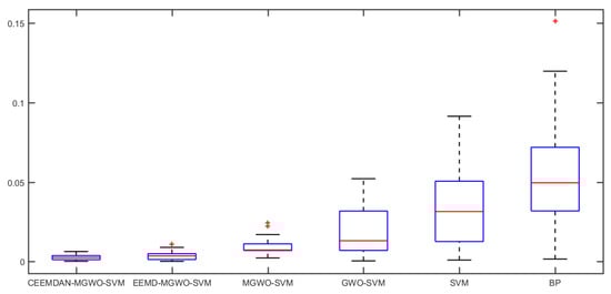
Figure 13. The boxplot of relative errors for different models.

As shown in Figure 13, the relative error of the CEEMDAN-MGWO-SVM model forecasting result is the smallest, followed by EEMD-MGWO-SVM model, and the relative error of BP neural network forecasting result is the largest. The relative errors of the forecasting results for different models are shown in Table 8.

Table 8. The relative errors of the forecasting results for different models.

Date	CEEMDAN-MGWO-SVM	EEMD-MGWO-SVM	MGWO-SVM	GWO-SVM	SVM	BP
1 May 2017	0.0039	1.0913	0.7388	5.2044	6.5708	10.5399
2 May 2017	0.4899	0.3442	0.7289	3.4585	7.3328	10.8552
3 May 2017	0.2762	0.1154	0.7186	1.7216	2.7516	4.9467
4 May 2017	0.1329	0.0294	0.7132	1.2200	7.7586	1.7207
5 May 2017	0.2706	0.0011	0.2151	0.1048	8.0276	3.1361
6 May 2017	0.5786	0.3558	0.7273	3.5182	2.7613	2.1908
7 May 2017	0.1486	0.0876	0.4125	0.6098	3.7143	11.2288
8 May 2017	0.0416	0.6387	0.7019	0.5960	0.4846	8.1817
9 May 2017	0.1008	0.4170	0.6880	2.4228	7.9902	1.8853
10 May 2017	0.3678	0.3389	0.6887	2.0719	1.5935	6.5463
11 May 2017	0.2860	0.2204	1.4484	0.0292	3.7902	8.9700
12 May 2017	0.0739	0.1278	2.2291	1.2994	0.7323	15.1186
13 May 2017	0.1317	0.1029	1.1386	0.6752	5.1811	11.9794
14 May 2017	0.5501	0.7856	0.6968	1.0179	9.1400	5.9361
15 May 2017	0.1929	0.7286	0.6962	0.3853	3.4492	5.6866
16 May 2017	0.4537	0.3585	1.2010	0.9220	1.6169	4.5405
17 May 2017	0.1909	0.1180	0.7064	0.8197	4.6620	4.1317
18 May 2017	0.4783	0.3725	0.6988	0.4312	3.1410	0.1690
19 May 2017	0.2946	0.4490	0.5145	0.1775	0.3118	3.6720
20 May 2017	0.0558	0.0116	0.2316	0.7239	6.7905	5.9620
21 May 2017	0.2459	0.2286	0.9204	0.7644	4.4337	0.1472
22 May 2017	0.3408	0.5379	1.3503	3.3714	3.1462	3.2875
23 May 2017	0.6208	0.8835	1.0075	3.6208	2.3779	4.9723
24 May 2017	0.2611	0.3796	0.6807	2.7356	4.4792	7.2261
25 May 2017	0.0666	0.0179	0.8405	3.3483	1.7718	4.2027
26 May 2017	0.1419	0.2128	0.6749	3.3130	0.0805	6.9585
27 May 2017	0.4845	0.6234	0.6683	3.9371	1.1359	2.4452
28 May 2017	0.3160	0.3023	0.6709	2.4928	0.8866	4.6199
29 May 2017	0.0429	0.1220	1.6882	1.8900	0.8585	7.0703
30 May 2017	0.1883	0.4940	1.3512	2.1488	1.0689	0.6806
31 May 2017	0.0057	0.1657	2.4370	1.1690	1.9454	4.9427

The $MAPE$, $AIC$ and $BIC$ of the forecasting results for the models of CEEMDAN-MGWO-SVM, EEMD-MGWO-SVM, MGWO-SVM, GWO-SVM, SVM and BP neural network are calculated, respectively, as shown in Table 9.

Table 9. Comparison of the forecasting accuracy for different models.

Model	MAPE (%)	${\mathit{R}}^2$ (%)	AIC	BIC
CEEMDAN-MGWO-SVM	0.2527	99.6915	−99.00	−71.26
EEMD-MGWO-SVM	0.3439	99.5631	−34.97	−7.23
MGWO-SVM	0.9092	98.9627	124.14	151.88
GWO-SVM	1.8129	97.7388	267.53	295.27
SVM	3.5479	95.6440	388.17	415.91
BP	5.6113	93.4167	464.16	491.90

As shown in Table 9, the MAPE, $AIC$ and $BIC$ of the CEEMDAN-MGWO-SVM model is the smallest, and the goodness of fit is the best, reaching 99.6915%. Next is the EEMD-MGWO-SVM model, and the goodness of fit is 99.5631%. The MAPE, $AIC$ and $BIC$ of BP model is the largest, and the goodness of fit is the worst, reaching 93.4167%. Besides, the prediction effect of MGWO-SVM model is better than that of GWO-SVM, SVM and BP model. The evaluation results of the two indexes for different models tend to be consistent. The forecasting accuracy is ranked as follows: CEEMDAN-MGWO-SVM > EEMD-MGWO-SVM > MGWO-SVM > GWO-SVM > SVM > BP.

5.4. Analysis of Empirical Results

According to the experimental results of the above three cases, the ranking of the forecasting accuracy for each model tends to be consistent and the forecasting accuracy of the CEEMDAN-MGWO-SVM model is significantly higher than other models, which proves that the CEEMDAN-MGWO-SVM model proposed in this paper is practical and effective for daily peak load forecasting.

Through the comparison and analysis of the experimental results, we found that:

(1)

Daily peak load is susceptible to festival factors and meteorological factors such as daily maximum temperature, daily minimum temperature, daily average temperature, daily average relative humidity and maximum daily wind speed, which present certain volatility. Doing the operation of signal decomposition-forecasting-reconstruction for the original daily peak load sequence can obtain the higher accuracy forecasting results compared with direct prediction.

(2)

Adding the adaptive white noise to improve the EEMD algorithm can effectively eliminate the chaos of the original data and reduce the noise of the daily peak load sequence.

(3)

Using the combined model for forecasting can achieve complementary advantages between different algorithms, which greatly improves the forecasting accuracy.

The CEEMDAN-MGWO-SVM model proposed in this paper realizes noise reduction for non-stationary daily peak load sequence by complete ensemble empirical mode decomposition with adaptive noise, which makes the daily peak load sequence more regular. The model adopts the grey wolf optimization algorithm, which is improved by introducing the population dynamic evolution operator and the nonlinear convergence factor to enhance the global search ability and avoid falling into the local optimum, thus can better optimize the parameters of the SVM algorithm. The CEEMDAN-MGWO-SVM model greatly improves the forecasting accuracy of daily peak load and shows the powerful generalization ability and robustness.

6. Conclusions

A novel daily peak load forecasting model, CEEMDAN-MGWO-SVM, is proposed in this paper. Firstly, the model uses the complete ensemble empirical mode decomposition with adaptive noise (CEEMDAN) algorithm to decompose the daily peak load sequence into multiple sub-sequences. Then, the model of modified grey wolf optimization and support vector machine (MGWO-SVM) is adopted to forecast the sub-sequences. Finally, the forecasting sequence is reconstructed and the forecasting result is obtained. Using CEEMDAN can realize noise reduction for non-stationary daily peak load sequence, which makes the daily peak load sequence more regular. The model adopts the grey wolf optimization algorithm, which is improved by introducing the population dynamic evolution operator and the nonlinear convergence factor to enhance the global search ability and avoid falling into the local optimum, thus can better optimize the parameters of the SVM algorithm for improving the forecasting accuracy of daily peak load. In this paper, three cases are used to test the forecasting accuracy of the CEEMDAN-MGWO-SVM model. We choose the models EEMD-MGWO-SVM, MGWO-SVM, GWO-SVM, SVM and BP neural network to compare with the CEEMDAN-MGWO-SVM model and analyze the forecasting results of the same sample data. The experimental results fully demonstrate the reliability and effectiveness of the CEEMDAN-MGWO-SVM model proposed in this paper for daily peak load forecasting, which shows the strong generalization ability and robustness of the model.

References

- Lee, W.J.; Hong, J. A hybrid dynamic and fuzzy time series model for mid-term power load forecasting. Int. J. Electr. Power Energy Syst. 2015, 64, 1057–1062. [Google Scholar] [CrossRef]
- Chikobvu, D.; Sigauke, C. A frequentist and Bayesian regression analysis to daily peak electricity load forecasting in South Africa. Afr. J. Bus. Manag. 2012, 6, 10524–10533. [Google Scholar] [CrossRef]
- Guo, L.; Jiang, D.; Liu, Y.; Ren, L.; Yang, F.; Li, J.; Wang, B.; State Grid Sichuan Electric Power Company; State Grid Deyang Power Supply Company; State Grid Aba Power Supply Company; School of Electrical Engineering, Wuhan University. Medium and Long-term Load Forecasting Based on Adaptive Weight Buffer Gray Theory. Shaanxi Electr. Power 2016, 44, 33–37. [Google Scholar]
- Wang, W.C.; Kwokwing, C.; Cheng, C.T.; Qiu, L. A comparison of performance of several artificial intelligence methods for forecasting monthly discharge time series. J. Hydrol. 2009, 374, 294–306. [Google Scholar] [CrossRef]
- Jurasz, J. Day ahead electric power load forecasting by WT-ANN. Prz. Elektrotech. 2016, 1, 154–156. [Google Scholar] [CrossRef]
- Xiao, Z.; Ye, S.J.; Zhong, B.; Sun, C.X. BP neural network with rough set for short term load forecasting. Expert Syst. Appl. 2009, 36, 273–279. [Google Scholar] [CrossRef]
- Zhaoyu, P.; Li, S.; Zhang, H.; Zhang, N. The Application of the PSO Based BP Network in Short-Term Load Forecasting. Phys. Procedia 2012, 24, 626–632. [Google Scholar] [CrossRef]
- Wang, J.J.; Shi, P.; Jiang, P.; Hu, J.W.; Qu, S.; Chen, X.; Chen, Y.; Dai, Y.; Xiao, Z. Application of BP Neural Network Algorithm in Traditional Hydrological Model for Flood Forecasting. Water 2017, 9, 48. [Google Scholar] [CrossRef]
- Huang, D.Z.; Gong, R.X.; Gong, S. Prediction of Wind Power by Chaos and BP Artificial Neural Networks Approach Based on Genetic Algorithm. J. Electr. Eng. Technol. 2015, 10, 41–46. [Google Scholar] [CrossRef]
- Narayanakumar, S.; Raja, K. A BP Artificial Neural Network Model for Earthquake Magnitude Prediction in Himalayas, India. Circuits Syst. 2016, 7, 3456–3468. [Google Scholar] [CrossRef]
- Pai, P.F.; Hong, W.C. Support vector machines with simulated annealing algorithms in electricity load forecasting. Energy Convers. Manag. 2005, 46, 2669–2688. [Google Scholar] [CrossRef]
- Hong, W.C. Electric load forecasting by support vector model. Appl. Math. Model. 2009, 33, 2444–2454. [Google Scholar] [CrossRef]
- Nie, H.; Liu, G.; Liu, X.; Wang, Y. Hybrid of ARIMA and SVMs for Short-Term Load Forecasting. Energy Procedia 2012, 16, 1455–1460. [Google Scholar] [CrossRef]
- Wei, L.; Zhao, F.; Wang, S. Short-term power load forecasting of support vector machine based on parameters optimization of population search algorithm. Electr. Meas. Instrum. 2016, 53, 45–49. [Google Scholar]
- Sun, Y.; Leng, B.; Guan, W. A novel wavelet-SVM short-time passenger flow prediction in Beijing subway system. Neurocomputing 2015, 166, 109–121. [Google Scholar] [CrossRef]
- Shi, X.; Huang, J.; Chang, J.; Wang, J.; Zhao, J. Optimal parameters of the SVM for temperature prediction. Proc. Int. Assoc. Hydrol. Sci. 2015, 368, 162–167. [Google Scholar] [CrossRef]
- Huang, C.L.; Dun, J.F. A distributed PSO–SVM hybrid system with feature selection and parameter optimization. Appl. Soft Comput. 2008, 8, 1381–1391. [Google Scholar] [CrossRef]
- Liu, Q.; Huang, Z. Research on power load forecasting models based on simulated annealing support vector machine (SA-SVM) algorithm mathematical. Metall. Min. Ind. 2015, 9, 924–929. [Google Scholar]
- Wang, J.; Ran, R.; Song, Z.; Sun, J. Short-Term Photovoltaic Power Generation Forecasting Based on Environmental Factors and GA-SVM. J. Electr. Eng. Technol. 2017, 12, 64–71. [Google Scholar] [CrossRef]
- Mirjalili, S.; Mirjalili, S.M.; Lewis, A. Grey Wolf Optimizer. Adv. Softw. Eng. 2014, 69, 46–61. [Google Scholar] [CrossRef]
- Mirjalili, S.; Saremi, S.; Mirjalili, S.M.; Coelhod, L.D.S. Multi-objective grey wolf optimizer: A novel algorithm for multi-criterion optimization. Expert Syst. Appl. 2016, 47, 106–119. [Google Scholar] [CrossRef]
- Turabieh, H. A Hybrid ANN-GWO Algorithm for Prediction of Heart Disease. Am. J. Oper. Res. 2016, 6, 136–146. [Google Scholar] [CrossRef]
- Xu, D.Y.; Ding, S. Research on improved GWO-optimized SVM-based short-term load prediction for cloud computing. Comput. Eng. Appl. 2017, 53, 68–73. [Google Scholar]
- Benaouda, D.; Murtagh, F.; Starck, J.L.; Renaudd, O. Wavelet-based nonlinear multiscale decomposition model for electricity load forecasting. Neurocomputing 2006, 70, 139–154. [Google Scholar] [CrossRef]
- Xiang, Z.R.; Wang, X.P. Forecasting Approach to Short-time Load Using Wavelet Decomposition and Artificial Neural Network. J. Syst. Simul. 2008, 20, 5018–5020. [Google Scholar]
- Fei, S.W.; He, Y. Wind speed prediction using the hybrid model of wavelet decomposition and artificial bee colony algorithm-based relevance vector machine. Int. J. Electr. Power Energy Syst. 2015, 73, 625–631. [Google Scholar] [CrossRef]
- Seo, Y.; Kim, S.; Kisi, O.; Singhd, V.P. Daily water level forecasting using wavelet decomposition and artificial intelligence techniques. J. Hydrol. 2015, 520, 224–243. [Google Scholar] [CrossRef]
- Huang, N.E. A Study of the Characteristics of White Noise Using the Empirical Mode Decomposition Method. Proc. R. Soc. A 2004, 460, 1597–1611. [Google Scholar] [CrossRef]
- Sha, F.; Zhu, F.; Guo, S.N.; Gao, J.T. Based on the EMD and PSO-BP Neural Network of Short-Term Load Forecasting. Adv. Mater. Res. 2013, 614–615, 1872–1875. [Google Scholar] [CrossRef]
- Zheng, H.; Yuan, J.; Chen, L. Short-Term Load Forecasting Using EMD-LSTM Neural Networks with a Xgboost Algorithm for Feature Importance Evaluation. Energies 2017, 10, 1168. [Google Scholar] [CrossRef]
- Premanode, B.; Toumazou, C. Improving prediction of exchange rates using Differential EMD. Expert Syst. Appl. 2013, 40, 377–384. [Google Scholar] [CrossRef]
- Wang, T.; Zhang, M.; Yu, Q.; Zhang, H. Comparing the application of EMD and EEMD on time-frequency analysis of seimic signal. J. Appl. Geophys. 2012, 83, 29–34. [Google Scholar] [CrossRef]
- Liu, Z.; Sun, W.; Zeng, J. A new short-term load forecasting method of power system based on EEMD and SS-PSO. Neural Comput. Appl. 2014, 24, 973–983. [Google Scholar] [CrossRef]
- Jiang, X.; Zhang, L.; Chen, X. Short-term forecasting of high-speed rail demand: A hybrid approach combining ensemble empirical mode decomposition and gray support vector machine with real-world applications in China. Transp. Res. Part C Emerg. Technol. 2014, 44, 110–127. [Google Scholar] [CrossRef]
- Colominas, M.A.; Schlotthauer, G.; Torres, M.E. Improved complete ensemble EMD: A suitable tool for biomedical signal processing. Biomed. Signal Process. Control 2014, 14, 19–29. [Google Scholar] [CrossRef]
- Helske, J.; Luukko, P. Ensemble Empirical Mode Decomposition (EEMD) and Its CompleteVariant (CEEMDAN). Int. J. Public Health 2015, 60, 1–9. [Google Scholar]
- Zhang, W.; Qu, Z.; Zhang, K.; Mao, W.; Ma, Y.; Fan, X. A combined model based on CEEMDAN and modified flower pollination algorithm for wind speed forecasting. Energy Convers. Manag. 2017, 136, 439–451. [Google Scholar] [CrossRef]
- Jun, L.I.; Qing, L.I. Medium term electricity load forecasting based on CEEMDAN-permutation entropy and ESN with leaky integrator neurons. Electr. Mach. Control 2015, 19, 70–80. [Google Scholar] [CrossRef]
© 2018 by the authors. Licensee MDPI, Basel, Switzerland. This article is an open access article distributed under the terms and conditions of the Creative Commons Attribution (CC BY) license (http://creativecommons.org/licenses/by/4.0/).