Abstract
Short-term wind power forecasting is a technique which tells system operators how much wind power can be expected at a specific time. Due to the increasing penetration of wind generating resources into the power grids, short-term wind power forecasting is becoming an important issue for grid integration analysis. The high reliability of wind power forecasting can contribute to the successful integration of wind generating resources into the power grids. To guarantee the reliability of forecasting, power curves need to be analyzed and a forecasting method used that compensates for the variability of wind power outputs. In this paper, we analyzed the reliability of power curves at each wind speed using logistic regression. To reduce wind power forecasting errors, we proposed a short-term wind power forecasting method using support vector machine (SVM) based on linear regression. Support vector machine is a type of supervised leaning and is used to recognize patterns and analyze data. The proposed method was verified by empirical data collected from a wind turbine located on Jeju Island.
1. Introduction
Wind power generation has grown rapidly over the past few decades, as demonstrated by the total accumulated wind power capacity which hit 319 GW from an installation in 2013 [1]. Furthermore, the worldwide total of wind power capacity was 432.9 GW in 2015, showing that the cumulative market of wind power grew more than 17%, with wind power capacity expected to increase consistently, to the point where wind power will generate 4337 TWh in 2035 [1,2]. For this reason, wind power forecasting—a technique that determines the quantity of wind power output that can be expected over a given period—is becoming a salient point of research as an important component in operating power systems to maintain their reliability.
Prior to forecasting wind power outputs, power curves need to be analyzed as they represent characters of wind turbine outputs. There are few studies on the reliability of power curves using regression and artificial neural network models, etc. [3]; therefore, we have analyzed the reliability of a power curve at each wind speed through the wind turbine’s power curve, and output the data using a logistic regression. In statistics, a logistic regression measures the relationship between a categorical dependent variable and one or more independent variables by estimating probabilities based on a logistic function, which is the cumulative logistic distribution [4]. Using a logistic regression, wind power outputs can be distributed (which do or do not enter the error range) at each wind speed, to create a probability model relating to the reliability of power curves.
Accurate wind power forecasting is essential when it comes to considering variability, reducing uncertainty, and penetrating wind power into power systems. Wind power forecasting is largely divided into three parts based on time horizon: short-term (one hour to one day), medium-term (one day to one week), and long-term (one week to one year) [5]. In particular, given the increasing supply of wind-generated power into the power grid, short-term wind power forecasting is becoming a critical issue in the safe operation of power systems. Precise short-term wind power forecasting can enable efficient power system management, improve the wind power supply level, and increase overall systemic reliability. Additionally, it can be utilized for power system planning such as unit commitment and dispatch scheduling [6]. Many approaches for predicting wind power have been proposed to increase the reliability of forecasted values. For wind power forecasting, there are models based on time series using auto regression moving average (ARMA)/auto regression integrated moving average (ARIMA), or the regression method [7]. These methods have many advantages: they can forecast fast and do not need many elements to forecast. However, time series models need lots of data when the model is structured, and the parameters are difficult to update when new data are uploaded. Furthermore, the regression model has limits in containing patterns and the variability of data.
Recently, many advanced approaches have been suggested to forecast more exact wind power outputs based on statistic and ensemble methods [8,9,10,11]. In this study, we proposed the use of support vector machine (SVM) to forecast wind power outputs. SVM is one of the most popular models in the field of machine learning [12], and is an advanced technique for classification and regression analysis. The support vector regression (SVR) is the method with which to carry out a SVM [13] based on regression as this model can consider variability as SVM is not largely influenced by noise data, which gives the high accuracy [14]. In this paper, we analyzed the accuracy of power curves at each wind speed using logistic regression, and also proposed short-term wind power forecasting using support vector machine based on linear regression to reduce wind power forecasting errors. To achieve this, we used the value of the power curve at each speed, and the accuracy of the power curve was calculated using logistic regression as additional variables. These variables are able to compensate when the forecasted wind speeds input had uncertainty. For this reason, it was possible to improve the error caused by the sudden change of output. In Section 2, the mathematical theories about logistic regression and SVM are described. In Section 3 and Section 4, we analyze the accuracy of the power curve using logistic and forecast wind power outputs through the SVM method. In Section 5, we summarize the results of this research.
2. Mathematical Definition for Enhanced Reliability Assessments Method of Wind Turbines
2.1. Logistic Regression
Logistic regression analysis is applicable to data that do not follow the normal distribution. Using logistic regression analysis, it is possible to interpret discrete data which could not be analyzed by linear regression analysis.
Simple linear regression is a statistical method used for predicting and analyzing an independent variable that is influenced by a dependent variable when a dependent variable is continuous [15]. Since dependent variables are binary and not continuous, it is impossible to use simple linear regression. In simple linear regression, the interaction formula between a dependent variable, Y, and an independent variable, X, is assumed in the linear model as:
Here, the dependent variable and independent variables are continuous variables. In this regression model, is an observation’s expectation, and is the error where the independent variable, X, is . The expectation is assumed to be the independent variable’s linear expression. The error, , follows the lognormal distribution as wind speed cannot have negative values, and this parameter can be zero, if it is assumed to be unbiased. , which is consistent irrespective of , has an average zero as the center. Errors and occur independently (). For example, we could define as follows:
In this assumption, is the realization of a random variable . If we apply the variable which has a rate of success , to a simple linear regression, we can get a regression model as follows:
We can then calculate an expected value when X is expressed by :
In this equation, we can determine that the expected value is represented as a probability when the independent variable, X, is . At this point, we can encounter problems with using a simple linear regression for analyzing binary data. First, the error term does not follow a normal distribution. When is a binary dependent variable, the error term, , has two values, ( and (. The second problem is that a simple linear regression has expectations between and . However, if we apply binary data to a simple linear regression, then expectations always have values between 0 and 1. Therefore, this model is inadequate for applying a simple linear regression to binary variables.
We can make a rule or classification which guesses the binary output from input variables. Due to classification, the dependent variable will have binary variables, and the expectation, , will represent a probability which has values between 0 and 1. Therefore, the dependent variable would be a binary variable, so it can be sufficient to use in a curve model, but not a linear model. The typical curve model is a logistic model [16] expressed by Equation (5):
where is an observation’s expectation, , which is a curve model. The logistic model is used to estimate the probability of a binary response. Here, the logistic regression measures the relationship between a categorical dependent variable and one or more independent variables by estimating probabilities through a logistic model [17].
We can transform the logistic model into a linear model. This can be expressed as follow:
This transformation is called a logit transformation, which is defined by , where is a proportion.
This mode of logistic regression [18] uses the method of maximum likelihood estimation for estimating a regression coefficient. Here, the maximum likelihood estimation is a method for estimating a population parameter using a value which maximizes a likelihood function. The likelihood function is represented by a sample and population function.
Assume that , for some function, p, parameterized by , which is itself parameterized function. When observations comprise independent variables, the likelihood function is expressed by Equation (7):
The probability sampling, , is estimated by a sequence of Bernoulli trials, which is represented by :
If each trial were to have its own probability of success, , the likelihood would be expressed by Equation (9):
Equation (9) shows that the likelihood is the same as the probability sample’s joint probability function.
In this logistic regression [19], analyzing the regression coefficient is difficult as the regression model is not linear. Therefore, we need to utilize the odds’ conception for understanding a regression coefficient.
Suppose the numerical values between 0 and 1 are allocated two outcomes of a binary variable. The 0 signifies a negative response and 1 signifies a positive response. When is the ratio of observations with an outcome of 1, then 1 − is the ratio of an outcome of 0. This proportion is called the odds which is represented by Equation (10):
When the probability of success is higher than the probability of failure, the odds has a value greater than 1. Otherwise, when the probability of failure is higher than the probability of success, the odds has a value less than 1.
In logistic regression [20], the regression model uses log odds, which involves applying the natural logarithm to odds. When we assume that the prediction probability is , we can estimate the log odds as follow:
If we were to use an exponential function on either side, we can generate transformed odds, as in the Equation (12):
In this equation, the odds’ predicted value is multiplied as much as . If is 0, then the intercept, , becomes a predicted value.
2.2. Support Vector Regression (SVR)
As discussed in Section 1, support vector machine (SVM) is one of the most popular models in the field of machine learning and is an advanced technique for classification and regression analysis. SVM is not largely influenced by noise data and has high accuracy; furthermore, this model is easier to use than other machine learning approaches [21], and has been used for wind power forecasting [22]. Typically, the basis for training appropriate model is represented as follows:
where denotes the space of the input patterns; the dataset, D, consists of labeled patterns; K signifies discrete space and indicates in regression scenarios. The purpose of this learning process is to find a prediction function, “”, to map hidden patterns to reasonable labels with real values. We can formulate the time series data which are measured outputs at time . Measured outputs are defined D in Equation (13).
To extend the SVM [21] to cases for which the data is not linearly separable, we use a hinge loss function, as follows:
This function is zero if the constraint is satisfied. This constraint is represented as:
In Equations (2) and (3), are either 1 or −1, each indicating the class to which the point —a p-dimensional real vector—belongs. In addition, is the normal vector to the hyperplane and indicates the correct side of the margin [19]. For data on the incorrect side of the margin, the function’s value is relative to the distance from the margin. Therefore, we need to minimize the loss function, as follows:
where λ indicates the decision to swap between increasing the margin size and ensuring that resides on the correct side of the margin. Thus, for thoroughly small values of λ, the soft-margin SVM will still learn a viable categorization rule [22,23].
The SVR is a method to carry out a SVM based on regression. The SVR is divided into three types: a linearly separable SVR, a linearly inseparable SVR, and a nonlinear SVR [24].
In this paper, a nonlinear SVR was used to forecast wind power outputs. To do so, we used historical data for wind power output and wind speed data for training, in addition to the power curve’s value and accuracy data for correcting errors.
3. Reliability of Power Curve Estimation Using Logistic Regression
As discussed in Section 1, the power curves first need to be analyzed as they represent the character of a wind turbine’s outputs. In this section, we describe the construction of a statistical model to estimate the reliability of power curves, based on logistic regression using R language version 3.3.1. Wind power outputs and wind speeds, which were measured in single turbine from Jeju Island, were used as data as one minute averaged values. We constructed one minute data into 10 min and one hour averaged data by averaging 10 and 60 data of one minute. Wind speeds were measured by nacelle. The turbine was made by the HANJIN Industry Corporation (Seoul, Korea), model number HJWT2000, with a capacity of 2000 kW.
3.1. Jeju Island’s Empirical Output Data and Power Curve from Manufacturer
To perform this estimation, we used outputs measured from November to December 2015 from Jeju Island (the corresponding area is not specified to protect the security of the technical data).
Since the reliability analysis of the output curve must be performed prior to the output prediction, the data before the predicted data were used. Figure 1 represents the turbine’s power curve from the manufacturer and the measured outputs. As power curves normally contain a mean power value over 10 min, we constructed a power curve by converting one minute of data to 10 min of data using the average method.
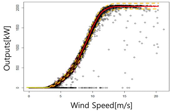
Figure 1.
The wind turbine’s power curve from the manufacturer (red line), ±20% of the power curve’s values (orange dashed lines) and measured outputs (black circles) from a wind turbine located on Jeju Island.
As the power curve from the manufacturer did not correspond with the measured output data, we suggested a logistic regression to estimate the reliability of the power curve.
3.2. Classify Output Data Based on the Power Curve
To generate a logistic regression, we classified output data based on the power curve from the manufacturer. The classification was decided by whether the outputs were included in the ±20% of the power curve’s values at each wind speed or not. The band of classification is represented by dashed lines in Figure 1. In reality, as power curves frequently include a ±20% variability of measured power output [22], we classified the outputs into two categories, by error, based on whether the output data existed within the ±20% variability. We determined that the outputs were within the assumed existing error range throughout the entire range.
3.3. Reliability of Power Curve Estimation
After classification, we obtained values of 1 and 0, which is represented in Figure 2.
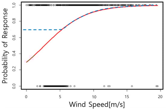
Figure 2.
The statistical model for estimating reliability of power curves using logistic regression (The red line is statistical model and the blue line is fixed minimum value).
As seen in Figure 2, the classified data was non-linear and binary which meant that we could not use a linear regression model to analyze the data. Therefore, to analyze the binary data, which had a non-linear character, we used a logistic regression that could analyze non-linear data to make a statistical model. This model (represented by the red line) was used for estimating the reliability of a power curve from the manufacturer based on logistic regression. The band of ±20% variability got narrower while wind speed decreased, and would tend to be zero when the cut-in speed was approached. Wind measurement errors do not reduce proportionally to wind speed, so power curve reliability for low wind speeds could be underestimated. For this reason, we fixed the minimum value so that when the wind goes under a value (6 m/s), which is represented by the blue dashed line. The “X” label signifies wind speed, and the “Y” label signifies the probability that outputs exist within a tolerance band. Using this statistical model, we could estimate the reliability of a power curve at each wind speed. This is represented in Table 1.

Table 1.
The probability that outputs exist within a tolerance band.
We estimated the reliability of the power curve at each wind speed using this statistical model (Figure 2), which was deduced by logistic regression.
4. Wind Power Forecasting by Using SVR
As discussed in Section 2, we used a SVM based on a multi-variable regression to forecast wind power outputs [25]. Before any actual wind power forecasting, we analyzed Jeju Island’s output data and independent variables, and used the empirical data including wind power outputs, wind speed, power curve’s value and accuracy for training the SVM and forecasting wind power outputs.
4.1. Analysis of Empirical Data
To perform the wind power forecasting, we use outputs measured in January, 2016 from Jeju Island.
As seen in Figure 3, the wind power outputs were highly variable. To forecast wind power outputs, we considered three independent variables: wind speed, the value of the power curve at each speed, and the accuracy of the power curve. The forecasting of wind power outputs was progressed through the process as seen in Figure 4. The accuracy of the turbine’s power curve was calculated by applying the wind speed, outputs, and turbine’s power curve data to logistic regression analysis. The accuracy of the power curve was used as an auxiliary variable for the correction of the error. After forecasting the accuracy of the power curve, SVM model training was performed using the weekly data of wind speed, power, power curve, and power curve accuracy. Through training, the model analyzed patterns between past data, and when input data arrived, the model would derive results through the pattern learning result. In this paper, the forecasted wind velocity was used as the input data to perform the output forecast.
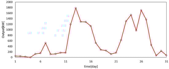
Figure 3.
Wind power outputs from Jeju Island in January 2016.
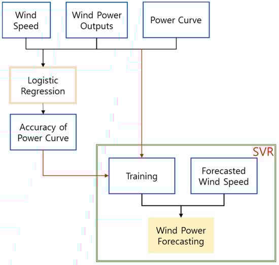
Figure 4.
The process of wind power forecasting using logistic regression and SVR (support vector regression) method.
If a single variable is considered, it is possible for a large error to occur when a wrong single variable enters the input data. Therefore, there is a need to consider multi-variables. We used the value of the power curve at each speed and the accuracy of power curve, which is calculated by using logistic regression as additional variables. These variables compensate when there is uncertainty in the input of forecasted wind speeds.
4.2. Jeju Island’s Wind Power Outputs Forecasting
The training period was seven days long as learning periods can become biased towards past data. After training, we forecasted wind power outputs after 24 h, for the month of January 2016. In all cases, the results were slightly improved, but it was difficult to represent all days. Therefore, the two best cases were selected. In this case, we used historical data measured from 1 to 7 January 2016 from Jeju Island to train the SVM using R language and the “e1071” package [26,27,28]. After training, we forecasted wind power outputs for 8 January. The SVR model parameters are represented in Table 2.
Table 2.
SVR model parameter for forecasting wind power outputs on 8 January 2016.
The parameters of the SVR model listed in Table 2 were constructed through training using data from 1 to 7 January 2016. By applying these parameters, we forecasted wind power outputs for 8 January 2016. The results are in Figure 5. As shown in Figure 5, forecasted values using the SVR model and the proposed method (using the SVR model based on multi variables) were similar to the measured values. Both the SVR model and SVM based on multi-variable regression were highly accurate.
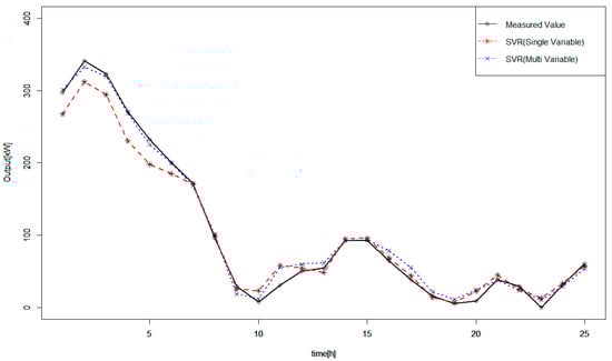
Figure 5.
Measured and forecasted wind power outputs on 8 January 2016.
Table 3 shows the accuracy of the forecasted output values. Both forecasting methods exhibited high accuracy, but the proposed method was more accurate. In Figure 5, we used historical data measured from 4 to 10 January 2016 from Jeju Island, to train the SVM. After training, we forecasted wind power outputs for 11 January (The forecasted values are added to Appendix A).
Table 3.
Accuracy of SVR model and Persistence method (8 January 2016).
The SVR model parameters (which were set for forecasting wind power outputs on 11 January 2016) are represented in Table 4.
Table 4.
SVR model parameter for forecasting wind power outputs on 11 January 2016.
The parameters listed in Table 5 are the parameters of the SVR model constructed through training using data from 4 to 10 January 2016. By applying these parameters, we forecasted wind power outputs for 11 January 2016. The results are shown in Figure 6.
Table 5.
Accuracy of SVR model and Persistence method (11 January 2016).
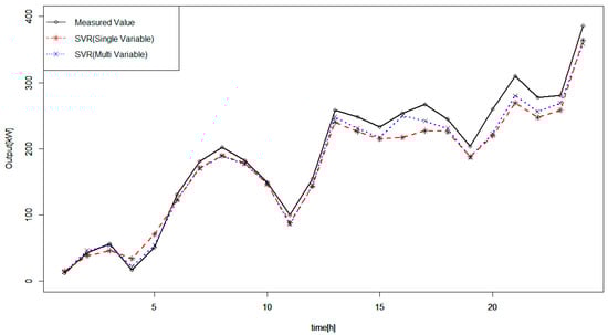
Figure 6.
Measured and forecasted wind power outputs on 11 January 2016.
In Figure 6, the measured values are represented with a black line; forecasted values using the SVR model based on wind power outputs and wind speed are represented as a red line; and forecasted values based on the proposed method are represented with a blue line (The forecasted values are added to Appendix A). Both forecasting models exhibited high accuracy, but the proposed method generated more accurate forecast values.
To confirm this performance numerically, we calculated correlation, R-squared, and RMSE. Table 5 represents the accuracy of that forecasted output values.
5. Conclusions
Short-term wind power forecasting is an important technique as it can inform system operators of how much wind power can be expected at a specific time. To increase the penetration of wind generating resources into the power grids, short-term wind power forecasting is becoming an important issue for grid integration analysis. To guarantee the reliability of forecasting, power curves need to be analyzed, and a forecasting method selected which compensates for the variability of wind power outputs. In this paper, we proposed an enhanced reliability assessment of power curves at each speed using logistic regression as the outputs predicted by the power curve and wind speed were accurate using this estimated reliability. Support vector machine is a kind of supervised learning and is a method for recognizing patterns and analyzing data; therefore, we proposed a method for forecasting wind power outputs using an SVM based on multi-variable regression to increase reliability.
The proposed method was verified with empirical data from a wind turbine located on Jeju Island. We used limited data and one wind turbine size. These limitations can be improved when additional data are available. We considered historical data including wind power output, wind speed, power curve, and the accuracy of the power curve for training. During training, the purpose of the power curve and its accuracy were made by correcting errors. After training, we forecasted wind power outputs over the next 24 h. We obtained the forecasted values by using a SVM based on a multi-variable regression, which was more accurate than the SVM based on single-variable regression (A review of additional turbines is summarized in Appendix A). Thus, the proposed method for estimating accuracy and forecasting outputs can provide reliable predictions of wind power outputs to power system operators.
Acknowledgments
This work was supported by the Korea Institute of Energy Technology Evaluation and Planning (KETEP) and the Ministry of Trade, Industry & Energy (MOTIE) of the Republic of Korea (No. 20161210200560).
Author Contributions
Jin Hur conceived and designed the overall research; BeomJun Park developed the accurate short-term power forecasting model and conducted the experimental simulation; Jin Hur and BeomJun Park wrote the paper; and Jin Hur guided the research direction and supervised the entire research process.
Conflicts of Interest
The authors declare no conflict of interest.
Appendix A
Table A1 shows the forecasted values based on those represented in Figure 5. Wind power forecasting using a SVM based on a multi-variable regression model was more accurate than forecasting using a SVM based on a single-variable regression model.
Table A1.
Measured and forecasted wind power outputs on 8 January 2016.
Table A1.
Measured and forecasted wind power outputs on 8 January 2016.
| Hour | Measured [kW] | SVR (Single Variables) [kW] | SVR (Multi Variable) [kW] |
|---|---|---|---|
| 1 | 296.9598 | 267.4591 | 300.9246 |
| 2 | 341.4116 | 312.1750 | 332.6964 |
| 3 | 323.0441 | 294.2303 | 319.6960 |
| 4 | 271.0491 | 230.3204 | 268.9342 |
| 5 | 232.4090 | 197.8502 | 225.4609 |
| 6 | 199.9801 | 185.1180 | 199.5423 |
| 7 | 171.8569 | 170.9805 | 168.4929 |
| 8 | 95.5342 | 99.6494 | 100.8628 |
| 9 | 29.3689 | 25.4090 | 18.6278 |
| 10 | 7.5669 | 23.0390 | 11.4897 |
| 11 | 30.6104 | 58.0121 | 55.5026 |
| 12 | 50.0074 | 54.4576 | 59.8538 |
| 13 | 54.6308 | 48.3745 | 61.4500 |
| 14 | 92.1981 | 95.0139 | 92.6552 |
| 15 | 93.1122 | 95.7353 | 94.0444 |
| 16 | 64.3447 | 68.4379 | 78.6010 |
| 17 | 38.1156 | 43.8451 | 55.2460 |
| 18 | 15.6717 | 13.7728 | 21.5177 |
| 19 | 5.7529 | 6.9873 | 11.3017 |
| 20 | 8.7146 | 22.3561 | 24.5019 |
| 21 | 38.1685 | 44.7369 | 37.8291 |
| 22 | 29.4539 | 25.2614 | 23.6915 |
| 23 | 0.0000 | 12.8945 | 10.0190 |
| 24 | 31.5425 | 33.3151 | 29.0014 |
Table A2 shows the forecasted values based on those shown in Figure 6. Unsurprisingly, wind power forecasting using a SVM based on a multi-variable regression model was more accurate. Again, we calculated correlation, R-squared, and RMSE to confirm the accuracy numerically.
Table A2.
Measured and forecasted wind power outputs on 11 January 2016.
Table A2.
Measured and forecasted wind power outputs on 11 January 2016.
| Hour | Measured [kW] | SVR (Single Variable) [kW] | SVR (Multi Variables) [kW] |
|---|---|---|---|
| 1 | 11.8804 | 15.1721 | 14.6157 |
| 2 | 43.2991 | 38.5229 | 46.7491 |
| 3 | 56.2944 | 46.1228 | 54.6041 |
| 4 | 16.8877 | 34.2175 | 22.3426 |
| 5 | 51.2966 | 70.6714 | 55.3924 |
| 6 | 130.8975 | 123.2936 | 123.3551 |
| 7 | 180.7022 | 171.4096 | 171.4022 |
| 8 | 201.9767 | 189.8895 | 189.9328 |
| 9 | 182.3402 | 178.1740 | 177.7160 |
| 10 | 149.3459 | 146.7730 | 147.3944 |
| 11 | 100.2452 | 87.8356 | 86.8331 |
| 12 | 154.6401 | 144.0491 | 144.8370 |
| 13 | 258.8261 | 240.4598 | 249.1183 |
| 14 | 247.9340 | 226.3591 | 231.6409 |
| 15 | 233.1442 | 214.8088 | 217.2803 |
| 16 | 253.4962 | 217.0605 | 250.0018 |
| 17 | 267.1652 | 227.2595 | 242.8441 |
| 18 | 244.9381 | 225.9953 | 231.6946 |
| 19 | 203.7053 | 187.9981 | 187.2971 |
| 20 | 259.7748 | 220.0076 | 223.5598 |
| 21 | 309.8671 | 269.3476 | 280.8379 |
| 22 | 277.4633 | 247.3862 | 256.8524 |
| 23 | 280.6704 | 258.5844 | 269.1221 |
| 24 | 386.0640 | 364.1557 | 359.7852 |
We calculated the accuracy of the power curves for additional turbines which were the same as the existing wind turbine. The results of the accuracy are shown in Figure A1 and Table A3.
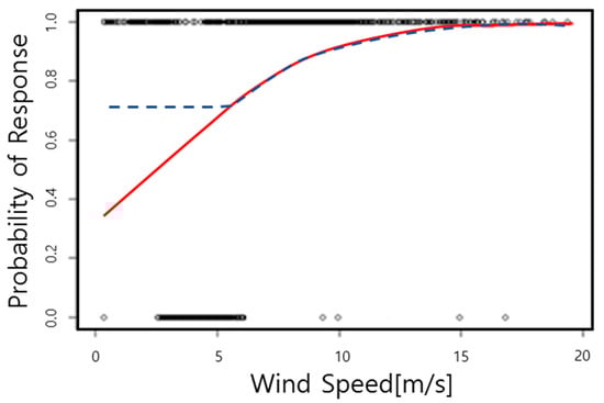
Figure A1.
The statistical model for estimating accuracy of power curves for additional turbine using logistic regression (The red line is statistical model and the blue line is fixed minimum value).
We also applied the same method to the additional turbine to perform wind forecasting on 8 January 2016. The following results were obtained.
Table A3.
The probability that outputs for additional turbine exist within a tolerance band.
Table A3.
The probability that outputs for additional turbine exist within a tolerance band.
| Wind Speed [m/s] | Accuracy [%] |
|---|---|
| 4.0 | 74.97 |
| 5.0 | 74.97 |
| 6.0 | 74.97 |
| 7.0 | 80.57 |
| 8.0 | 85.57 |
| 9.0 | 88.66 |
| 10.0 | 91.71 |
| 11.0 | 94.48 |
| 12.0 | 96.15 |
| 13.0 | 97.07 |
| 14.0 | 97.82 |
| 15.0 | 98.33 |
| 16.0 | 99.58 |
| 17.0 | 99.12 |
| 18.0 | 99.33 |
| 19.0 | 99.57 |
| 20.0 | 99.69 |
Table A4.
Measured and forecasted wind power outputs to additional turbine on 8 January 2016.
Table A4.
Measured and forecasted wind power outputs to additional turbine on 8 January 2016.
| Hour | Measured [kW] | SVR (Single Variable) [kW] | SVR (Multi Variables) [kW] |
|---|---|---|---|
| 1 | 332.540 | 311.150 | 308.801 |
| 2 | 346.513 | 335.553 | 320.253 |
| 3 | 325.885 | 323.321 | 299.133 |
| 4 | 278.277 | 265.841 | 239.944 |
| 5 | 238.735 | 217.666 | 200.565 |
| 6 | 202.201 | 200.712 | 189.074 |
| 7 | 173.578 | 171.336 | 175.348 |
| 8 | 103.105 | 106.735 | 108.191 |
| 9 | 35.696 | 27.867 | 26.605 |
| 10 | 21.520 | 25.571 | 24.042 |
| 11 | 44.146 | 64.988 | 59.111 |
| 12 | 57.347 | 66.005 | 58.541 |
| 13 | 64.183 | 70.684 | 64.431 |
| 14 | 100.914 | 95.935 | 97.406 |
| 15 | 101.308 | 98.109 | 103.570 |
| 16 | 71.782 | 84.313 | 69.181 |
| 17 | 47.644 | 58.474 | 46.167 |
| 18 | 17.291 | 26.321 | 28.347 |
| 19 | 12.912 | 13.278 | 17.640 |
| 20 | 13.503 | 31.426 | 24.212 |
| 21 | 45.669 | 43.895 | 47.083 |
| 22 | 35.911 | 28.939 | 30.082 |
| 23 | 6.901 | 20.691 | 22.567 |
| 24 | 36.306 | 32.960 | 40.109 |
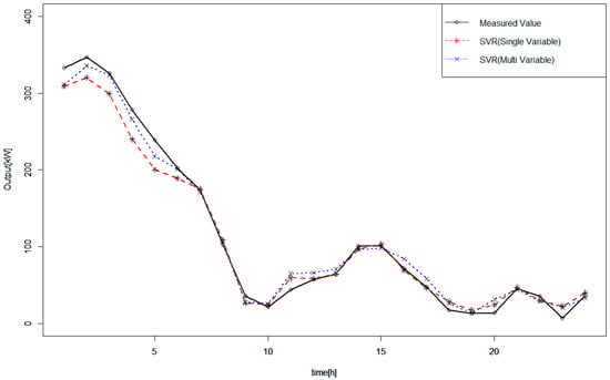
Figure A2.
Measured and forecasted wind power outputs to additional turbine on 8 January 2016.
Table A5 shows the accuracy of forecasted values.
Table A5.
Accuracy of SVR model and Persistence method (8 January 2016).
Table A5.
Accuracy of SVR model and Persistence method (8 January 2016).
| Hour | Correlation | R-Squared | RMSE |
|---|---|---|---|
| SVR (single variables) | 0.9966 | 0.9931 | 15.8013 |
| SVR (multi variables) | 0.9970 | 0.9937 | 10.7970 |
| Persistence method | 0.9656 | 0.9325 | 32.0529 |
References
- REN21. Renewable 2015 Global Status Report; Renewable Energy Policy Network for the 21th Century (REN21): Paris, France, 2015. [Google Scholar]
- IEA. World Energy Outlook 2015; International Energy Agency: Paris, France, 2015. [Google Scholar]
- O’Hair, E.; Giesselmann, M.G. Comparative analysis of regression and artificial neural network models for wind turbine power curve estimation. J. Sol. Energy Eng. 2001, 123, 327–332. [Google Scholar]
- Department of Statistics. Available online: http://www.stat.cmu.edu/~cshalizi/uADA/12/lectures/ch12.pdf (accessed on 8 June 2017).
- Chang, W.-Y. A literature review of wind forecasting methods. J. Power Energy Eng. 2014, 2, 161–168. [Google Scholar] [CrossRef]
- Foley, A.M.; Leahy, P.G.; McKegh, E.J. Wind power forecasting & prediction methods. In Proceedings of the 9th International Conference on Environment and Electrical Engineering, Prague, Czech Republic, 16–19 May 2010. [Google Scholar]
- Abdelaziz, A.Y.; Rahman, M.A.; El-Khayat, M.M.; Hakim, M.A. Short term wind power forecasting using autoregressive integrated moving average approach. J. Energy Power Eng. 2013, 7, 2089. [Google Scholar]
- Pinson, P.; Madsen, H.; Nielsen, H.A.; Papaefthymiou, G.; Klöckl, B. From probabilistic forecasts to statistical scenarios of short-term wind power production. Wind Energy 2008, 12, 51–62. [Google Scholar] [CrossRef]
- Pinson, P.; Madsen, H.; Giebel, G.; Kariniotakis, G.; von Bremen, L.; Marti, I. Forecasting of wind generation: Recent advances and future challenges. In Proceedings of the European Wind Energy Conference and Exhibition, Milan, Italy, 7–10 May 2007. [Google Scholar]
- Costa, A.; Crespo, A.; Navarro, J.; Lizcano, G.; Madsen, H.; Feitosa, E. A review on the young history of the wind power short-term prediction. Renew. Sustain. Energy Rev. 2007, 12, 1725–1744. [Google Scholar] [CrossRef]
- Choi, S.Y.; Han, K.Y.; Kim, B.H. Comparison of different multiple linear regression models for real-time flood stage forecasting. J. Korean Soc. Civ. Eng. 2012, 32, 9–20. [Google Scholar]
- Law, M. A Simple Introduction to Support Vector Machines. Available online: https://www.cise.ufl.edu/class/cis4930fa15idm/notes/intro_svm_new.pdf (accessed on 8 June 2017).
- Drucker, H.; Burges, C.J.C.; Kaufman, L.; Smola, A.; Vapnik, V. Support vector regression machines. Adv. Neural Inf. Proc. Syst. 1996, 9, 155–161. [Google Scholar]
- Hearst, M.A.; Dumais, S.T.; Osuna, E.; Platt, J.; Scholkopf, B. Support vector machines. IEEE Intell. Syst. Appl. 1998, 13, 18–28. [Google Scholar] [CrossRef]
- Press, S.J.; Wilson, S. Choosing between logistic regression and discriminant analysis. J. Am. Statist. Assoc. 1978, 73, 699–705. [Google Scholar] [CrossRef]
- Hellevik, O. Linear versus logistic regression when the dependent variable is a dichotomy. Qual. Quant. 2009, 43, 59–74. [Google Scholar] [CrossRef]
- Peduzzi, P.; Concato, J.; Kemper, E.; Holford, T.R.; Feinstein, A.R. A simulation study of the number of events per variable in logistic regression analysis. J. Clin. Epidemiol. 1996, 49, 1373–1379. [Google Scholar] [CrossRef]
- Friedman, J.; Hastie, T.; Tibshirani, R. Additive logistic regression: A statistical view of boosting (with discussion and a rejoinder by the authors). Ann. Statist. 2000, 28, 337–407. [Google Scholar] [CrossRef]
- Jordan, A. On discriminative vs. generative classifiers: A comparison of logistic regression and naive bayes. Adv. Neural Inf. Proc. Syst. 2002, 14, 841–848. [Google Scholar]
- Hayes, A.F.; Matthes, J. Computational procedures for probing interactions in OLS and logistic regression: SPSS and SAS implementations. Behav. Res. Methods 2009, 41, 924–936. [Google Scholar] [CrossRef] [PubMed]
- Burges, C.J.C. A tutorial on support vector machines for pattern recognition. Data Min. Knowl. Discov. 1998, 2, 121–167. [Google Scholar] [CrossRef]
- Du, Y.; Lu, J.; Li, Q.; Deng, Y.L. Short-term wind speed forecasting of wind farm based on least square-support vector machine. Power Syst. Technol. 2008, 32, 62–66. [Google Scholar]
- Lei, M.; Shiyan, L.; Jiang, C.; Liu, H.; Zhang, Y. A review on the forecasting of wind speed and generated power. Renew. Sustain. Energy Rev. 2009, 13, 915–920. [Google Scholar] [CrossRef]
- Zhu, L. Support Vector Machines. Available online: http://www.pstat.ucsb.edu/student%20seminar%20doc/Kernel%20SVM.pdf (accessed on 8 June 2017).
- Liu, Y.; Shi, J.; Yang, Y.; Lee, W.-J. Short-term wind-power prediction based on wavelet transform—Support vector machine and statistic-characteristics analysis. IEEE Trans. Ind. Appl. 2012, 48, 1136–1141. [Google Scholar] [CrossRef]
- Meyer, D. Support Vector Machines. Available online: http://dictionnaire.sensagent.leparisien.fr/SUPPORT%20VECTOR%20MACHINE/en-en/ (accessed on 8 June 2017).
- Meyer, D.; Technikum Wien, F.H. Support Vector Machines—The Interface to Libsvm in Package e1071. Available online: https://cran.r-project.org/web/packages/e1071/vignettes/svmdoc.pdf (accessed on 8 June 2017).
- Support Vector Regression in R. Available online: http://www.svm-tutorial.com/2014/10/support-vector-regression-r/ (accessed on 8 June 2017).
© 2017 by the authors. Licensee MDPI, Basel, Switzerland. This article is an open access article distributed under the terms and conditions of the Creative Commons Attribution (CC BY) license (http://creativecommons.org/licenses/by/4.0/).