Volatility Modelling of the JSE Top40 Index: Assessing the GAS Framework Against GARCH and Hybrid GARCH–XGBoost

Abstract

This paper studies the volatility dynamics of the JSE Top40 Index by estimating a univariate GAS model with time-varying location, scale, and shape parameters (identity score scaling) and comparing its density and point-forecast performance against a stand-alone ARMA(3,2)–EGARCH(1,1) model and a hybrid ARMA(3,2)–EGARCH(1,1)–XGBoost framework. The GAS model is estimated on 3515 daily observations, and several conditional densities are examined. The Student-t GAS model (GAS–STD) obtains the lowest information criteria within the GAS family (AIC = 10,188.142; BIC = 10,243.626) and exhibits statistically significant persistence in location and scale dynamics. Statistical diagnostics provide evidence of correct density calibration (normalised log score = 1.1932; Uniform score = 0.4417), although residual skewness remains (IID-Test skewness $p=0.0134$). Out-of-sample analysis shows that GAS–STD performs strongly in density and risk forecasting, producing accurate 5% VaR and ES paths and passing coverage backtests (Kupiec LRuc $p=0.8414$; DQ $p=0.2281$). However, short-horizon point forecasts are most accurately produced by the Hybrid ARMA(3,2)–EGARCH(1,1)–XGBoost model (RMSE = 0.1386). The full Diebold-Mariano (DM) test confirms that all pairwise differences in predictive accuracy are statistically significant, and the model confidence set (MCS) procedure identifies the Hybrid model as the sole superior model at the 5% significance level, indicating that both ARMA(3,2)–EGARCH(1,1) and GAS–STD are statistically inferior. Simulation experiments illustrate that the tail behaviour of the Student-t distribution is sensitive to the degrees-of-freedom parameter $\nu$. For example, a Student-t distribution with $\nu =5$ exhibits total kurtosis of approximately $7.32$, indicating heavier tails compared to the Gaussian distribution. Overall, GAS–STD is a strong density and risk model for the JSE Top40, while the hybrid framework excels in short-term volatility forecasting.

1. Introduction

Volatility modelling has been the focus in financial econometrics due to its importance for asset pricing, portfolio decisions, and financial stability. Financial series tend to exhibit stylised features such as volatility clustering, fat tails, and asymmetric shocks (Bollerslev, 1986; Engle, 1982; Nelson, 1991). Historical models such as autoregressive conditional heteroscedasticity (ARCH) and generalised autoregressive conditional heteroscedasticity (GARCH) have been highly useful, but their restrictive assumptions prevent them from fully capturing the richness of return distributions. Developments such as exponential GARCH (EGARCH) by Nelson (1991) and Glosten, Jagannathan, and Runkle GARCH (GJR–GARCH) by Glosten et al. (1993) addressed asymmetries more effectively, and even multivariate GARCH forms have been introduced (Bauwens et al., 2006). Emerging markets are generally characterised by higher volatility because of greater exposure to macroeconomic disturbances, institutional uncertainties, and fluctuations in global capital flows. The Johannesburg Stock Exchange (JSE), being the largest stock market in Africa, offers an important setting for examining such dynamics. In particular, the JSE Top40 Index reflects the most liquid and capitalised businesses and, hence, serves as a benchmark for local and foreign investors (Jefferis & Smith, 2005). Modelling its volatility is therefore crucial for policy, risk management, and investment. Recent developments in machine learning have delivered alternatives to conventional econometric approaches. eXtreme Gradient Boosting (XGBoost) (Chen & Guestrin, 2016) is a robust gradient boosting method that has become very popular, and combination models of GARCH with XGBoost have been shown to improve the accuracy of short-term predictions (Maingo et al., 2025a). Furthermore, ARIMA-ANN hybrid models remain widely used in financial contexts, as demonstrated by the hybrid model for GDP forecasting in Nepal (Chaudhary & Uprety, 2024), while CEEMDAN–based hybrid models integrated with machine learning and optimization algorithms such as MARS and PSO continue to gain prominence in time series prediction (Garai et al., 2024). However, these hybrids often lack interpretability, limiting their utility in regulatory applications. Creal et al. (2013) proposed a promising alternative with the generalised autoregressive score (GAS) model, which was later extended by A. C. Harvey (2013). GAS models learn parameters by iterating through the score of the conditional likelihood, making them highly sensitive to fresh data.

Recent advancements in volatility modelling have increasingly employed hybrid and machine learning techniques to better capture nonlinear patterns and shifts in market regimes. Examples of such approaches include regime-switching Markov Switching–GARCH (MS–GARCH) integrated with neural networks (NN), Support Vector Regression–GARCH (SVR–GARCH), and Neural Networks–GARCH (NN–GARCH), which have been shown to improve short-term forecasting accuracy (Bildirici & Ersin, 2016; Sun & Yu, 2020; Zhao et al., 2024). Moreover, mixed data sampling (MIDAS) models that incorporate fundamental variables at different frequencies allow researchers to combine macroeconomic and financial information with daily return data, thereby enhancing predictive performance (Eniayewu et al., 2024; Fang et al., 2020). Although this study primarily concentrates on the GAS framework and hybrid ARMA–EGARCH–XGBoost models, these alternative methods provide valuable complementary insights and represent promising directions for future research.

Empirical evidence indicates that the GAS models outperform conventional GARCH in density forecasting and risk measurement, particularly under heavy-tailed or asymmetric distributions (Lazar & Xue, 2020). Building on these theoretical results, Ardia et al. (2019) built the R package (version $4.4.0$) GAS that provides practical implementation tools and demonstrated its application using examples to financial asset returns, confirming the ability of the framework to model time-varying conditional densities. Implementations in African markets augment this affirmation further. For instance, Babatunde et al. (2021) compared GARCH and GAS models in the forecasting of daily stock prices on the Nigerian Stock Exchange and found that GAS under the Student-t as well as skewed Student-t distributions outperformed GARCH in volatility forecasting but that EGARCH was good under certain distributional assumptions. In parallel, Yaya et al. (2016) analysed the Nigerian All Share Index and showed that GAS-type models, including Beta-t–EGARCH, provided a superior explanation of jumps, outliers, and asymmetry relative to traditional GARCH models. Collectively, these papers show that GAS-based models provide better density forecasts and tail risk estimation than traditional GARCH, but their application to emerging markets remains relatively rare, and comparison studies with hybrid econometric and machine learning models remain scarce.

The study gap motivating the present work is that while volatility modelling in South Africa has been heavily studied by using GARCH-type models (Maingo et al., 2025b; Venter & Mare, 2020), the generalised autoregressive score (GAS) framework has received little attention, and very few studies have comparatively assessed its performance with hybrid econometric-machine learning methodologies such as GARCH–XGBoost. To address this gap, the present study employs the GAS framework to estimate and forecast the volatility of the JSE Top40 Index and compares its result with GARCH and ARMA–EGARCH–XGBoost models. The article makes four significant contributions to the literature. First, it offers one of the first comprehensive uses of GAS in South African equity markets, thereby extending its use to an important emerging market. Second, it undertakes systematic benchmarking of GAS with respect to both standard econometric and hybrid machine learning approaches, yielding comparative results into the relative performance of the latter two. Third, it shows that GAS is superior in density calibration and tail risk prediction, whereas hybrid models exhibit superior performance in short-horizon point prediction. Finally, through simulation tests, the paper emphasises the central role played by heavy-tailed distributions in modelling South African equities’ extreme return dynamics. In total, these contributions enrich volatility modelling literature and provide recommendations for practitioners, such as investors, regulators, and policymakers, who wish to pursue risk management in the emerging market setting.

2. Data and Methodology

2.1. Data

The study is going to use daily closing prices of the JSE Top40 Index for a specific time period from 31 January 2011 to 25 February 2025, totalling 3515 trading days. The data, which are freely available, can be accessed at https://za.investing.com/indices/ftse-jse-top-40-historical-data (accessed on 25 April 2025). The data are collected over a five-day trading week. To enhance the robustness and comparative strength of the analysis, an extended dataset covering the period from 3 January 2011 to 27 October 2025, totalling 3704 trading days, was also used for comparison. The JSE Top 40 Index data were compared with the MOEX Russian Index over the same period. The daily MOEX Russian Index data were obtained from the Investing.com database, accessible at https://in.investing.com/indices/mcx-historical-data (accessed on 4 November 2025). Both datasets consist of daily observations and are used to provide broader market coverage and assess the robustness of the proposed method under different market conditions. For forecast evaluation, the in-sample (estimation) period covers 31 January 2011 to 29 February 2024, while the out-of-sample (forecast) period spans 1 March 2024 to 25 February 2025. The rolling window forecasting procedure and 1-day-ahead forecast methodology are described in detail in Section 3.2.3.

2.2. Methodology

The modelling framework proposed in this study is given in the flow chart in Figure 1.

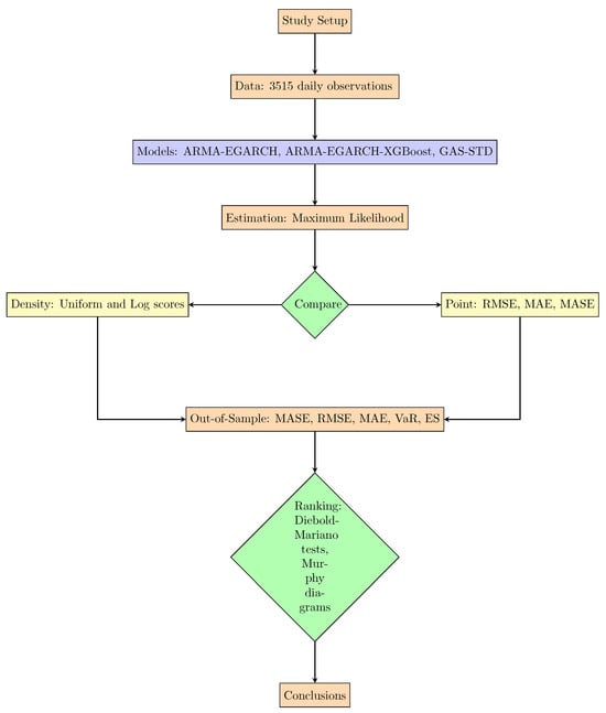
Figure 1. Stepwise work flow diagram of the modelling framework.

2.2.1. The GAS Models

The GAS model is a flexible class of time series models that extends the traditional GARCH framework by offering a more adaptive and dynamic manner to model time-varying volatility. This model was introduced by A. C. Harvey (2013) and Creal et al. (2013) and leverages the score of the conditional likelihood function, which measures how sensitive the likelihood is to implement changes in the model parameters. By utilising the score, the GAS model updates volatility at each time point, enabling it to respond more flexibly to new information and adjust volatility estimates accordingly. A major benefit of the GAS model is its robustness to outliers, as the score functions minimise the impact of extreme values by reducing the weight of isolated observations (Alanya-Beltran, 2022; A. C. Harvey, 2013; Junior & Alagidede, 2020). This leads to it being well-suited for modelling financial time series data, which often exhibit fat tails and skewness (A. C. Harvey, 2013; Opschoor et al., 2018). Moreover, the GAS process permits for the inclusion of additional time series features, such as asymmetry and long memory effects, making it highly versatile in capturing complex dynamics in financial markets. Furthermore, the model can be estimated efficiently using maximum likelihood estimation (MLE), making it straightforward to implement (Ardia et al., 2019). This flexibility, combined with its robustness and ability to handle complicated features of financial data, makes the GAS model a powerful tool for capturing volatility persistence and modelling time-varying volatility in financial time series.

2.2.2. GAS Models Specification

Let $y_t$ be a $N\times 1$ vector representing the dependent variable of interest at time t. The time-varying parameter vector is denoted by ${\lambda }_t$, while $x_t$ represents a set of exogenous variables (also called covariates), influencing the system. Moreover, $\varphi$ is a vector of static parameters that remain constant over time. Define $X^t=\{x_1,\dots ,x_n\}$, ${\Lambda }^t=\{{\lambda }_1,\dots ,{\lambda }_t\}$, and $Y^t=\{y_1,\dots ,y_t\}$. At any given time t, the available information consists of $\{{\lambda }_t,{\mathrm{F}}_t\}$, where ${\mathrm{F}}_t$ is defined as

$$\begin{array}{c}\hfill {\mathrm{F}}_t=\{Y^{t-1},{\Lambda }^{t-1},X^t\},\mathrm{for}t=1,\dots ,n.\end{array}$$

(1)

It is assumed that the dependent variable $y_t$ is generated from an observation density function given by

$$\begin{array}{c}\hfill y_t\sim p\left(y_t\right|{\lambda }_t,{\mathrm{F}}_t;\varphi ).\end{array}$$

(2)

Additionally, we assume that the process for updating the time-varying parameter ${\lambda }_t$ follows a standard autoregressive update equation, specifically given by

$$\begin{array}{c}\hfill {\lambda }_{t+1}=\alpha +\sum _{i=1}^p{A}_i{s}_{t-i+1}+\sum _{j=1}^q{B}_j{\lambda }_{t-j+1},\end{array}$$

(3)

where $\alpha$ is a vector of constants, the coefficient matrices $A_i$ and $B_j$ have dimensions that are suitable for $i=1,\dots ,p$ and $j=1,\dots ,q$, respectively. Additionally, $s_t$ is a function of past data, defined as $s_t=s_t(y_t,{\lambda }_t,{\mathrm{F}}_t;\varphi )$. The unknown coefficients in Equation (3) are functions of the parameter vector $\varphi$; specifically, $\alpha =\alpha \left(\varphi \right)$, $A_i=A_i\left(\varphi \right)$, and $B_j=B_j\left(\varphi \right)$ for $i=1,\dots ,p$ and $j=1,\dots ,q$. The method utilised by the GAS model is based on the observation density (2) for a given parameter ${\lambda }_t$. When an observation $y_t$ occurs, we update the time-varying parameter ${\lambda }_t$ to the next period, $t+1$ using Equation (3) with

$$\begin{array}{c}\hfill s_t=S_t·{\nabla }_t,{\nabla }_t={\displaystyle \frac{\partial lnp\left(y_t\right|{\lambda }_t,{\mathrm{F}}_t;\varphi )}{\partial {\lambda }_t}},S_t=S(t,{\lambda }_t,{\mathrm{F}}_t;\varphi ).\end{array}$$

(4)

Here, $S(·)$ represents a matrix function. Since the updating mechanism in Equation (3) depends on the scaled score vector in Equation (4), we define Equations (2)–(5) as the foundation of the GAS model with orders p and q. For simplicity, we refer to this model as GAS$(p,q)$. The use of the score to update ${\lambda }_t$ is straightforward. The steepest climb route improves the model’s local fit in terms of likelihood or density at time t, based on the current position of parameter ${\lambda }_t$. This indicates the obvious direction for updating the parameter. The score is based on the whole density, not just the first- or second-order moments of the observations $y_t$. The GAS framework stands out among observation-driven techniques in the literature. The GAS model uses the whole density structure to transform data and update time-varying parameters ${\lambda }_t$. The GAS model’s scaling matrix $S_t$ provides flexibility in how the score is updated for ${\lambda }_t$. Changing the scaling matrix $S_t$ yields a unique GAS model. Each of these models has unique statistical and empirical aspects that need to be examined separately. Scaling based on score variance is a common approach in several scenarios. For instance, we can provide the scaling matrix as

$$\begin{array}{c}\hfill S_t={\mathfrak{I}}_{t|t-1}^{-\gamma },{\mathfrak{I}}_{t|t-1}={\mathrm{E}}_{t-1}\left[{\nabla }_t{\nabla }_t^{\prime }\right],\end{array}$$

(5)

where the expectation ${\mathrm{E}}_{t-1}$ is computed based on the conditional distribution of $y_t|y_{1:t-1}$. The parameter $\gamma$ typically takes values of $0,{\displaystyle \frac{1}{2}},\mathrm{or}1$, though other choices for $S_t$ values are also feasible. When $\gamma =0$, $S_t$ becomes the identity matrix $\left(I\right)$, implying no scaling. If $\gamma ={\displaystyle \frac{1}{2}}$, the conditional score ${\nabla }_t$ is multiplied by the square root of its covariance matrix ${\mathfrak{I}}_t$, whereas for $\gamma =1$, it is instead multiplied by the inverse of its covariance matrix ${\mathfrak{I}}_t$. The scaled score $s_t$ follows a martingale difference property concerning the distribution of $y_t|y_{1:t-1}$, ensuring that ${\mathrm{E}}_{t-1}\left[s_t\right]=0$ for every t. From an economic perspective, the GAS model updates its parameters based on new market information. When the score is large, typically during periods of elevated volatility or market shocks, the model increases its volatility estimates. Conversely, small score values correspond to stable market conditions. Therefore, the GAS mechanism effectively captures investors’ adaptive responses and changes in market regimes, dynamically adjusting the conditional volatility according to observed returns.

2.2.3. GARCH Models

For comparative analysis, two additional models are considered: the conventional (generalised autoregressive heteroscedasticity) GARCH and the exponential GARCH (EGARCH) models, which serve as volatility benchmarks against the proposed GAS framework.

GARCH(1,1) Model

The GARCH(1,1) model, introduced by Bollerslev (1986), models conditional heteroscedasticity by allowing the conditional variance to depend on past squared shocks and its own lagged values:

$$r_t=\mu +{\epsilon }_t,{\epsilon }_t={\sigma }_t{z}_t,z_t\sim N(0,1),$$

(6)

$${\sigma }_t^2=\omega +\alpha {\epsilon }_{t-1}^2+\beta {\sigma }_{t-1}^2,$$

(7)

where $\omega >0$, $\alpha ,\beta \ge 0$, and $\alpha +\beta <1$ ensures covariance stationarity. The model effectively captures volatility clustering (where periods of high volatility are followed by calm periods), which is a common stylised fact observed in financial time series (Engle, 1982).

EGARCH(1,1) Model

To accommodate asymmetries in volatility response to positive and negative shocks,  (Nelson, 1991) proposed the EGARCH(1,1) model, expressed as

$$log\left({\sigma }_t^2\right)=\omega +\beta log\left({\sigma }_{t-1}^2\right)+\alpha \left({\displaystyle \frac{|{\epsilon }_{t-1}|}{{\sigma }_{t-1}}}-\sqrt{{\displaystyle \frac{2}{\pi }}}\right)+\gamma {\displaystyle \frac{{\epsilon }_{t-1}}{{\sigma }_{t-1}}}.$$

(8)

The logarithmic specification guarantees positive variance without parameter constraints, while the parameter $\gamma$ captures leverage effects (asymmetric reactions) of volatility to positive and negative shocks.

2.2.4. XGBoost Model

The eXtreme Gradient Boosting (XGBoost) algorithm, developed by Chen and Guestrin (2016), is an ensemble learning technique based on gradient boosting decision trees. It builds a sequence of trees where each subsequent tree corrects the errors of the previous ones. The model minimises an objective function composed of a loss term and a regularisation term:

$$\mathcal{L}\left(\varphi \right)=\sum _{i=1}^{n}l(y_i,{\widehat{y}}_i)+\sum _{k=1}^K\Omega \left(f_k\right),$$

(9)

where $l(y_i,{\widehat{y}}_i)$ is a differentiable convex loss function measuring the difference between the observed and predicted values, and $\Omega \left(f_k\right)$ is a regularisation term controlling model complexity:

$$\Omega \left(f_k\right)=\gamma T+{\displaystyle \frac{1}{2}}\lambda {\parallel w\parallel }^2,$$

(10)

with T denoting the number of leaves in the k-th tree and w the leaf weights.

XGBoost enhances predictive accuracy by combining multiple weak learners to form a strong ensemble model. Its main advantage lies in its ability to capture nonlinear relationships and higher-order interactions that traditional econometric models often fail to detect. Moreover, it effectively prevents overfitting through L1/L2 regularisation and shrinkage, while maintaining computational efficiency and scalability for large, high-dimensional datasets. These features make XGBoost particularly suitable for short-term financial prediction and volatility forecasting tasks (Nadarajah et al., 2025).

2.2.5. GARCH–XGBoost Hybrid Model

The volatility of the JSE Top40 index is modelled using a hybrid GARCH–XGBoost approach, following steps similar to the frameworks proposed by Maingo et al. (2025a). The process begins with extraction and preprocessing of historical JSE Top40 index data. Log-returns are computed as $r_t=100\times (ln\left(Z_t\right)-ln\left(Z_{t-1}\right))$, transforming price levels into a stationary series suitable for volatility modelling. A GARCH-type model is then fitted to the log-returns to capture conditional heteroscedasticity and produce standardised residuals. Lag-based features are constructed from these residuals and used as inputs for the XGBoost model. The data are split into training and test sets, and the XGBoost model is trained to capture nonlinear patterns and improve volatility forecasts. Finally, the trained model is used to forecast future volatility, and performance is evaluated using appropriate metrics.

In this study, hyperparameter tuning and feature construction for the XGBoost model are performed systematically. Lagged and rolling features are created from the standardised residuals obtained from the fitted ARMA(3,2)-EGARCH(1,1) model. Specifically, 15 lagged residuals and rolling statistics over windows of 2, 3, 5, 10, and 20 periods (mean and standard deviation) are constructed as input features. The dataset is split into training (60%), calibration (20%), and test sets (20%) to ensure robust evaluation. XGBoost training is performed with 5-fold cross-validation and early stopping (20 rounds) to identify the optimal number of boosting iterations. Key hyperparameters are set as follows: learning rate $\eta =0.05$, maximum tree depth = 4, subsample = 0.8, and column subsample = 0.8. Predictions on the test set are obtained using the final model trained on the training data, and prediction intervals are constructed based on residual quantiles from the calibration set. This procedure ensures that the hybrid model effectively captures nonlinear patterns in volatility and provides accurate and well-calibrated forecasts.

The proposed Hybrid ARMA(3,2)–EGARCH(1,1)–XGBoost volatility forecasting framework is summarised in Algorithm 1. The hyperparameter configuration for the XGBoost component is provided in Table 1.

• XGBoost Pseudocode and Hyperparameter Table.

Table 1. Hyperparameter configuration for XGBoost component of the hybrid model.

Parameter	Value/Description
Objective function	reg:squarederror
Learning rate ($\eta$)	0.05
Maximum tree depth	4
Subsample ratio	0.8
Column subsample ratio	0.8
Number of boosting rounds	Determined via 5-fold CV with early stopping (20 rounds)
Cross-validation folds	5
Early stopping rounds	20
Random seed	548

Table 1. Hyperparameter configuration for XGBoost component of the hybrid model.

Parameter	Value/Description
Objective function	reg:squarederror
Learning rate ($\eta$)	0.05
Maximum tree depth	4
Subsample ratio	0.8
Column subsample ratio	0.8
Number of boosting rounds	Determined via 5-fold CV with early stopping (20 rounds)
Cross-validation folds	5
Early stopping rounds	20
Random seed	548

Algorithm 1 Hybrid ARMA(3,2)–EGARCH(1,1)–XGBoost Volatility Forecasting Framework

1: Input: Historical JSE Top40 index prices ${\left\{Z_t\right\}}_{t=1}^T$ 2: Compute log-returns: $r_t=100\times (ln{Z}_t-ln{Z}_{t-1})$ 3: Fit ARMA(3,2)–EGARCH(1,1) model to $r_t$ to obtain standardised residuals $z_t$ 4: Construct lag-based and rolling statistical features from $\left\{z_t\right\}$: Lags: $z_{t-1},z_{t-2},\dots ,z_{t-15}$ Rolling means and standard deviations over windows $k=\{2,3,5,10,20\}$ 5: Split data into training (60%), calibration (20%), and test (20%) sets 6: Perform 5-fold cross-validation with early stopping (20 rounds) to tune the optimal number of boosting iterations 7: Train XGBoost model using training set with selected hyperparameters 8: Predict standardised residuals on calibration and test sets 9: Output: Predicted conditional volatility series

2.2.6. Parameter Estimation

After specifying the conditional distribution $p\left(y_t\right|{\lambda }_t,{\mathrm{F}}_t;\varphi )$, the following step is to estimate the model parameters $\varphi$. A common method is maximum likelihood estimation (MLE). We aim to find $\varphi$ that maximises the log-likelihood ($\mathrm{LL}$) function given the observed data $Y^t=\{y_1,\dots ,y_t\}$:

$$\begin{array}{c}\hfill \mathcal{L}\left(\varphi \right)=\sum _{k=1}^{t}logp\left(y_t\right|{\lambda }_t,{\mathrm{F}}_t;\varphi )\end{array}$$

(11)

In several GAS and GARCH-type models, ${\lambda }_t$ is dynamically updated, and hence, the likelihood is conditionally examined at each step using past information. Under practical conditions, numerical optimisation techniques are employed to solve the following Equation (12):

$$\begin{array}{c}\hfill \widehat{\varphi }=arg\underset{\varphi }{max}\mathcal{L}\left(\varphi \right),\end{array}$$

(12)

where $\mathcal{L}\left(\varphi \right)={\sum }_{k=1}^t\log p\left(y_t\right|{\lambda }_t,{\mathrm{F}}_t;\varphi )$ is the log-likelihood function as shown in Equation (11).

2.2.7. Evaluation Metrics

To assess the performance of models, we use evaluation metrics such as Akaike information criterion ($\mathrm{AIC}$), and Bayesian information criterion. The R software package is used to compute the value of $\mathrm{AIC}$, and $\mathrm{BIC}$. The formulas for $\mathrm{AIC}$ and $\mathrm{BIC}$ are given by the following Equation (13):

$$\begin{array}{c}\hfill \mathrm{AIC}=-2\mathcal{L}\left(\widehat{\varphi }\right)+2k,\mathrm{and}\mathrm{BIC}=-2\mathcal{L}\left(\widehat{\varphi }\right)+klog\left(n\right),\end{array}$$

(13)

where $\mathcal{L}\left(\widehat{\varphi }\right)$ denotes the maximised log-likelihood, k represents the number of estimated parameters in the model, and n is the sample size. The model with the lowest value of $\mathrm{AIC}$ and $\mathrm{BIC}$ is considered.

2.2.8. Forecast Accuracy Measures

To evaluate how well the prediction model performs, this study employs several accuracy metrics, including the mean absolute square error (MASE), mean absolute error (MAE), and root mean square error (RMSE). The corresponding formulas are presented in Equations (14)–(16).

$$\begin{array}{c}\hfill \mathrm{MASE}={\displaystyle \frac{\frac{1}{n}{\sum }_{t=1}^n|y_t-{\widehat{y}}_t|}{\frac{1}{n-1}{\sum }_{t=2}^n|y_t-y_{t-1}|}}\end{array}$$

(14)

$$\begin{array}{c}\hfill \mathrm{MAE}={\displaystyle \frac{1}{n}}\sum _{t=1}^n|y_t-{\widehat{y}}_t|\end{array}$$

(15)

$$\begin{array}{c}\hfill \mathrm{RMSE}=\sqrt{{\displaystyle \frac{1}{n}}\sum _{t=1}^n{(y_t-{\widehat{y}}_t)}^2}\end{array}$$

(16)

2.2.9. Statistical Test of Predictive Accuracy

To statistically evaluate the difference in the accuracy of the two rival models’ forecasts, this study applies the Diebold–Mariano (DM) test of Diebold and Mariano (1995). The DM test offers a statistical test for ascertaining if the difference between the accuracy of the two models is statistically significant by analysing the series of loss differentials between their forecast errors. Since the competing models in this study are non-nested, the DM test is theoretically appropriate for assessing differences in predictive performance.

Let $e_{1,t}$ and $e_{2,t}$ represent the forecast errors from models 1 and 2 at time t. Given a chosen loss function $L(·)$, such as the squared error loss $L\left(e_{j,t}\right)=e_{j,t}^2$ or absolute error loss $L\left(e_{j,t}\right)=\left|e_{j,t}\right|$, the loss differential is given as

$$d_t=L\left(e_{1,t}\right)-L\left(e_{2,t}\right),t=1,2,\dots ,T$$

(17)

The null and alternative hypotheses $(H_0\&H_1)$ of the DM test are

$$H_0:\mathbb{E}\left[d_t\right]=0(\mathrm{equal}\mathrm{predictive}\mathrm{accuracy})$$

(18)

$$H_1:\mathbb{E}\left[d_t\right]\ne 0(\mathrm{different}\mathrm{predictive}\mathrm{accuracy})$$

(19)

The sample mean of the loss differential is determined using the following mathematical formula:

$$\overline{d}={\displaystyle \frac{1}{T}}\sum _{t=1}^T{d}_t$$

(20)

Since forecast horizons longer than one period ($h>1$) may induce autocorrelation in $d_t$, the long-run variance of the loss differential must be estimated. This is fulfilled using a heteroscedasticity and autocorrelation consistent (HAC) estimator, given by

$${\widehat{\sigma }}_d^2={\widehat{\gamma }}_d\left(0\right)+2\sum _{k=1}^{h-1}{\widehat{\gamma }}_d\left(k\right),$$

(21)

where ${\widehat{\gamma }}_d\left(k\right)$ denotes the sample autocovariance of $d_t$ at lag k.

The DM statistic is then given by

$$DM={\displaystyle \frac{\overline{d}}{\sqrt{{\widehat{\sigma }}_d^2/T}}}$$

(22)

Assuming the null hypothesis $\left(H_0\right)$ and in conjunction with proper regularity conditions, the DM statistic is asymptotically standard normal, $DM\sim N(0,1)$. A two-sided test rejects $H_0$ if $\left|DM\right|>z_{\alpha /2}$, where $z_{\alpha /2}$ is the standard normal critical value. However, the asymptotic approximation can be deceptive in finite samples, particularly for small T or large forecast horizons. To address this, D. Harvey et al. (1997) proposed a small-sample correction, which is referred to as the HLN correction. The correction scales the DM statistic down and ties it to a Student’s t-distribution with $T-1$ degrees of freedom, thereby reducing size distortions. Through this process, the DM test allows us to ascertain whether a model’s one-step-ahead forecasting performance differs significantly from that of its competitor, offering a firm statistical basis for model comparison.

2.2.10. Value-at-Risk and Expected Shortfall

Let L denote the loss random variable (so larger L is worse). Let $F_L\left(x\right)=\mathbb{P}(L\le x)$ be its cumulative distribution function (CDF). Denote the lower $\alpha$-quantile as

$$q_{\alpha }\left(L\right)=inf\{x\in \mathbb{R}:F_L\left(x\right)\ge \alpha \}.$$

(23)

If $F_L$ is continuous and strictly increasing, then $q_{\alpha }\left(L\right)=F_L^{-1}\left(\alpha \right)$ (Acerbi & Tasche, 2002; McNeil et al., 2005).

Value-at-Risk (VaR)

The value-at-risk at level $\alpha \in (0,1)$ is defined as the $\alpha$-quantile of the loss distribution:

$${\mathrm{VaR}}_{\alpha }\left(L\right)=q_{\alpha }\left(L\right)=inf\{x\in \mathbb{R}:F_L\left(x\right)\ge \alpha \}.$$

(24)

(Standard definition by (Artzner et al., 1999; McNeil et al., 2005)).

For a normal example: If $L\sim \mathcal{N}(\mu ,{\sigma }^2)$, then

$${\mathrm{VaR}}_{\alpha }\left(L\right)=\mu +\sigma z_{\alpha },z_{\alpha }:={\Phi }^{-1}\left(\alpha \right),$$

(25)

where $\Phi$ is the standard normal CDF.

Expected Shortfall (ES)–Continuous Case

Expected shortfall at level $\alpha$ is the conditional expectation:

$${\mathrm{ES}}_{\alpha }\left(L\right)=\mathbb{E}\left[L\mid L\ge {\mathrm{VaR}}_{\alpha }\left(L\right)\right].$$

(26)

For continuous distributions (with density $f_L$),

$${\mathrm{ES}}_{\alpha }\left(L\right)={\displaystyle \frac{1}{1-\alpha }}{\int }_{{\mathrm{VaR}}_{\alpha }\left(L\right)}^{\infty }x{f}_L\left(x\right)dx.$$

(27)

If we change a variable $u=F_L\left(x\right)$ in (27), then $du=f_L\left(x\right)dx$ and $x=F_L^{-1}\left(u\right)={\mathrm{VaR}}_u\left(L\right)$.

Thus,

$${\mathrm{ES}}_{\alpha }\left(L\right)={\displaystyle \frac{1}{1-\alpha }}{\int }_{\alpha }^1{\mathrm{VaR}}_u\left(L\right)du.$$

(28)

For normal case closed form: If $L\sim \mathcal{N}(\mu ,{\sigma }^2)$, then

$${\mathrm{ES}}_{\alpha }\left(L\right)=\mu +\sigma {\displaystyle \frac{\phi \left(z_{\alpha }\right)}{1-\alpha }},$$

(29)

where $\phi$ is the standard normal PDF.

General Distributions (Robust Definition)

For possibly discontinuous distributions, a robust definition is

$${\mathrm{ES}}_{\alpha }\left(L\right)={\displaystyle \frac{1}{1-\alpha }}{\int }_{\alpha }^1{q}_u\left(L\right)du,q_u\left(L\right)=inf\{x:F_L\left(x\right)\ge u\}.$$

(30)

Coherence (Subadditivity of ES)

For any losses $L_1,L_2$ with sum $L=L_1+L_2$,

$${\mathrm{ES}}_{\alpha }\left(L\right)\le {\mathrm{ES}}_{\alpha }\left(L_1\right)+{\mathrm{ES}}_{\alpha }\left(L_2\right),$$

(31)

showing ES is subadditive (coherent) (Acerbi & Tasche, 2002; Artzner et al., 1999). In contrast, VaR need not be

$${\mathrm{VaR}}_{\alpha }(L_1+L_2)>{\mathrm{VaR}}_{\alpha }\left(L_1\right)+{\mathrm{VaR}}_{\alpha }\left(L_2\right)(\mathrm{possible}\mathrm{counterexamples}).$$

(32)

Rockafellar–Uryasev CVaR Representation

Define

$${\varphi }_{\alpha }\left(x\right):=x+{\displaystyle \frac{1}{1-\alpha }}\mathbb{E}\left[{(L-x)}_{+}\right],{\left(y\right)}_{+}:=max\{y,0\}.$$

(33)

Then,

$${\mathrm{ES}}_{\alpha }\left(L\right)=\underset{x\in \mathbb{R}}{min}{\varphi }_{\alpha }\left(x\right),$$

(34)

and any minimizer $x^{*}$ is a VaR at level $\alpha$ (Rockafellar & Uryasev, 2000).

3. Empirical Results and Discussion

3.1. Exploratory Data Analysis (EDA)

Table 2 presents the summary statistics of the log-returns series. The mean return is close to zero (0.030), indicating no persistent upward or downward drift in the series. The distribution exhibits mild negative skewness (−0.267), implying slightly more frequent negative returns than positive ones. The high kurtosis value (6.328) suggests the presence of heavy tails and potential extreme observations compared to the normal distribution. The wide range between the minimum (–10.450) and maximum (9.057) values, along with a standard deviation of 1.141, further reflects substantial volatility and variability in daily log-returns.

Table 2. Summary statistics of the log-returns.

Min	$\mathbf{Q}1$	$\mathbf{Q}2$	Mean	$\mathbf{Q}3$	Max	SD	Skew	Kurt
$-10.450$	$-0.570$	$0.052$	$0.030$	$0.668$	$9.057$	$1.141$	$-0.267$	$6.328$

Panel (a) of Figure 2 shows the JSE Top40 Index with a general increasing trend from 2011 to 2025 and steep drops during periods of distress in the market, notably around 2020, which is likely to coincide with the COVID-19 pandemic. The general increasing trend implies that the original series is not stationary because its mean and variance change over time. However, after applying the first difference to obtain the log returns on a day-to-day basis, shown in panel (b), the series turns out to be stationary with no significant long-run trend or constant mean, wandering around it. Volatility clustering also occurs in the log-return series, with episodes of high and low volatility alternating (a natural characteristic of a financial series). The probability density of log returns is graphed in panel (c) and is found to be sharply peaked with heavy tails, evidence of leptokurtic behaviour. Finally, panel (d) is the Q-Q plot, where the deviation of the tails from the straight line provides evidence of deviation from normality due to extreme observations for returns.

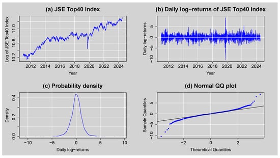
Figure 2. (a) JSE Top40 Index plot, (b) daily log-returns for JSE Top40 Index, (c) density plot of daily log-returns, and (d) normal Q-Q plot of daily log-returns.

The STL decomposition of the JSE Top 40 log-returns in Figure 3 shows that the data component fluctuates around a stable mean, confirming that the series is stationary. The seasonal component has minimal cyclical influence, suggesting weak or no seasonality. The trend component displays only slight upward and downward shifts, reflecting modest long-term volatility movements. The remainder component captures sharp spikes, such as those observed around 2020, which represent periods of market turbulence. Overall, the decomposition reveals a stationary return series characterized by volatility clustering and occasional spikes linked to market crises.

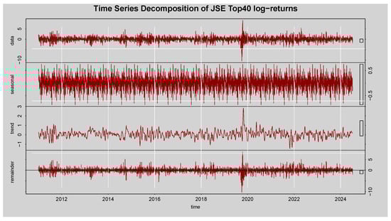
Figure 3. Decomposition of time series for the log-returns of the JSE Top40 Index.

The results of the stationarity and normality checks are reported in Table 3. The Augmented Dickey-Fuller (ADF) test clearly rejects the presence of a unit root, and the Kwiatkowski-Phillips-Schmidt-Shin (KPSS) test statistic falls within the range consistent with stationarity, so both tests point to the log-returns being stationary. In contrast, the Jarque-Bera (JB) test strongly rejects the assumption of normality, which suggests that the distribution of the log-returns departs from a Gaussian shape.

Table 3. Summary of stationarity and normality tests for the log-returns.

	ADF Test	KPSS Test	JB Test
Statistic	$-15.934$	$0.025$	$5916.8$
p-Value	$0.01$	$0.10$	<$2.2\times {10}^{-16}$
Decision	Stationary	Stationary	Non-Normal

The Box-Ljung Q test statistic in Table 4 reveals that the log-returns are highly autocorrelated at lags 10, 20, and 30 because all p-values are significantly less than the $0.05$ significance level. This means that past values in the series contain information useful for predicting future values, which confirms that temporal dependence is present in the log-returns.

Table 4. Summary of the Box-Ljung Q test for autocorrelation in log-returns.

	Lag 10	Lag 20	Lag 30
Statistic	$56.445$	$78.941$	$99.013$
p-Value	$1.694\times {10}^{-8}$	$5.934\times {10}^{-9}$	$2.657\times {10}^{-9}$
Decision	Significant autocorrelation	Significant autocorrelation	Significant autocorrelation

Consistent with the findings in Table 5, the ARCH LM test results at lags 10, 20, and 30 show very small p-values (<$2.2\times {10}^{-16})$, leading to the rejection of the null hypothesis of constant variance. This confirms the existence of ARCH effects in the log-returns series, suggesting that volatility fluctuates over time.

Table 5. Results of the Engle’s ARCH LM test for heteroscedasticity detection at selected lags.

	Lag 10	Lag 20	Lag 30
Statistic	$995.91$	$1298.4$	$1379.3$
Critical Value	$18.3070$	$31.4104$	$43.7730$
p-Value	<$2.2\times {10}^{-16}$	<$2.2\times {10}^{-16}$	<$2.2\times {10}^{-16}$
Decision	Heteroscedasticity present	Heteroscedasticity present	Heteroscedasticity present

3.2. Fitting of the GAS Model

Table 6 presents the evaluation metrics for the GAS model under seven different conditional distributions, namely, the Student-t (STD), skewed Student-t (SSTD), Gaussian, the skew-Gaussian, Asymmetric Student-t (AST) with two tail decay parameters, Asymmetric Student-t (AST1) with one tail decay parameter, and Asymmetric Laplace (ALD). The comparison is based on the AIC and the BIC, where lower values indicate a better model fit while accounting for model complexity. The GAS–STD model recorded AIC and BIC values of 10,185.108 and 10,228.261, respectively, which are marginally lower than the corresponding values for the GAS–SSTD, GAS–Gaussian, GAS–skew-Gaussian, GAS–AST, GAS–AST1, and GAS–ALD models. These results suggest that although both models provide a relatively similar fit to the data, the GAS–STD model offers a slightly better balance between goodness-of-fit and parsimony, making it the more preferable specification according to both criteria.

Table 6. Information Criteria for Generalised Autoregressive Score Models.

			Difference from Best
Model	Rank	AIC	BIC	$\Delta$AIC	$\Delta$BIC
GAS–STD	1	10,188.142	10,243.626	0.000	0.000
GAS–SSTD	2	10,190.460	10,264.440	+2.318	+20.814
GAS–AST	3	10,203.182	10,283.324	+15.040	+39.698
GAS–AST1	4	10,223.508	10,285.155	+35.366	+41.529
GAS–Gaussian	5	10,250.864	10,287.852	+62.722	+44.226
GAS–skew-Gaussian	6	10,253.830	10,309.313	+65.688	+65.687
GAS–ALD	7	10,327.530	10,383.013	+139.388	+139.387

Note: Differences ($\Delta$) are calculated relative to the best-performing model (GAS–STD). Models are ranked by AIC. The number of parameters for the GAS-STD model is 9 (see Table 9).

It should be noted that the reported AIC and BIC values are positive and relatively large. This occurs because the maximised log-likelihood returned by R is often a positive number, and the formulas for AIC ($-2\mathcal{L}\left(\widehat{\varphi }\right)+2k$) and BIC ($-2\mathcal{L}\left(\widehat{\varphi }\right)+klog\left(n\right)$) then yield large positive values. This does not indicate an error or poor model performance. These criteria are intended for relative comparison, and the model with the smaller AIC and BIC values is still considered superior in terms of fit and parsimony.

Based on the model selection results, the GAS–STD model is identified as the best-fitting model, with the lowest AIC (10,188.142) and BIC (10,243.626). This model shows a minimal difference from the second-best GAS-SSTD model in AIC ($\Delta \mathrm{AIC}=2.318$) but a substantial BIC advantage ($\Delta \mathrm{BIC}=20.814$). In contrast, all other models demonstrate significantly weaker performance with $\Delta \mathrm{AIC}>10$, particularly the GAS–ALD model, which shows the poorest fit with $\Delta \mathrm{AIC}>139$.

We conducted sensitivity checks for the GAS–STD model using three score scaling types: identity, inverse Fisher, and inverse square root of Fisher. Table 7 reports the conditional parameter estimates (location, scale, shape) and fit metrics (AIC, BIC, Log-likelihood (LL)) for each scaling. Identity scaling yields the lowest AIC and BIC and the highest log-likelihood, indicating the best fit to the data. Moreover, the parameter estimates under identity scaling are stable, with reasonable magnitudes, whereas inverse Fisher and InvSqrt Fisher scalings produce unstable estimates as shown in Table 8 (e.g., NaNs or extreme t-values in the standard errors), particularly for the shape and scale parameters. These results confirm that identity scaling provides both superior model fit and parameter stability, justifying its use in our main analysis.

Table 7. Comparison of GAS-STD model with different score scaling types.

Scaling	AIC	BIC	LL
Identity	10,188.142	10,243.626	−5085.071
Inverse Fisher	10,496.669	10,552.152	−5239.335
InvSqrt Fisher	10,496.669	10,552.152	−5239.335

Table 8. Parameter estimates for GAS–STD model with different score scaling types.

Scaling	${\mathit{\kappa }}_1$	${\mathit{\kappa }}_2$	${\mathit{\kappa }}_3$	${\mathit{a}}_1$	${\mathit{a}}_2$	${\mathit{a}}_3$	${\mathit{b}}_1$	${\mathit{b}}_2$	${\mathit{b}}_3$
Identity	0.02734	−0.00316	−0.14709	9.99 $\times {10}^{-7}$	0.1597	0.7712	0.4973	0.9782	0.9283
Inverse Fisher	0.00482	−0.03077	−0.42632	1.00 $\times {10}^{-6}$	1.00 $\times {10}^{-6}$	1.00 $\times {10}^{-6}$	0.9000	0.9000	0.9000
InvSqrt Fisher	0.00482	−0.03077	−0.42632	1.00 $\times {10}^{-6}$	1.00 $\times {10}^{-6}$	1.00 $\times {10}^{-6}$	0.9000	0.9000	0.9000

3.2.1. Parameter Estimates

Table 9 presents the parameter estimates for the estimated univariate GAS model with an STD. The model was estimated using 3515 observations with time-varying location, scale, and shape parameters and identity score scaling. The estimates validate that the location constant term, ${\kappa }_1$, is positive and statistically significant at the 1% level (with $p<0.01$), indicating a small but persistent mean level in the series. The ${\kappa }_2$ and ${\kappa }_3$ constants are negative but statistically non-significant ($p>0.05$), indicating no robust evidence of a shift in the baseline levels of the shape and scale parameters. For the autoregressive terms, $a_1$ and $b_1$ are both significantly large ($p<0.01$), indicating a high degree of persistence in location dynamics. Similarly, $a_2$ and $b_2$ are significantly large ($p<0.01$), indicating a high degree of persistence in scale dynamics. The shape dynamics parameters, $a_3$ and $b_3$, indicate that $b_3$ is crucial ($p<0.01$), while $a_3$ is not statistically important ($p>0.05$), indicating that even with persistence, short-run shocks have very little impact. That most of the persistence parameters are significant indicates that past values for the time-varying parameters play an important role in determining current levels, particularly for location and scale.

3.2.2. Diagnostic Evaluation of GAS–STD Model

The probability integral transform (PIT) histogram plot shown in Figure 4 displays the distribution of the PIT values obtained from the out-of-sample forecasts of the GAS model. Ideally, these PIT values should be uniformly distributed on the interval $[0,1]$ if the predictive densities are correctly specified. In the histogram, the frequencies of PIT values across the bins appear relatively even, fluctuating moderately around the expected uniform density, represented by the red reference lines. There is no discernible clustering of the PIT values at 0 and 1, indicating that the model does not underestimate or overestimate tail risks consistently. Likewise, no sharp U-shape or bell shape is observed, indicating no significant deviations caused by underdispersion or overdispersion in the predicted distribution. Some minor oscillations are observed, which are within tolerable random variation associated with finite samples. The PIT histogram validates that the GAS model produces well-calibrated density forecasts, and no strong evidence of misspecification exists for the conditional distribution of the log returns during the period under investigation.

Table 9. Parameter estimates of the univariate GAS model with STD.

Parameter	Estimate	Std. Error	t-Value	Pr(>$\left|\mathit{t}\right|$)
${\kappa }_1$	0.02733955	0.007908547	3.456962	0.0002731506
${\kappa }_2$	−0.003164797	0.002533474	−1.249193	0.1057973
${\kappa }_3$	−0.1470870	0.1623964	−0.9057283	0.1825398
$a_1$	$9.994037\times {10}^{-7}$	$4.962956\times {10}^{-12}$	$2.013727\times {10}^5$	0.0000000
$a_2$	0.1597487	0.02355320	6.782462	$5.91\times {10}^{-12}$
$a_3$	0.7711878	0.9345721	0.8251774	0.2046354
$b_1$	0.4973487	$2.701866\times {10}^{-5}$	$1.840760\times {10}^4$	0.0000000
$b_2$	0.9782114	0.006412429	152.5493	0.0000000
$b_3$	0.9283452	0.07790056	11.91705	0.0000000

Table 9. Parameter estimates of the univariate GAS model with STD.

Parameter	Estimate	Std. Error	t-Value	Pr(>$\left|\mathit{t}\right|$)
${\kappa }_1$	0.02733955	0.007908547	3.456962	0.0002731506
${\kappa }_2$	−0.003164797	0.002533474	−1.249193	0.1057973
${\kappa }_3$	−0.1470870	0.1623964	−0.9057283	0.1825398
$a_1$	$9.994037\times {10}^{-7}$	$4.962956\times {10}^{-12}$	$2.013727\times {10}^5$	0.0000000
$a_2$	0.1597487	0.02355320	6.782462	$5.91\times {10}^{-12}$
$a_3$	0.7711878	0.9345721	0.8251774	0.2046354
$b_1$	0.4973487	$2.701866\times {10}^{-5}$	$1.840760\times {10}^4$	0.0000000
$b_2$	0.9782114	0.006412429	152.5493	0.0000000
$b_3$	0.9283452	0.07790056	11.91705	0.0000000

Figure 4. Histogram plot of the PIT.

Table 10 presents the average density forecast backtesting scores for the GAS-STD model. The normalised log score (1.1932) indicates an acceptable overall forecast accuracy. The uniform score (0.4417) suggests reasonable calibration of PIT values, while the centre (0.1279) and tails (0.0744) scores reflect balanced performance across the distribution. Left-tail (0.2054) and right-tail (0.2363) scores show slightly better accuracy in the left tail. In conclusion, the model demonstrates adequate density forecasting ability with consistent performance across central and extreme regions.

Table 10. Average Backtest Scores for Density Forecast Evaluation of the GAS-STD Model.

Metric:	NLS	Uniform	Centre	Tails	Tail_L	Tail_R
Value:	1.1932	0.4417	0.1279	0.0744	0.2054	0.2363

Table 11 presents the PIT test results under IIDTest. The test takes into account whether the PITs are independent and identically distributed as $U(0,1)$. Test 1 (mean) obtains a borderline value (p = 0.0510), which suggests that the uniformity condition is narrowly satisfied. Test 2 (variance) obtains a non-significant value (p = 0.5351), which suggests no sign of conditional heteroscedasticity of the PITs. Test 4 (kurtosis) fails to reject the null (p = 0.2264), indicating that the model does a satisfactory job in modelling the tails. However, Test 3 (skewness) is significant (p = 0.0134), which indicates some residual asymmetry or dependence in the PITs. These results indicate that while the model does a good job in modelling variance and kurtosis, it might require refinement to handle skewness in the predictive distribution. However, the GAS–STD model is better due to its smaller values of AIC and BIC, indicating general model performance for all that was obtained in Test 3 as a slight skewness.

Table 11. Lagrange Multiplier (LM) Tests for the First Four Conditional Moments of the PITs.

	Test 1	Test 2	Test 3	Test 4
Statistic	31.32747	18.79682	36.51653	24.37492
Critical Value	31.41043	31.41043	31.41043	31.41043
p-value	0.0510	0.5351	0.0134	0.2264

Figure 5 shows the time-varying dynamics of the filtered parameters of the estimated GAS model, namely, the location, scale, and shape. In the GAS framework, these parameters evolve over time according to a score-driven updating mechanism, where each new observation updates the parameters based on the conditional score of the likelihood function under the assumed Student-t distribution. This dynamic specification allows the model to capture time variation in volatility and tail behaviour without fixing parameters as constant. The first panel plots the location parameter, which is quite constant throughout the sample, varying around a fixed level with imperceptible changes. This stability means that the conditional mean of the series does not change dramatically over time and implies that the majority of the dynamics are represented by higher-order parameters. The second panel shows the scale parameter, which is a measure of conditional volatility. In this case, there is a considerable clustering of volatility, with apparent periods of increased variability interspersed with more tranquil periods. Notice a strong volatility spike midway through the sample, which corresponds to a time of market instability or shocks in the underlying data. The final panel graphs the shape parameter, which determines the heaviness of the tails of the Student-t distribution. The shape evolves significantly over time with pronounced plunges for episodes of very fat-tailed behaviour when the probability of outliers or aberrant returns is higher. The plot shows that while the mean does not change, volatility and tail behaviour exhibit significant time variation.

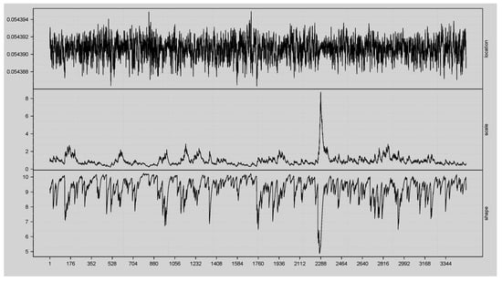
Figure 5. Time-varying parameter estimates of the fitted univariate GAS model with STD, showing the evolution of the conditional location, scale, and shape parameters.

3.2.3. Out-of-Sample Forecasts (Rolling Forecasts) of the Fitted GAS–STD Model

For the out-of-sample forecasts, we implement a rolling forecast procedure using the UniGASRoll() function in R. A moving window of 250 observations is used to generate forecasts. The models are re-estimated every 10 observations (RefitEvery = 10) using the most recent 250 data points (RefitWindow = "moving"), and a one-step-ahead forecast is generated at each step, ensuring dynamic updating of parameters.

Table 12 presents the first ten rolling forecasts produced by the GAS-STD model. Results include the conditional mean (location) being fairly stable over the forecasting period, changing in the range of $0.0525$. Conditional volatility (scale), however, changes more and spans from $0.6308$ to $0.8311$, reflecting dynamic model responses to changing market uncertainty. The estimated shape parameter is always considerably greater than 9, indicating that the fitted Student-t distribution has moderately heavy tails. This suggests the ability of the model to handle fat-tailed behaviour in the return distribution is essential in financial risk modelling. The forecasts indicate, however, that although the level of returns is stable around its mean value, volatility and tail heaviness exhibit considerable dynamics over time.

Table 12. First ten rolling forecasts of the fitted GAS–STD model.

Horizon	Location	Scale	Shape
$T+1$	$0.0525$	$0.6464$	$9.7908$
$T+2$	$0.0525$	$0.6403$	$9.8535$
$T+3$	$0.0525$	$0.7544$	$9.6885$
$T+4$	$0.0525$	$0.7429$	$9.7573$
$T+5$	$0.0525$	$0.6863$	$9.7715$
$T+6$	$0.0525$	$0.6421$	$9.7972$
$T+7$	$0.0525$	$0.6308$	$9.8567$
$T+8$	$0.0525$	$0.8311$	$9.2013$
$T+9$	$0.0525$	$0.7653$	$9.2525$
$T+10$	$0.0525$	$0.7087$	$9.3046$

The conditional location plot in Figure 6 illustrates the time-varying expected return of the JSE Top40 Index over the rolling forecast horizon. While the first ten forecast points remain constant at approximately $0.0525$, the long series of 250 points makes minimal fluctuations, with small upward and downward deviations from the mean level. These small movements are modest short-run trends in the expected return, which capture subtle directional changes in market sentiment without pronounced directional movements. Typically, the conditional mean is quite stable, consistent with low mean daily returns typical for equity indices.

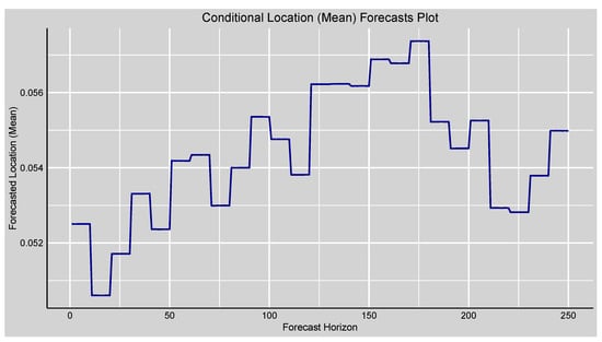
Figure 6. Forecasts plot of the forecasted conditional location (mean) of the fitted GAS-STD model.

The conditional scale (volatility) plot in Figure 7 displays the time series volatility of the returns and indicates considerable changes over the forecast period. Volatility initially falls a bit, then registers peaks, which correspond to instances of increased uncertainty and possible market tension. The remaining points show moderate levels of volatility, which correspond to fairly stable market conditions. These trends highlight the model’s strength in detecting short-run movements in risk, which is important for accurate risk determination and portfolio administration.

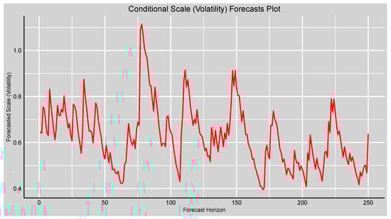
Figure 7. Forecasts plot of the forecasted conditional scale (volatility) of the fitted GAS–STD model.

The shape parameter curve in Figure 8 of the conditional shape, which reflects the Student’s t-distribution’s degrees of freedom, trends slightly above $9.7$ with some drops between 8 and 10. The distributions converge to normal as the shape parameter grows larger, and smaller values represent heavier tails. Volatility observed means that the return distributions predicted are generally well-approximated by a nearly normal distribution but periodically encounter bouts of heavier tails, which is valuable for the extreme return event modelling in risk analysis.

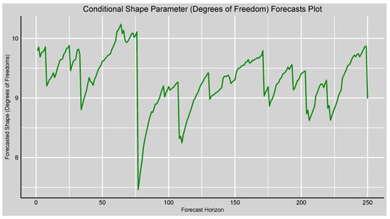
Figure 8. Forecasts plot of the forecasted conditional scale (volatility) of the fitted GAS–STD model.

Figure 9 shows the realised volatility against the forecasted conditional scale (volatility). The smoothed and more stable character of the forecasts of the conditional volatility is evident but succeeds in describing the overall patterns and volatility clusters fairly satisfactorily over the course of time. The surges in the higher volatility for the realised data near horizons 40, 100, and 200 are reflected in corresponding surges in the forecasted scale, though with lower amplitude. Such behaviour is consistent with the mission of volatility models, which anticipate explaining persistent dynamics and volatility clustering but not replicating every individual spike. These results indicate that the GAS–STD model provides an adequate explanation of conditional mean and volatility, as well as a stronger explanation of volatility dynamics than of return levels.

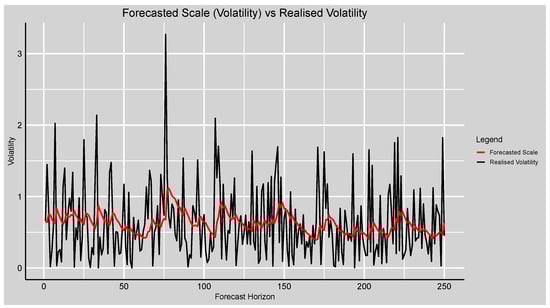
Figure 9. Plot of the forecasted conditional scale (volatility) versus realised volatility of the fitted GAS–STD model.

Table 13 displays some of the rolling risk forecasts of the 5% value-at-risk (VaR) and expected shortfall (ES) from the GAS–STD model. Both VaR and ES are invariably negative in the results, which reflects the model’s risk estimation in the return series from the downside. VaR estimates from approximately $-1.0925$ to $-1.4672$ indicate the estimated tail risk at the $5\%$ confidence level, while ES estimates from $1.4704$ to $-1.9787$ indicate the mean loss in the tail 5% of situations. As expected, ES is more negative than VaR, confirming its characteristic as a coherent risk measure giving a closer estimate of tail risk than VaR. Figure 10 further illustrates these numerical results by displaying the full rolling paths of the $5\%$ VaR and ES across the forecast horizon. These risk measures exhibit strong time variation, with fluctuations that correspond to periods of heightened volatility. As theory would expect, ES is below VaR for all forecast horizons, as it accounts for the severity of losses beyond the VaR level. Growing differences between the two measures at more volatile times (e.g., past forecast horizons of 80, 150, and 220) again illustrate how ES is reacting more sensitively to extreme negative returns. Table 13 and Figure 10 provide a neat image of the tail risk behaviour of the GAS–STD model in favour of the idea that it is essential to utilise both VaR and ES for complete risk assessment.

Table 13. Rolling Risk Forecasts from the 5% VaR and ES.

VaR (5%)	ES (5%)
−1.1215	−1.5098
−1.1098	−1.4935
−1.3192	−1.7742
−1.2974	−1.7443
−1.1943	−1.6069
−1.1137	−1.4993
−1.0925	−1.4704
−1.4672	−1.9787
−1.3460	−1.8160
−1.2418	−1.6760

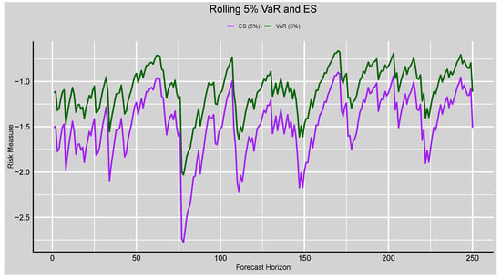
Figure 10. Rolling Risk Forecasts plot from the 5% VaR and ES.

Table 14 shows the forecast measures of performance for both the conditional location (mean) and conditional scale (volatility) of the estimated GAS–STD model. It is revealed from the findings that there are lower errors in scale forecasts than in the location forecasts based on lower RMSE ($0.5373$ vs. $0.8055$) and MAE ($0.4197$ vs. $0.6233$) values. This suggests that the model is more appropriate to predict volatility dynamics than return levels, which is consistent with the typical dynamics of financial time series where volatility is more persistent and, hence, more predictable than returns. However, the MAPE measures for the two series are very high $(184.5542\%$ for location and $1083.5356\%$ for scale), as one would anticipate, because returns and volatility occasionally assume values close to zero, thereby inflating percentage-error measures. Finally, the MASE values indicate that both forecasts are quite good relative to a naïve baseline, with values close to but below unity ($0.7026$ for the location and $0.7464$ for the scale). These results indicate that the GAS–STD model produces optimal volatility predictions with excellent persistence in its volatility, whereas conditional mean predictions are poorer due to the inherent volatility uncertainty of financial return levels.

Table 14. Forecast accuracy metrics for conditional location and scale of the fitted GAS–STD model.

Accuracy Measure	Location	Scale
MASE	0.7026	0.7464
RMSE	0.8055	0.5373
MAE	0.6233	0.4197

The backtest results of the 5% value-at-risk (VaR) model in Table 15 are discovered to have adequate predictive power. The Kupiec unconditional coverage test (LRuc) yielded a test statistic of $0.0400$ and a p-value of $0.8414$, failing to reject the null hypothesis of correct unconditional coverage. This is a pointer that the observed rate of violations is statistically consistent with the expected rate at the specified confidence level. The Christoffersen conditional coverage test (LRcc) produced a statistic of $3.5026$ and a p-value of $0.1735$, not rejecting once more the null hypothesis of adequate conditional coverage. It therefore follows that VaR violations are both time series independent and at the correct frequency. The actual/expected exceedance ratio (AE) was $0.9673$, very close to unity, which testifies that the number of exceedances is very close to the model’s theoretical expectation. The Acerbi–Szekely (AD) tests provided ADmean = $0.4723$ and ADmax = $1.6313$, which are both low values signifying no systematic underestimation or overestimation of the tail losses. The dynamic quantile (DQ) test statistic value of $9.3557$ and p-value of $0.2281$ also signify the absence of significant autocorrelation in exceedances and that the model is good in the detection of the time dependence of the tail events. Finally, the observed loss function value of $0.1097$ is relatively low, indicating high predictive precision in the left tail of the distribution. Overall, these diagnostic results individually suggest that the VaR model reflects high statistical fitness and credibility in quantifying downside risk at the 5% level of the out-of-sample period.

Table 15. Backtest Results for the 5% VaR Model.

Test	Statistic	p-Value
Kupiec Unconditional Coverage (LRuc)	0.0400	0.8414
Christoffersen Conditional Coverage (LRcc)	3.5026	0.1735
Actual/Expected (AE) Ratio	0.9673	–
ADmean	0.4723	–
ADmax	1.6313	–
Dynamic Quantile (DQ)	9.3557	0.2281
Loss Function	0.1097	–

As shown in Table 16, the value-at-risk (VaR) backtests indicate that both the skewed Student-t (SSTD) and asymmetric Student-t (AST) generalised autoregressive score (GAS) models produce statistically adequate 5% VaR forecasts. The Kupiec unconditional coverage (LRuc) p-values (0.5802 for SSTD and 0.2730 for AST) and Christoffersen conditional coverage (LRcc) p-values (0.1860 for SSTD and 0.1571 for AST) suggest correct unconditional coverage and no evidence of clustering of violations. The Engle–Manganelli dynamic quantile (DQ) p-values (0.2342 for SSTD and 0.3613 for AST) confirm no dynamic misspecification in the conditional quantile process. Actual/expected (AE) ratios of 0.9104 (SSTD) and 0.8250 (AST) indicate slightly conservative forecasts but remain close to the nominal level. Overall, both asymmetric distributions satisfy the standard VaR adequacy criteria, supporting the robustness of the results reported in Table 16.

Table 16. GAS Model: Information Criteria and Essential VaR Backtests (SSTD vs. AST).

Metric/Test	GAS-SSTD	GAS-AST
AIC	10,190.46	10, 203.18
BIC	10,264.44	10,283.32
LRuc p-value	0.5802	0.2730
LRcc p-value	0.1860	0.1571
DQ p-value	0.2342	0.3613
AE	0.9104	0.8250

3.2.4. Simulation-Based Tail Risk Analysis

In this research, there were a total of 10,000 observations simulated from the GAS–STD model for every fixed value of shape parameter or degrees of freedom, $\nu =(5,8,10,15,20,25,30)$. Table 17 displays kurtosis of simulated data, and it is clear that lower values of $\nu$ create series with heavier tails, as indicated by higher total kurtosis (e.g., $7.32$ for $\nu =5$), while higher values of $\nu$ create distributions with kurtosis closer to the Gaussian standard of 3 (e.g., $3.14$ for $\nu =30$). This finding is also indicated by the QQ plots in Figure 11, comparing the quantiles of the simulated data with those of a standard normal distribution. For lower values of $\nu$, i.e., $5,8$, and 10, the QQ plots indicate strong deviations from the 45-degree line at the tails, confirming strong leptokurtic behaviour. By contrast, larger values of $\nu$, especially $20,25,$ and 30, fall exactly on the theoretical line, showing distributions that are close to normal. This evidence suggests that smaller degrees of freedom produce greater tail heaviness, with $\nu =5$ being the best choice when extreme tail behaviour is assigned greatest significance. This option represents the largest leptokurtosis, particularly for the simulation of financial asset returns and estimation of the risk of rare extreme market events.

Table 17. Total kurtosis values of simulated data generated from the GAS-STD model under fixed shape parameter or degrees of freedom ($\nu =5,8,10,15,20,25,30$).

Degrees of Freedom ($\mathit{\nu }$):	$\mathit{\nu }=5$	$\mathit{\nu }=8$	$\mathit{\nu }=10$	$\mathit{\nu }=15$	$\mathit{\nu }=20$	$\mathit{\nu }=25$	$\mathit{\nu }=30$
kurt value:	7.3197	4.4795	3.9495	3.4740	3.3005	3.1968	3.1401

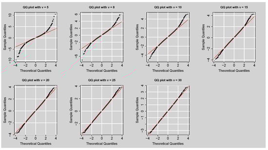
Figure 11. QQ plots of simulated data from the GAS–STD model under fixed shape parameter or degrees of freedom values ($\nu =6,8,10,15,20,25,30$).

Figure 12 represents the histogram of simulated data together with the estimated 5% value-at-risk (VaR) and expected shortfall (ES) thresholds. Most of the distribution is concentrated around zero, indicating typical behaviour of financial return series that fluctuate around the mean. However, fat tails also exist, as indicated by the presence of extreme negative observations in the left tail. The vertical dashed red lines represent the 5% VaR and ES levels, which were calculated to be $-1.8032$ and $-2.6702$, respectively. The 5% VaR provides the cutoff point after which the worst 5% of losses lie, whereas the ES is an estimate of the average loss given that it crosses this threshold. The locations of these thresholds also readily demonstrate that although infrequent instances of catastrophic downside loss are themselves fairly frequent, their size is substantial, with mean losses (ES) even larger than the VaR cutoff. This finding confirms the presence of leptokurtosis in the simulated data and the necessity of modelling fat-tailed distributions to optimally describe the risk profile of financial returns.

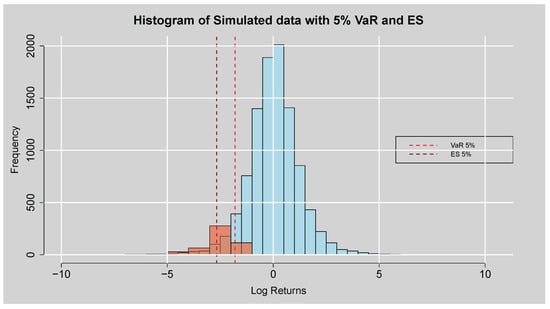
Figure 12. Histogram plot of the simulated data with 5% Var and ES.

Figure 13 plots the time series plot of the simulated data across 10,000 observations with the $5\%$ VaR level plotted in red. The simulated data exhibit large fluctuations about the zero mean, with some sharp spikes indicating instances of very high variation. The red points that fall below the $5\%$ VaR level are those instances in which losses exceeded the risk threshold, an instance of very high negative returns. These excesses are randomly distributed throughout the sample, suggesting the existence of tail risk in the simulated distribution. The frequency and diversity of these breaches suggest that the model captures both the middle dynamics of return behaviour and fairly accurately reflects the fat-tailed nature of financial returns, which is fundamental for risk management applications.

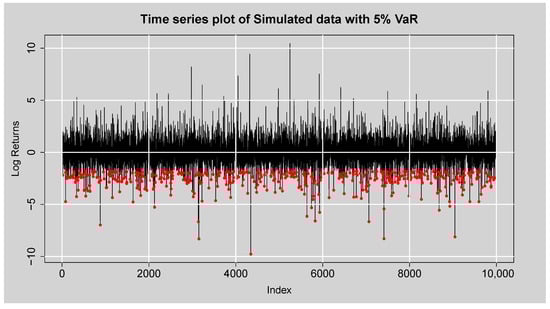
Figure 13. Time series plot of the simulated data with 5% VaR.

3.2.5. Forecasts Comparisons of the Standalone ARMA(3,2)–EGARCH(1,1) Model, GAS–STD Model, and ARMA(3,2)–EGARCH(1,1)–XGBoost Hybrid Model

Table 18 presents the forecast accuracy statistics of the ARMA(3,2)–EGARCH(1,1), GAS–STD, and ARMA(3,2)–EGARCH(1,1)–XGBoost models. For all the measures, the ARMA(3,2)–EGARCH(1,1)–XGBoost model performs better than the remaining models, with the lowest MASE, RMSE, and MAE. The ARMA(3,2)–EGARCH(1,1) model comes in second overall, and the GAS–STD model has comparatively higher errors in most measures. These results imply that inclusion of the XGBoost module drastically improves predictive power, catching nuances the fully parametric models may not.

Table 18. Forecast Accuracy Measures for ARMA(3,2)–EGARCH(1,1), GAS–STD, and ARMA(3,2)–EGARCH(1,1)–XGBoost Models.

Accuracy Measure	ARMA(3,2)–EGARCH(1,1)	GAS–STD	ARMA(3,2)–EGARCH(1,1)–XGBoost
MASE	0.6827	0.7464	0.0534
RMSE	1.0845	0.5373	0.1386
MAE	0.8176	0.4197	0.0595

Table 19 reports the bootstrap root mean squared error (RMSE) and 95% percentile confidence intervals for all competing volatility models. The hybrid model achieves the lowest RMSE (0.1386), indicating superior predictive accuracy compared with both the ARMA(3,2)–EGARCH(1,1) (RMSE = 1.1282) and GAS-STD (RMSE = 0.5361) models. The corresponding confidence intervals show little overlap, reinforcing the hybrid model’s strong performance.

Table 19. Bootstrap RMSE and 95% Confidence Intervals for Competing Models.

Model	RMSE	95% CI (Lower)	95% CI (Upper)
Hybrid	0.1386	0.0872	0.1890
ARMA(3,2)–EGARCH(1,1)	1.1282	1.0378	1.2181
GAS–STD	0.5361	0.4728	0.6041

The Diebold-Mariano (DM) test results in Table 20 provide further evidence of significant predictive differences. The negative confidence intervals for “Hybrid vs. ARMA(3,2)–EGARCH(1,1)” and “Hybrid vs. GAS–STD” confirm that the hybrid model yields statistically smaller forecast errors, while the positive interval for “ARMA(3,2)–EGARCH(1,1) vs. GAS–STD” indicates that the GAS–STD model outperforms ARMA–EGARCH. The bootstrap results highlight the robustness of the hybrid model’s superior forecasting ability.

Table 20. Bootstrap 95% Confidence Intervals for Diebold-Mariano (DM) Statistics.

Model Comparison	95% CI (Lower)	95% CI (Upper)
Hybrid vs. ARMA(3,2)–EGARCH(1,1)	−22.53	−19.92
Hybrid vs. GAS–STD	−15.48	−9.91
ARMA(3,2)–EGARCH(1,1) vs. GAS–STD	9.56	12.16

The Full Diebold-Mariano (DM) test results in Table 21 show that all pairwise comparisons yield p-values below 0.01, indicating statistically significant differences in predictive accuracy among the models. In each comparison, the hybrid ARMA(3,2)–EGARCH(1,1)–XGBoost model achieves consistently lower forecast loss relative to both models (ARMA(3,2)–EGARCH(1,1) and GAS–STD). This means that the hybrid model provides significantly superior out-of-sample forecast performance across the evaluation period.

Table 21. Full Diebold-Mariano (DM) test p-value matrix for competing models.

	Hybrid	ARMA(3,2)–EGARCH(1,1)	GAS–STD
Hybrid	–	0.000000	0.002648
ARMA(3,2)–EGARCH(1,1)	0.000000	–	0.000000
GAS–STD	0.002648	0.000000	–

The Model Confidence Set (MCS) results in Table 22 further confirm this finding: only the hybrid model remains within the superior set at the 5% significance level, while both ARMA(3,2)–EGARCH(1,1) and GAS–STD are eliminated during the sequential testing process. Overall, the DM and MCS procedures jointly indicate that the hybrid model statistically dominates its competitors in terms of volatility forecast accuracy and robustness.

Table 22. Model Confidence Set (MCS) procedure results using the $T_{\max }$ statistic.

Model	RankM	${\mathit{v}}_{\mathit{M}}$	MCSM	RankR	${\mathit{v}}_{\mathit{R}}$	MCSR
Hybrid	1	−14.53997	1	1	-14.53997	1
ARMA(3,2)–EGARCH(1,1)	2	–	0	2	–	0
GAS–STD	3	–	0	3	–	0

The empirical scores plot displayed in Figure 14 presents a comparison between the ARMA(3,2)–EGARCH(1,1) model and the hybrid ARMA(3,2)–EGARCH(1,1)–XGBoost model based on Murphy diagrams. The results confirm that the hybrid model has lower empirical scores over a wider parameter space compared to the standalone ARMA(3,2)–EGARCH(1,1). The implication is that the hybrid model provides more accurate volatility forecasts, particularly for the right tail of the distribution, where it provides a more sustained and smoother reduction in scores. Conversely, the ARMA(3,2)–EGARCH(1,1) model by itself does not have such a steep peak but a more limited fall, which reflects worse performance in explaining volatility dynamics at longer horizons. Figure 15 also substantiates this conclusion by presenting the difference between the two models’ scores. The negative values of the score differences across most of the parameter domain indicate that the hybrid model outperforms the standalone ARMA(3,2)–EGARCH(1,1). The confidence band reinforces the robustness of this finding, as it remains below zero for a substantial portion of the parameter range. Only in the very narrow region around the origin do the two models exhibit comparable performance, after which the hybrid model clearly dominates. These results highlight the predictive gain obtained by combining the traditional ARMA(3,2)–EGARCH(1,1) specification with the nonlinear learning ability of XGBoost, confirming that the hybrid framework provides superior predictive accuracy in volatility forecasting.

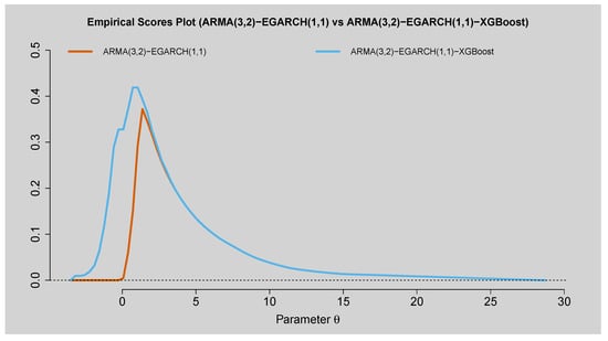
Figure 14. Empirical Scores Plot of ARMA(3,2)–EGARCH(1,1) vs. ARMA(3,2)–EGARCH(1,1)–XGBoost.

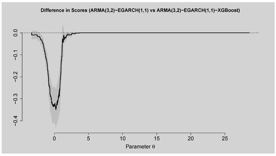
Figure 15. Difference in Scores Plot of ARMA(3,2)–EGARCH(1,1) vs. ARMA(3,2)–EGARCH(1,1)–XGBoost.

Figure 16 and Figure 17 show the predictive capability of the GAS–STD model compared to the ARMA(3,2)–EGARCH(1,1)–XGBoost model. The empirical scores plot shows that both models reach their peak in roughly the same region but that the ARMA(3,2)–EGARCH(1,1)–XGBoost scores higher across the entire parameter set, which means better predictive capability. Difference in scores plot confirms this, as the curve is below zero for nearly all periods, indicating that the hybrid ARMA(3,2)–EGARCH(1,1)–XGBoost model is better in all horizons than GAS–STD, particularly the short horizon. At higher horizons, differences tend towards zero, indicating similar performance between both models.

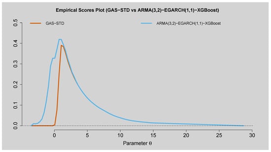
Figure 16. Empirical Scores Plot of GAS–STD vs. ARMA(3,2)–EGARCH(1,1)–XGBoost.

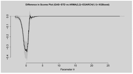
Figure 17. Difference in Scores Plot of GAS–STD vs. ARMA(3,2)–EGARCH(1,1)–XGBoost.

Figure 18 presents the empirical scores plot comparing the performance of the ARMA(3,2)–EGARCH(1,1) model to that of the GAS–STD model. The plots validate that both models begin with the same trajectory, but with the ARMA(3,2)–EGARCH(1,1) having greatly reduced scores within the parameter space, reflecting better predictability, especially for large parameter values of $\theta$. On the contrary, the GAS–STD model increases more steeply and subsequently converges rapidly towards zero, indicative of a diminished ability to forecast beyond the short-run horizon. The plot of the score difference in Figure 19 lends additional support to this conclusion. The positive differences indicated in the difference curve, particularly at the lower range of $\theta$, attest that ARMA(3,2)–EGARCH(1,1) is superior to the GAS–STD model. The confidence band supports the strong evidence for the result, since it remains positive for the majority of the relevant domain. Beyond the small range, the differences converge and finally centre on zero, demonstrating comparable long-horizon performance by both models. The overall results confirm that the ARMA(3,2)–EGARCH(1,1) model is more predictive in the short to medium term than the GAS–STD model, with both models demonstrating similar performance over longer horizons.

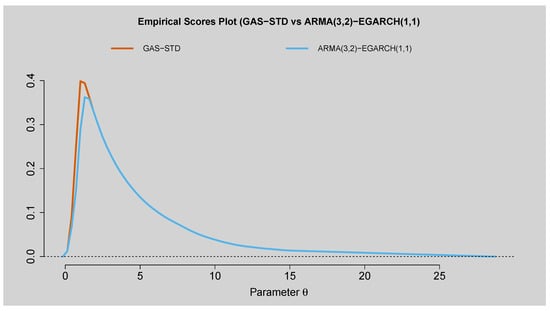
Figure 18. Empirical Scores Plot of GAS–STD vs. ARMA(3,2)–EGARCH(1,1).

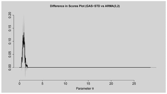
Figure 19. Difference in Scores Plot of GAS–STD vs. ARMA(3,2)–EGARCH(1,1).

3.3. Comparative Analysis with MOEX Index

The summary statistics given in Table 23 show a divergence in the risk and return profiles of the two markets, JSE Top40 and the MOEX indices. In terms of performance, the JSE Top40 shows a marginally higher average daily return of 0.034% compared to the MOEX’s 0.011%. However, this slight advantage is overshadowed by the difference in risk. The MOEX is more volatile, with a standard deviation of 1.51%, which is approximately 33% higher than the JSE Top40’s 1.14%, indicating much greater day-to-day price fluctuation for its investors.

Table 23. Summary Statistics of both JSE Top40 and MOEX Log-Returns.

Index	Mean	SD	Min	Max	Skewness	Kurtosis
JSE Top40	0.03396229	1.135643	−10.45042	9.056979	−0.2890831	9.332561
MOEX	0.01091726	1.508611	−40.46744	18.261952	−5.2568647	151.912160

The prevalence of extreme events further evidences this heightened risk. The MOEX has experienced far more severe market movements, with a maximum negative return of −40.47% and a positive return of 18.26%, both of which dwarf the extremes seen on the JSE. The shape of the return distributions provides deeper insight: both indices show negative skewness, but the MOEX’s profoundly negative value highlights a propensity for severe crashes. Furthermore, while the JSE exhibits “fat-tailed" leptokurtic behaviour, the MOEX’s very high kurtosis confirms an extreme incidence of outlier events. This shows that the MOEX is a riskier market, offering lower average returns while being exposed to dramatically higher volatility and extreme event risk.

The GAS–STD model parameter estimates shown in Table 24 show distinct dynamics of the two markets. Both markets have highly persistent volatility, with parameters ($b_2$) near 1. MOEX (0.987) is slightly more persistent than the JSE (0.974). MOEX’s volatility is also more reactive to new shocks, shown by its higher $a_2$ (0.188 vs. 0.174). For tail behaviour, MOEX has a much larger $a_3$ (6.55 vs. 1.80) and a smaller $b_3$ (0.62 vs. 0.87). This means its tail shape is more reactive to shocks and less persistent. MOEX’s more negative ${\kappa }_3$ (−1.08 vs. −0.28) confirms a consistently more negatively skewed distribution. Inference shows MOEX’s tail-risk dynamics are far more reactive and volatile, while the JSE exhibits more stable distributional dynamics.

Table 24. Parameter Estimates of the fitted GAS-STD.

Parameter	JSE Top40 Estimate	MOEX Estimate
${\kappa }_1$	0.03924	0.03589
${\kappa }_2$	−0.00442	0.00011
${\kappa }_3$	−0.27663	−1.08251
$a_1$	9.99 $\times {10}^{-7}$	1.04 $\times {10}^{-6}$
$a_2$	0.17429	0.18754
$a_3$	1.79702	6.54908
$b_1$	0.37173	0.47057
$b_2$	0.97438	0.98705
$b_3$	0.87096	0.62455

The model’s goodness-of-fit is worse for the MOEX, as indicated by its higher AIC and BIC values, and its significantly lower log-likelihood (LLK), as shown in Table 25. This is expected, as the MOEX’s data, with their extreme outliers, are much more difficult for any model to fit neatly.

Table 25. In-sample fit (AIC, BIC, LLK) of GAS–STD.

	Market
	JSE	MOEX
AIC	10,676.876	11,407.965
BIC	10,732.826	11,463.944
LLK	−5329.438	−5694.983

The scatter plot of the JSE Top 40 vs. MOEX, given in Figure 20, shows a non-linear relationship between the two markets’ daily returns, suggesting a low correlation and potential for diversification benefits.

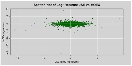
Figure 20. Scatter Plot of Log-Returns: JSE vs. MOEX.

The time series plot of the log-returns in Figure 21 show that the JSE Top40 returns oscillate within a relatively stable band. In contrast, the MOEX returns are punctuated by several massive spikes, both positive and negative, corresponding to its extreme min/max values, as shown in Table 23.

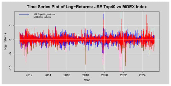
Figure 21. Time series plot of log-returns of the JSE Top40 and MOEX indices.

The 20-day volatility of the MOEX consistently runs above that of the JSE Top40, as shown in Figure 22, with pronounced peaks during periods of crisis that far exceed any volatility spikes seen in the South African market.

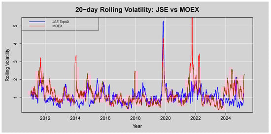
Figure 22. 20-day Rolling Volatility: JSE vs. MOEX.

The scale forecasts given in Table 26 represent future volatility. Across all forecast horizons ($T+1 \mathrm{to} T+10$), the scale forecast for the MOEX is consistently and substantially higher than for the JSE Top40, often by a factor of 3 or 4. This confirms the model’s conclusion that the future volatility environment for the MOEX is predicted to remain significantly more turbulent than for the JSE. A plot of the scale forecasts is given in Figure 23.

Table 26. Scale forecasts comparisons.

Horizon	Scale_JSE	Scale_MOEX
$T+1$	0.414	1.499
$T+2$	0.411	1.461
$T+3$	0.398	1.307
$T+4$	0.409	1.634
$T+5$	0.565	1.664
$T+6$	0.592	1.541
$T+7$	0.551	2.100
$T+8$	0.535	2.049
$T+9$	0.677	1.959
$T+10$	0.676	1.757

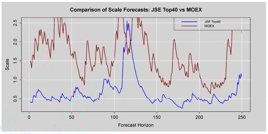
Figure 23. Comparison of Scale Forecasts: JSE Top40 vs. MOEX.

The GAS–STD model validates that the MOEX is not only historically more volatile but is also expected to remain so in the immediate future. The poorer model fit for the MOEX underscores the challenge of modelling such a chaotic market.

4. Discussion

The empirical results in Section 3 demonstrate that the Student-t distribution of the GAS model (GAS–STD) provides the best fit for the JSE Top40 Index returns among the conditional distributions considered. Table 6 comparison measures show that the GAS–STD produces the lowest AIC (10,188.142) and BIC (10,243.626) values, which means that it maximises goodness-of-fit and parsimony compared to the Gaussian, skew-Gaussian, or asymmetric forms. The parameter estimates also detect considerable persistence of location and scale dynamics with coefficients $a_2$ and $b_2$, statistically significant at 1%. This confirms that past volatility has a strong effect on current volatility, a common feature of financial return series. The findings of the shape parameter are that the return distribution is time-varying in terms of tail heaviness and that there are indications of episodes of extreme kurtosis during times of market distress. A diagnostic examination of the estimated GAS-STD model also confirms that it is a density forecast. Both the PIT histogram in Figure 4 and the uniform scores in Table 10 indicate that the model produces well-calibrated predictive densities, although skewness tests do identify an unexplained residual asymmetry. Consequently, density backtests such as normalised log score (1.1932) and uniform PIT score (0.4417) in Table 10 attain good forecast accuracy through balanced performance in the centre and tails of the distribution. Forecasting evaluation further indicates that GAS–STD outperforms in the capture of volatility dynamics over mean returns. Rolling forecasts show the conditional mean is generally level, such as in the martingale property of asset returns, while forecast volatility shows clear clustering that tracks very closely with realised volatility. Accuracy measures for the forecasts verify that RMSE (0.5373) for the volatility forecast is substantially lower than for mean return levels (which is 0.8055). These findings underscore that the GAS model works best when the modelling objective is forecasting volatility rather than mean returns prediction. Risk management analysis incorporating value-at-risk (VaR) and expected shortfall (ES) concludes that the GAS-STD yields plausible downside risk estimates. Both 5% VaR and ES forecasts dynamically adapt to clusters of volatility, and backtests confirm good performance: the Kupiec test for unconditional coverage ($p=0.8414$) and the Christoffersen test for conditional coverage ($p=0.1735$) fail to reject good coverage, and the dynamic quantile test ($p=0.2281$) further confirms good dynamic exceedance behaviour. Such findings demonstrate the GAS–STD to be an effective method of quantifying tail risk in equity indices. These are supported by simulation studies in demonstrating the impact of the shape parameter $\nu$ on tail behaviour. Small values of $\nu$ ($\nu =5$) yield levels of total kurtosis greater than 7 that characterise heavy tails, whereas larger ones ($\nu =30$) converge towards the Gaussian benchmark point. This is the kind of behaviour that captures the leptokurtic nature of financial returns, an essential requirement when modelling extreme risk. Comparison with other models, however, shows that although GAS–STD is superior in density and risk forecasting, the hybrid model that includes machine learning surpasses it in point forecast accuracy. The ARMA(3,2)–EGARCH(1,1)–XGBoost model has much lower RMSE (0.1386) than GAS–STD, and full DM and MSC tests in Table 21 and Table 22 confirm that the hybrid forecasts are better. Murphy diagrams in Figure 14, Figure 15, Figure 16, Figure 17, Figure 18 and Figure 19 also show that the hybrid model surpasses GAS–STD and stand-alone ARMA(3,2)–EGARCH(1,1) at all forecast horizons. These results highlight that model choice depends on the purpose of forecasting: GAS–STD for risk measures and density and the hybrid model for short-horizon volatility forecasts.

A comparative analysis was then conducted between the JSE Top 40 index and the Russian all-share index, the MOEX. The JSE Top 40 presents itself as a relatively stable emerging market, characterised by moderate returns, lower volatility, and less severe tail events. Its dynamics are persistent but less reactive, making it a potentially less risky investment within the emerging market universe.

The MOEX is characterised by high instability. It exhibits lower average returns, dramatically higher volatility, and an extreme susceptibility to catastrophic crashes. Its market dynamics are highly reactive and persistent, leading to a forecast of continued elevated risk. The differences, particularly in extreme event risk, are likely due to the distinct geopolitical, commodity-dependent, and structural economic factors influencing the Russian market, which have historically led to greater turbulence compared to the South African market.

5. Conclusions

This study focused on volatility modelling of the JSE Top40 Index using the GAS framework as the primary method, while ARMA(3,2)–EGARCH(1,1) and the hybrid ARMA(3,2)–EGARCH(1,1)–XGBoost models were used as benchmarks for comparison. It is shown that GAS–STD provides the most suitable specification within the GAS family and excels in density calibration, tail risk forecasting, and VaR/ES backtesting. Its attractiveness lies in its capability to model volatility persistence and heavy-tailed distributions, making it a suitable match for financial risk management. However, the hybrid ARMA(3,2)–EGARCH(1,1)–XGBoost is more accurate than GAS and ARMA(3,2)-EGARCH(1,1) in terms of point forecasting accuracy, as corroborated by forecast error measures and DM and MSC tests in Table 21 and Table 22. The results suggest that the GAS model ought to be preferred for density-based applications such as risk estimation and stress testing, whereas the hybrid approach is more appropriate for short-term forecasting exercises. In practice, the GAS model would be of greater utility to regulators and risk managers requiring adequate density forecasts for stress testing, capital allocation, and value-at-risk (VaR) estimation. The hybrid GARCH-XGBoost model is more suited for algorithmic traders and portfolio managers seeking short-horizon price prediction and trading directions. These findings could be expanded to other emerging markets with identical volatility clustering and nonlinearity patterns like those of the JSE, but in developed economies with greater liquidity, model calibration, and performance could vary with less persistence and better information flow.

Although this study offers valuable insights into volatility modelling for the JSE Top40 Index, several limitations warrant consideration. The scope is limited to a single emerging market and focuses exclusively on daily return data. The analysis evaluates only the GAS framework and selected hybrid ARMA(3,2)–EGARCH(1,1)–XGBoost models, leaving other sophisticated approaches such as regime-switching MS-GARCH, SVR–GARCH, NN–GARCH, or MIDAS models incorporating fundamental variables unexamined. Additionally, the models’ predictive performance may differ in markets characterised by varying liquidity, persistence, or information dissemination patterns. Future research should examine skewed GAS distributions, hybrid GAS models, and multivariate extensions to facilitate cross-market volatility spillovers.

References

- Acerbi, C., & Tasche, D. (2002). On the coherence of expected shortfall. Journal of Banking & Finance, 26(7), 1487–1503. [Google Scholar] [CrossRef]
- Alanya-Beltran, W. (2022). Modelling stock returns volatility with dynamic conditional score models and random shifts. Finance Research Letters, 45, 102–121. [Google Scholar] [CrossRef]
- Ardia, D., Boudt, K., & Catania, L. (2019). Generalized autoregressive score models in R: The GAS package. Journal of Statistical Software, 88, 1–28. [Google Scholar] [CrossRef]
- Artzner, P., Delbaen, F., Eber, J.-M., & Heath, D. (1999). Coherent measures of risk. Mathematical Finance, 9(3), 203–228. [Google Scholar] [CrossRef]
- Babatunde, O., Folorunso, S., & Saliu, F. (2021). Comparative forecasting performance of GARCH and GAS models in the Stock Price Traded on Nigerian Stock Exchange. International Journal of Mathematical Modelling & Computations, 11(2 SPRING). Available online: https://www.researchgate.net/publication/354664008_Comparative_Forecasting_Performance_of_GARCH_and_GAS_Models_in_the_Stock_Price_Traded_on_Nigerian_Stock_Exchange (accessed on 9 September 2025).
- Bauwens, L., Laurent, S., & Rombouts, J. V. K. (2006). Multivariate GARCH models: A survey. Journal of Applied Econometrics, 21(1), 79–109. [Google Scholar] [CrossRef]
- Bildirici, M., & Ersin, O. (2016). Markov switching artificial neural networks for modelling and forecasting volatility: An application to gold market. Procedia Economics and Finance, 38, 106–121. [Google Scholar] [CrossRef]
- Bollerslev, T. (1986). Generalized autoregressive conditional heteroskedasticity. Journal of Econometrics, 31(3), 307–327. [Google Scholar] [CrossRef]
- Chaudhary, S., & Uprety, D. (2024). Hybrids ARIMA-ANN models for GDP forecasting in Nepal. NRB Economic Review, 35(1–2), 22–53. [Google Scholar]
- Chen, T., & Guestrin, C. (2016, August 13–17). XGBoost: A scalable tree boosting system. Proceedings of the 22nd ACM SIGKDD International Conference on Knowledge Discovery and Data Mining (pp. 785–794), San Francisco, CA, USA. [Google Scholar] [CrossRef]
- Creal, D., Koopman, S. J., & Lucas, A. (2013). Generalized autoregressive score models with applications. Journal of Applied Econometrics, 28(5), 777–795. [Google Scholar] [CrossRef]
- Diebold, F. X., & Mariano, R. S. (1995). Comparing predictive accuracy. Journal of Business & Economic Statistics, 13(3), 253–263. [Google Scholar] [CrossRef]
- Engle, R. F. (1982). Autoregressive conditional heteroscedasticity with estimates of the variance of United Kingdom inflation. Econometrica: Journal of the Econometric Society, 50(4), 987–1007. [Google Scholar] [CrossRef]
- Eniayewu, P. E., Tukura, G. S., Joshua, J. D., Tuapreghe, B., & Yusuf, U. (2024). Forecasting exchange rate volatility with monetary fundamentals: A GARCH-MIDAS approach. Scientific African, 23, e01023. [Google Scholar] [CrossRef]
- Fang, T., Lee, T. H., & Su, Z. (2020). Predicting the long-term stock market volatility: A GARCH-MIDAS Model with variable selection. Journal of Empirical Finance, 58, 36–49. [Google Scholar] [CrossRef]
- Garai, S., Paul, R. K., Yeasin, M., & Paul, A. P. (2024). CEEMDAN-based hybrid machine learning models for time series forecasting using MARS algorithm and PSO-optimization. Neural Processing Letters, 56, 92. [Google Scholar] [CrossRef]
- Glosten, L. R., Jagannathan, R., & Runkle, D. E. (1993). On the relation between the expected value and the volatility of the nominal excess return on stocks. Journal of Finance, 48(5), 1779–1801. [Google Scholar] [CrossRef]
- Harvey, A. C. (2013). Dynamic models for volatility and heavy tails: With applications to financial and economic time series. Cambridge University Press. [Google Scholar] [CrossRef]
- Harvey, D., Leybourne, S., & Newbold, P. (1997). Testing the equality of prediction mean squared errors. International Journal of Forecasting, 13(2), 281–291. [Google Scholar] [CrossRef]
- Jefferis, K., & Smith, G. (2005). The changing efficiency of African Stock Markets. South African Journal of Economics, 73(1), 54–67. [Google Scholar] [CrossRef]
- Junior, P. O., & Alagidede, I. (2020). Risks in emerging markets equities: Time-varying versus spatial risk analysis. Physica A: Statistical Mechanics and Its Applications, 542, 123–474. [Google Scholar] [CrossRef]
- Lazar, E., & Xue, X. (2020). Forecasting risk measures using intraday data in a Generalized Autoregressive Score (GAS) framework. International Journal of Forecasting, 36(3), 1057–1072. [Google Scholar] [CrossRef]
- Maingo, I., Ravele, T., & Sigauke, C. (2025a). A fusion of statistical and machine learning methods: GARCH-XGBoost for improved volatility modelling of the JSE Top40 index. International Journal of Financial Studies, 13(3), 155. [Google Scholar] [CrossRef]
- Maingo, I., Ravele, T., & Sigauke, C. (2025b). Volatility modelling of the Johannesburg Stock Exchange all share index using the family GARCH model. Forecasting, 7(2), 16. [Google Scholar] [CrossRef]
- McNeil, A. J., Frey, R., & Embrechts, P. (2005). Quantitative risk management: Concepts, techniques and tools. Princeton University Press. Available online: https://www.riskbooks.com/ (accessed on 25 September 2025).
- Nadarajah, S., Mba, J. C., Ravonimanantsoa, N. M., & Ratolojanahary, H. T. J. E. (2025). Empirical calibration of XGBoost model hyperparameters using the Bayesian optimisation method: The case of bitcoin volatility. Journal of Risk and Financial Management, 18(9), 487. [Google Scholar] [CrossRef]
- Nelson, D. B. (1991). Conditional heteroskedasticity in asset returns: A new approach. Econometrica, 59(2), 347–370. [Google Scholar] [CrossRef]
- Opschoor, A., Janus, P., Lucas, A., & Van Dijk, D. (2018). New HEAVY models for fat-tailed realized covariances and returns. Journal of Business & Economic Statistics, 36(4), 643–657. [Google Scholar] [CrossRef]
- Rockafellar, R. T., & Uryasev, S. (2000). Optimization of conditional value-at-risk. Journal of Risk, 2(3), 21–41. [Google Scholar] [CrossRef]
- Sun, H., & Yu, B. (2020). Forecasting financial returns volatility: A GARCH-SVR model. Computational Economics, 55(2), 451–471. [Google Scholar] [CrossRef]
- Venter, P. J., & Mare, E. (2020). GARCH option pricing models in a South African equity context. ORiON: Journal of the Operational Research Society of Southern Africa, 36(1), 1–17. [Google Scholar] [CrossRef]
- Yaya, O. S., Bada, A. S., & Atoi, V. N. (2016). Volatility in the Nigerian Stock Market: Empirical application of Beta-t-GARCH variants. CBN Journal of Applied Statistics, 7(2), 27–48. [Google Scholar]
- Zhao, P., Zhu, H., NG, W. S. H., & Lee, D. L. (2024). From GARCH to neural network for volatility forecast. Proceedings of the AAAI Conference on Artificial Intelligence, 38(15), 29643–31092. [Google Scholar] [CrossRef]
Disclaimer/Publisher’s Note: The statements, opinions and data contained in all publications are solely those of the individual author(s) and contributor(s) and not of MDPI and/or the editor(s). MDPI and/or the editor(s) disclaim responsibility for any injury to people or property resulting from any ideas, methods, instructions or products referred to in the content. |
© 2025 by the authors. Licensee MDPI, Basel, Switzerland. This article is an open access article distributed under the terms and conditions of the Creative Commons Attribution (CC BY) license (https://creativecommons.org/licenses/by/4.0/).