
Self-Weighted LSE and Residual-Based QMLE of ARMA-GARCH Models †


Abstract
:1. Introduction
2. Model and Assumptions
3. Main Results
4. Simulation Study
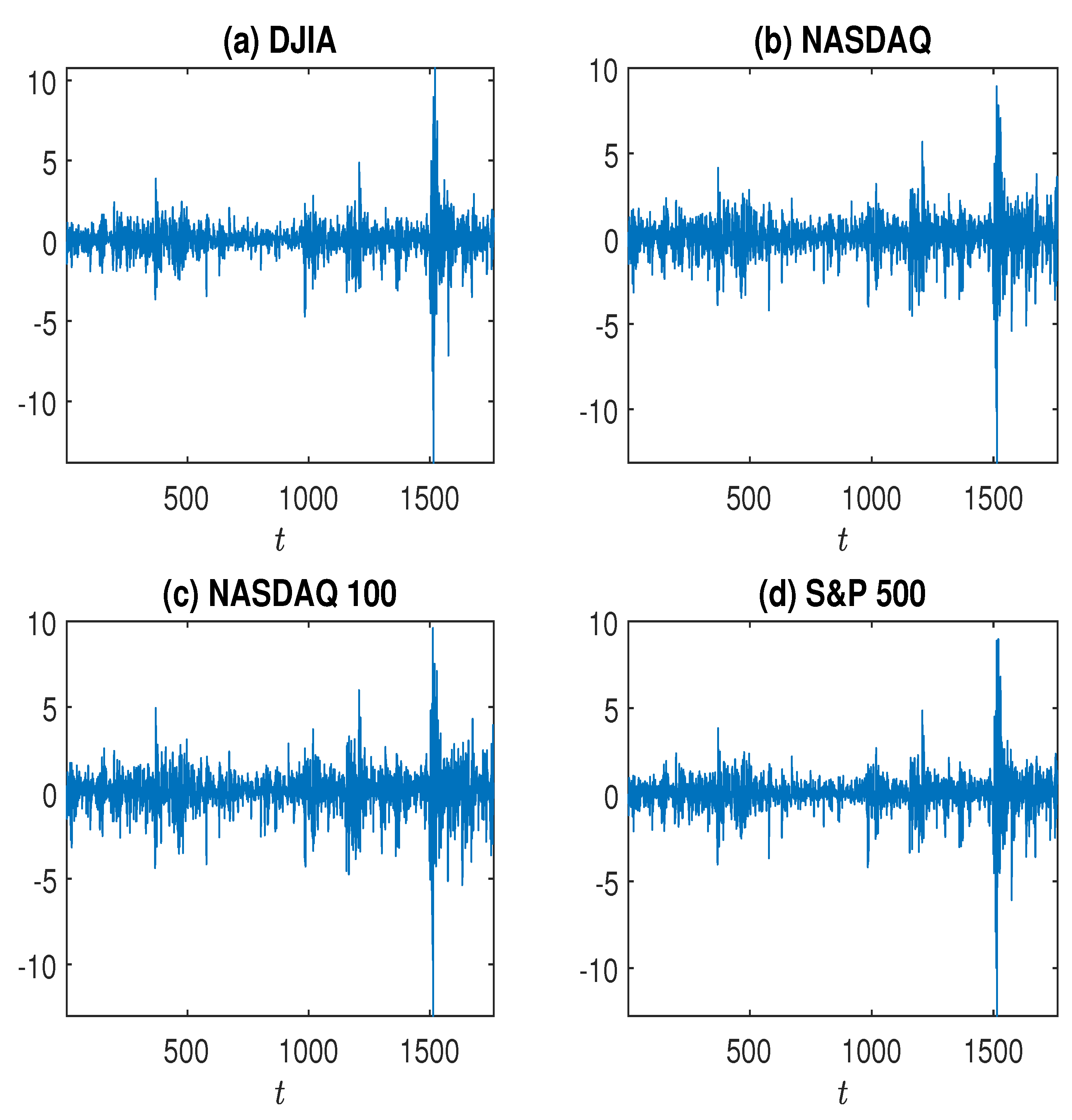
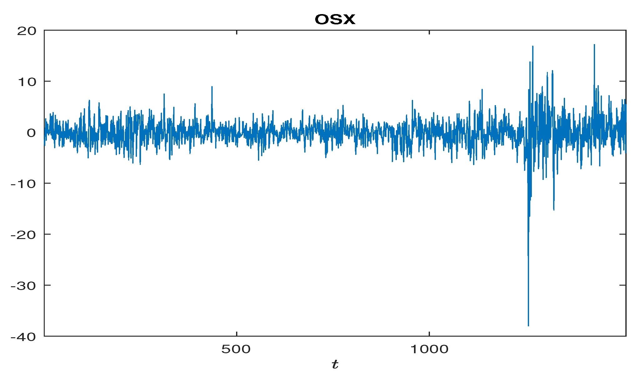
5. Real Examples
6. Concluding Remarks
Author Contributions
Funding
Institutional Review Board Statement
Informed Consent Statement
Data Availability Statement
Acknowledgments
Conflicts of Interest
Appendix A. Proofs
References
- An, Jaehyung, Alexey Mikhaylov, and Sang-Uk Jung. 2021. A linear programming approach for robust network revenue management in the airline industry. Journal of Air Transport Management 91: 101979. [Google Scholar] [CrossRef]
- An, Jaehyung, and Alexey Mikhaylov. 2020. Russian energy projects in South Africa. Journal of Energy in Southern Africa 31: 58–64. [Google Scholar] [CrossRef]
- Amemiya, Takeshi. 1985. Advanced Econometrics. Cambridge: Harvard University Press. [Google Scholar]
- Basrak, Bojan, Richard A. Davis, and Thomas Mikosch. 2002. Regular variation of GARCH processes. Stochastic Processes and Their Applications 99: 95–115. [Google Scholar] [CrossRef] [Green Version]
- Berkes, István, Lajos Horváth, and Piotr Kokoszka. 2003. GARCH processes: Structure and estimation. Bernoulli 9: 201–7. [Google Scholar] [CrossRef]
- Bollerslev, Tim. 1986. Generalized autoregressive conditional heteroskedasticity. Journal of Econometrics 31: 307–27. [Google Scholar] [CrossRef] [Green Version]
- Davis, Richard A., and Thomas Mikosch. 1998. The sample autocorrelations of heavy-tailed processs with applications to ARCH. Annals of Statistics 26: 2049–80. [Google Scholar] [CrossRef]
- Drost, Feike C., and Chris A. J. Klaassen. 1997. Efficient estimation in semiparametric GARCH models. Journal of Econometrics 81: 193–221. [Google Scholar] [CrossRef] [Green Version]
- Drost, Feike C., Chris A. J. Klaassen, and Bas J. M. Werker. 1997. Adaptive estimation in time series models. Annals of Statistics 25: 786–817. [Google Scholar] [CrossRef]
- Engle, Robert F. 1982. Autoregressive conditional heteroskedasticity with estimates of variance of U.K. inflation. Econometrica 50: 987–1008. [Google Scholar] [CrossRef]
- Francq, Christian, and Jean-Michel Zakoïan. 2004. Maximum likelihood estimation of pure GARCH and ARMA-GARCH processes. Bernoulli 10: 605–637. [Google Scholar] [CrossRef]
- Hall, Peter, and Qiwei Yao. 2003. Inference in ARCH and GARCH models. Eonometrica 71: 285–317. [Google Scholar] [CrossRef] [Green Version]
- He, Changli, and Timo Teräsvirta. 1999. Properties of moments of a family of GARCH processes. Journal of Econometrics 92: 173–92. [Google Scholar] [CrossRef]
- He, Yi, Yanxi Hou, Liang Peng, and Jiliang Sheng. 2019. Statistical inference for a relative risk measure. Journal of Business & Economic Statistics 37: 301–11. [Google Scholar]
- Hill, Jonathan B. 2010. On tail index estimation for dependent, heterogeneous data. Econometric Theory 26: 1398–436. [Google Scholar] [CrossRef] [Green Version]
- Johansen, Søren. 1995. Likelihood-based Inference in Cointegrated Vector Autoregressive Models. Oxford: OUP Oxford. [Google Scholar]
- Lange, Theis. 2011. Tail behavior and OLS estimation in AR-GARCH models. Statistica Sinica 21: 1191–200. [Google Scholar] [CrossRef] [Green Version]
- Ling, Shiqing. 1999. On the stationarity and the existence of moments of conditional heteroskedastic ARMA models. Statistica Sinica 9: 1119–30. [Google Scholar]
- Ling, Shiqing. 2003. Adaptive estimators and tests of stationary and non-stationary short and long memory ARIMA-GARCH models. Journal of the American Statistical Association 98: 955–67. [Google Scholar] [CrossRef]
- Ling, Shiqing. 2005. Self-weighted LAD estimation for infinite variance autoregressive models. Journal of the Royal Statistical Society: Series B 67: 381–93. [Google Scholar] [CrossRef]
- Ling, Shiqing. 2007. Self-weighted and local quasi-maximum likelihood estimator for ARMA-GARCH/IGARCH models. Journal of Econometrics 140: 849–73. [Google Scholar] [CrossRef]
- Ling, Shiqing, and Michael McAleer. 2002. Necessary and sufficient moment conditions for the GARCH(r, s) and asymmetric power GARCH(r, s) models. Econometric Theory 18: 722–29. [Google Scholar] [CrossRef] [Green Version]
- Ling, Shiqing, and Wai Keung Li. 1997. Fractional autoregressive integrated moving-average time series with conditional heteroskedasticity. Journal of the American Statistical Association 92: 1184–94. [Google Scholar] [CrossRef]
- Ling, Shiqing, and Michael McAleer. 2003a. Asymptotic theory for a new vector ARMA-GARCH model. Econometric Theory 19: 280–310. [Google Scholar] [CrossRef] [Green Version]
- Ling, Shiqing, and Michael McAleer. 2003b. On adaptive estimation in nonstationary ARMA models with GARCH errors. Annals of Statistics 31: 642–74. [Google Scholar] [CrossRef]
- Pantula, Sastry G. 1989. Estimation of autoregressive models with ARCH errors. Sankhyā: The Indian Journal of Statistics, Series B 50: 119–38. [Google Scholar]
- Setiawan, Budi, Marwa Ben Abdallah, Maria Fekete-Farkas, Robert Jeyakumar Nathan, and Zoltan Zeman. 2021. GARCH (1, 1) models and analysis of stock market turmoil during COVID-19 outbreak in an emerging and developed economy. Journal of Risk and Financial Management 14: 576. [Google Scholar] [CrossRef]
- Weiss, Andrew A. 1986. Asymptotic theory for ARCH models: Estimation and testing. Econometrics Theory 2: 107–31. [Google Scholar] [CrossRef] [Green Version]
- Zhang, G. Peter. 2003. Time series forecasting using a hybrid ARIMA and neural network model. Neurocomputing 50: 159–75. [Google Scholar] [CrossRef]
- Zhang, Rongmao, and Shiqing Ling. 2015. Asymptotic inference for AR models with heavy-tailed G-GARCH noises. Econometric Theory 31: 880–90. [Google Scholar] [CrossRef]
- Zhang, Wenjun, and Jin E. Zhang. 2020. GARCH option pricing models and the variance risk premium. Journal of Risk and Financial Management 13: 51. [Google Scholar] [CrossRef] [Green Version]
- Zhu, Ke, and Shiqing Ling. 2011. Global self-weighted and local quasi-maximum exponential likelihood estimators for ARMA-GARCH/ IGARCH models. Annals of Statistics 39: 2131–63. [Google Scholar] [CrossRef]
- Zhu, Ke, and Shiqing Ling. 2015. LADE-based inference for ARMA models with unspecified and heavy-tailed heteroscedastic noises. Journal of the American Statistical Association 110: 784–94. [Google Scholar] [CrossRef] [Green Version]


| n | |||||||
| 1000 | Bias | −0.0012 | 0.0032 | 0.0189 | 0.0012 | −0.0235 | |
| SD | 0.0443 | 0.0423 | 0.0650 | 0.0278 | 0.0839 | ||
| AD | 0.0424 | 0.0402 | 0.0524 | 0.0290 | 0.0726 | ||
| 2000 | Bias | −0.0017 | 0.0015 | 0.0083 | −0.0000 | −0.0103 | |
| SD | 0.0300 | 0.0293 | 0.0342 | 0.0204 | 0.0471 | ||
| AD | 0.0300 | 0.0285 | 0.0332 | 0.0201 | 0.0469 | ||
| 1000 | Bias | −0.0010 | 0.0022 | 0.0172 | 0.0015 | −0.0210 | |
| SD | 0.0425 | 0.0406 | 0.0657 | 0.0282 | 0.0845 | ||
| AD | 0.0405 | 0.0380 | 0.0526 | 0.0291 | 0.0729 | ||
| 2000 | Bias | −0.0016 | 0.0012 | 0.0073 | −0.0000 | −0.0087 | |
| SD | 0.0283 | 0.0274 | 0.0340 | 0.0205 | 0.0470 | ||
| AD | 0.0286 | 0.0270 | 0.0332 | 0.0202 | 0.0469 | ||
| 1000 | Bias | −0.0032 | 0.0035 | 0.0241 | 0.0020 | −0.0304 | |
| SD | 0.0454 | 0.0414 | 0.0806 | 0.0381 | 0.1079 | ||
| AD | 0.0456 | 0.0433 | 0.0639 | 0.0385 | 0.0909 | ||
| 2000 | Bias | −0.0001 | 0.0014 | 0.0116 | 0.0016 | −0.0148 | |
| SD | 0.0328 | 0.0307 | 0.0426 | 0.0268 | 0.0599 | ||
| AD | 0.0323 | 0.0307 | 0.0397 | 0.0269 | 0.0577 | ||
| 1000 | Bias | −0.0027 | 0.0028 | 0.0237 | 0.0028 | −0.0296 | |
| SD | 0.0444 | 0.0402 | 0.0918 | 0.0390 | 0.1183 | ||
| AD | 0.0443 | 0.0416 | 0.0641 | 0.0387 | 0.0913 | ||
| 2000 | Bias | −0.0008 | 0.0013 | 0.0109 | 0.0019 | −0.0138 | |
| SD | 0.0316 | 0.0296 | 0.0424 | 0.0270 | 0.0598 | ||
| AD | 0.0313 | 0.0295 | 0.0397 | 0.0270 | 0.0578 | ||
| 1000 | Bias | −0.0012 | 0.0016 | 0.0300 | 0.0046 | −0.0395 | |
| SD | 0.0460 | 0.0445 | 0.0867 | 0.0432 | 0.1137 | ||
| AD | 0.0454 | 0.0431 | 0.0734 | 0.0443 | 0.1038 | ||
| 2000 | Bias | 0.0014 | 0.0005 | 0.0126 | 0.0025 | −0.0164 | |
| SD | 0.0312 | 0.0305 | 0.0463 | 0.0325 | 0.0657 | ||
| AD | 0.0323 | 0.0308 | 0.0459 | 0.0316 | 0.0666 | ||
| 1000 | Bias | −0.0022 | 0.0018 | 0.0291 | 0.0054 | −0.0381 | |
| SD | 0.0472 | 0.0448 | 0.0897 | 0.0444 | 0.1166 | ||
| AD | 0.0443 | 0.0417 | 0.0737 | 0.0445 | 0.1042 | ||
| 2000 | Bias | 0.0006 | 0.0007 | 0.0119 | 0.0030 | −0.0155 | |
| SD | 0.0317 | 0.0296 | 0.0462 | 0.0330 | 0.0656 | ||
| AD | 0.0315 | 0.0297 | 0.0459 | 0.0317 | 0.0667 | ||
| n | |||||||||
| 1000 | Bias | 0.0001 | 0.0012 | −0.0034 | 0.0024 | −0.0033 | 0.0015 | ||
| SD | 0.0441 | 0.0412 | 0.0482 | 0.0473 | 0.0518 | 0.0487 | |||
| AD | 0.0437 | 0.0411 | 0.0507 | 0.0474 | 0.0525 | 0.0490 | |||
| 2000 | Bias | −0.0018 | 0.0015 | −0.0009 | 0.0011 | −0.0008 | 0.0010 | ||
| SD | 0.0307 | 0.0299 | 0.0350 | 0.0325 | 0.0382 | 0.0349 | |||
| AD | 0.0311 | 0.0293 | 0.0367 | 0.0344 | 0.0382 | 0.0358 | |||
Publisher’s Note: MDPI stays neutral with regard to jurisdictional claims in published maps and institutional affiliations. |
© 2022 by the authors. Licensee MDPI, Basel, Switzerland. This article is an open access article distributed under the terms and conditions of the Creative Commons Attribution (CC BY) license (https://creativecommons.org/licenses/by/4.0/).
Share and Cite
Ling, S.; Zhu, K. Self-Weighted LSE and Residual-Based QMLE of ARMA-GARCH Models. J. Risk Financial Manag. 2022, 15, 90. https://doi.org/10.3390/jrfm15020090
Ling S, Zhu K. Self-Weighted LSE and Residual-Based QMLE of ARMA-GARCH Models. Journal of Risk and Financial Management. 2022; 15(2):90. https://doi.org/10.3390/jrfm15020090
Chicago/Turabian StyleLing, Shiqing, and Ke Zhu. 2022. "Self-Weighted LSE and Residual-Based QMLE of ARMA-GARCH Models" Journal of Risk and Financial Management 15, no. 2: 90. https://doi.org/10.3390/jrfm15020090
APA StyleLing, S., & Zhu, K. (2022). Self-Weighted LSE and Residual-Based QMLE of ARMA-GARCH Models. Journal of Risk and Financial Management, 15(2), 90. https://doi.org/10.3390/jrfm15020090