Statistical Analysis Dow Jones Stock Index—Cumulative Return Gap and Finite Difference Method

Abstract

This study was motivated by the poor performance of the current models used in stock return forecasting and aimed to improve the accuracy of the existing models in forecasting future stock returns. The current literature largely assumes that the residual term used in the existing model is white noise and, as such, has no valuable information. We exploit the valuable information contained in the residuals of the models in the context of cumulative return and construct a new cumulative return gap (CRG) model to overcome the weaknesses of the traditional cumulative abnormal returns (CAR) and buy-and-hold abnormal returns (BHAR) models. To deal with the residual items of the prediction model and improving the prediction accuracy, we also lead the finite difference (FD) method into the autoregressive (AR) model and autoregressive distributed lag (ARDL) model. The empirical results of the study show that the cumulative return (CR) model is better than the simple return model for stock return prediction. We found that the CRG model can improve prediction accuracy, the term of the residuals from the autoregressive analysis is very important in stock return prediction, and the FD model can improve prediction accuracy.

1. Introduction

The success of investment strategies lies in accurately forecasting the future returns of each of the stocks in the markets place. Analysts have been analyzing all available data and trends in an attempt to identify mispriced securities in order to make profits that are in excess of the profits based on the riskiness of the assets. Practitioners and analysts in this instance believe that markets are not informationally efficient, and that they are able to analyze available data so as to make superior profits. Participants have used the concepts of abnormal return and cumulative abnormal return (CAR) to identify whether the stock prices will rise or decline immediately following some trading activities or events.

Studies by Barber and Lyon (1997), Ziobrowski et al. (2004), Zamanian et al. (2013), Lamba and Tripathi (2015), Mitesh et al. (2016), Campbell et al. (2021), and Hillegeist and Weng (2021) test the impact of trading activities and events on stock prices based on the buy-and-hold abnormal return (BHAR) or the cumulative abnormal return (CAR) models. More efficient stock prices benefit shareholders by reducing information imbalance and improving liquidity. However, there are two main disadvantages for the BHAR model. Firstly, the formula of the BHAR model cannot present a consistent forecasting result with a zero abnormal return at the end of the time period. Based on the BHAR formula $BHA{R}_t={{\displaystyle \prod }}_{t=1}^t(r_t-E(r_t))$, if the terminal value $r_T-E(r_T)\ne 0$, then $\underset{t\to T}{\lim }BHA{R}_t=r_1{r}_2\dots r_{t-1}(r_T-E(r_T))\ne 0$. Secondly, there is a compounding effect suggested by the BHAR model, but the expectation of $E(r_t)$ is a geometric average return, or not a compound average return.

This study aims to overcome the weaknesses of the BHAR model by developing a new model referred to as the cumulative return gap (CRG) model. Moreover, we use the cumulative return gap (CRG) model as an improvement of the CAR and BHAR models to predict stock returns by the autoregressive distributed lag (ARDL) model1. The new CRG model will present a consistent forecasting result with a zero abnormal return at the end of the time period for a cumulative average compound return: $\underset{t\to T}{\lim }{r}_t^{(c,gap)}=\underset{t\to T}{\lim }\left\{{{\displaystyle \prod }}_{t=1}^t{r}_t-{({{\displaystyle \prod }}_{t=1}^t{r}_t)}^{t/T}\right\}$. The empirical study shows that the cumulative return gap is better than the simple abnormal return model for stock return prediction.

A very important role of index forecasting is analyzing time series and building a proper forecasting model. Gijon et al. (2021) focus on how traffic forecasting in telecommunication networks can be treated as a time series analysis problem. Linear time series models, such as autoregressive integrated moving average models, capture trend and short-range dependencies in traffic demand. Studies by Lin et al. (2021) consider interval-valued series data, the analysis of which is conducted in an auto-interval-regressive model using statistics from normal distribution. Similarly, Maratkhan et al. (2021) propose a three-step model on the framework on financial time series to take advantage of the powerful models offered for image classification. However, they all overlooked the residual part of the selected autoregression mode and many researchers have preferred to assume that the residual part is zero (e.g., Devi et al. 2013; Ye and Wei 2015; Zaham and Kenett 2013). However, the residual item generally includes a lot of information, and it is easy to reduce the accuracy of forecasting results when the residual is assumed to be zero. As a result, the key to improving the forecasting accuracy by using autoregressive-related models2 is to forecast the trend of residual items. For this reason, we will analyze the residual part by the normalized probability cumulative distribution function (CDF) and finite difference (FD) methods. Moreover, we will carry out a comparison between residual = 0 and residual ≠ 0 to detect the importance of the residual in stock return forecasting.

2. Literature Review

According to the efficient market hypothesis (EMH), investors and traders in stock markets are not able to make abnormal positive returns by using publicly available information (Hu et al. 2021). However, abnormal phenomena in the financial markets have brought about an impact on classical financial theory. Such assumptions about abnormal positive returns are unrealistic, because people acting to maximize their personal utility in their public capacities as well as their private lives is the most fundamental principle. Ziobrowski et al. (2004) conducted an empirical analysis to test whether U.S. Senators have an informational advantage over other investors in terms of common stock investments by testing for abnormal returns during the period of 1993–1998, proving that stocks purchased by U.S. Senators earn statistically significant positive abnormal returns and outperform the market by 85 basis points per month on a trade-weighted basis. This result proves that U.S. Senators have an informational advantage compared to other investors. Zamanian et al. (2013) used the cumulative abnormal return (CAR) method to test long-run returns from 1 February 2006 to 29 February 2011 on the initial public offerings (IPO) of 18 public and 15 private companies in the Tehran Stock Exchange (TSE), and proved that corporate ownership has no significant impact on the returns of IPOs in the short run or long run. Lamba and Tripathi (2015) used the concepts of average abnormal return (AAR) and cumulative average abnormal return (CAAR) to detect whether Indian firms are able to create value for shareholders after cross-border mergers and acquisitions. Their results proved that acquisitions do not create value to Indian acquiring companies in the long run, and abnormal returns and cumulative abnormal returns have significantly deteriorated since the period of 1998–2009; this value destruction could be attributed to the financial crisis. Bharandev and Rao (2021) examined the stock market and trading volume reaction with respect to the information content of 34 selected companies’ stock splitting announcements between 1 January to 31 July 2016; the average abnormal return (AAR) and cumulative average abnormal return (CAAR) were used to test whether an opportunity was available to make abnormal returns, and their study proved that no one can obtain abnormal returns from the Indian stock market, but stock splitting announcements have a negative impact on stock returns.

Some studies (Ritter 1991; Barber and Lyon 1997; Mohit and Aggarwal 2014; Mitesh et al. 2016) defined two kinds of abnormal return, CAR3 and BHAR4.

The difference between CAR and BHAR is that CAR ignores compounding, but BHAR includes the effect of compounding. Barber and Lyon (1997) proved that the empirical analysis of CAR may result in more bias than BHAR. In fact, there are two disadvantages for buy-and-hold abnormal returns (BHAR), even though they proved that the empirical results of BHAR are much better than CAR. When the variables $r_1,r_2,\dots ,r_t$ are the returns between the time periods of $t\in \left[0,1\right],\left[1,2\right],\dots ,\left[t-1,t\right]$, the expression of ${{\displaystyle \prod }}_{t=1}^t{r}_t$ represents the compounding return of the stock during the time period $t\in \left[0,t\right]$. When we consider the conditional compounding effect, the conditional expected value is $E({{\displaystyle \prod }}_{t=1}^t{r}_t)={{\displaystyle \prod }}_{t=1}^{t-1}{r}_{t}E(r_t)$, then the buy-and-hold abnormal returns will be $BHA{R}_t\left|F_{t-1}=E({{\displaystyle \prod }}_{t=1}^t{r}_t-{{\displaystyle \prod }}_{t=1}^{t}E(r_t))\right|F_{t-1}=r_1{r}_2\dots r_{t-1}E(r_t-E(r_t)|F_{t-1})$. However, if $E(r_T-E(r_T))\ne 0$, there is $\underset{t\to T}{\lim }BHA{R}_t|F_{t-1}=\underset{t\to T}{\lim }\{r_1{r}_2\dots r_{t-1}E(r_t-E(r_t)|F_{t-1})\}\ne 0$, which cannot protect us by obtaining a consistent forecasting result with a zero abnormal return at the end of the time period. Another disadvantage of BHAR is that, theoretically, the expectation of $E(r_t)$ is a geometric average return, but not a compound average return. This is not consistent with the main assumption of the compounding effect suggested by the BHAR model.

To overcome these weaknesses of the traditional cumulative abnormal returns (CAR) and buy-and-hold abnormal returns (BHAR) models, we define a new cumulative return gap (CRG) model. The principal of our cumulative return gap (CRG) model is similar to the concept of buy-and-hold abnormal returns (BHAR).

Assume the time variable is $t\in \left[0,T\right]$, where $T$ is the biggest width of the time window; variable $p_t$ represents the stock price, $p_0=p_1$; the return index $r_t$ is defined as $r_t=p_t/p_{t-1}$, $r_1=1$; the new defined cumulative return index is defined as $r_t^{(c)}={{\displaystyle \prod }}_{t=1}^t{r}_t$, $r_1^{(c)}=r_1=1$; the average compound return of the cumulative return $r_t^{(c)}$ is defined as $r_t^{(ave)}={(r_t^{(c)})}^{\frac{1}{t}}$, $r_T^{(ave)}={(r_T^{(c)})}^{\frac{1}{T}}$; and the average cumulative compound return index of the cumulative return index $r_t^{(c)}$ is defined as $r_t^{(c,ave)}={(r_T^{(ave)})}^t$. Based on these assumed variables, the cumulative return gap (CRG) is defined as

$$r_t^{(c,gap)}=r_t^{(c)}-r_t^{(c,ave)}={\displaystyle \prod }_{t=1}^t{r}_t-{(r_T^{(ave)})}^t={\displaystyle \prod }_{t=1}^t{r}_t-{({(r_T^{(c)})}^{\frac{1}{T}})}^t={\displaystyle \prod }_{t=1}^t{r}_t-{({\displaystyle \prod }_{t=1}^T{r}_t)}^{\frac{t}{T}}$$

When comparing our new concept of the cumulative return gap (CRG) with the concept of buy-and-hold abnormal returns (BHAR), CRG will provide us with a consistent forecasting result with a zero abnormal return at the end of the time period.

$$\underset{t\to T}{\lim }{r}_t^{(c,gap)}=\underset{t\to T}{\lim }\left\{{\displaystyle \prod }_{t=1}^t{r}_t-{({\displaystyle \prod }_{t=1}^t{r}_t)}^{\frac{t}{T}}\right\}=0$$

Furthermore, the average compound return $r_T^{(ave)}={(r_T^{(c)})}^{\frac{1}{T}}$ is a constant during the time period $t\in \left[0,T\right]$, which is also a compound return.

Traditionally, the cumulative abnormal return (CAR) and BHAR models are used to study the long-term behavior of stock returns during a particular period, such as several days, several months, or several years. However, there are fewer studies using the cumulative abnormal return model to forecast stock returns. Our research will fill the research gap by using the cumulative return gap (CRG) model as an improvement of the cumulative abnormal return model to forecast stock returns.

The aim of prediction is to look for future information on the basis of previous information. Based on historical events, prediction is aimed towards forecasting the events which may happen in the future. Shen et al. (2012) believe that a single stock price can be directly predicted by its autocorrelation, because the performance of a stock market prediction heavily depends on the correlation between the data used. If the trend of a stock price is always an extension of yesterday, or if a time series of the stock market price has a high autocorrelation, the accuracy of prediction should be fairly high. The results of Shen et al. (2012) prove that autocorrelation is a very useful tool for predicting a single stock price; however, their analysis does not mention the disturbance of the regression model’s residual noise, which may influence the accuracy of the prediction values.

A very important part of forecasting is analyzing the time series and building a proper forecasting model, especially when the initial stochastic time series of the return is nonstationary in nature and can be analyzed based on the selection of any method (Rabbani et al. 2021). When autoregressive-related models are used to analyze time series, such as in the ES, AR, MA, ARMA, ARIMA and SARMA models, many researchers prefer to assume that the residual item is zero with the absolute lowest error.

Usually, $ARIMA(p,d,q)$, also known as the Box–Jenkins method, is used to remove the trend of the series by differencing so that a stationary series is obtained by transforming a non-stationary series (Dimri et al. 2020). Here, the parameter $p$ represents the order of the autoregressive process, such as a model of $AR(p)$; the parameter $q$ represents the order of the moving average process, such as a model of $MA(q)$; and the parameter $d$ represents the order of differencing of the time series. Samrad et al. (2021) suggest that the ARIMA modelling approach, according to various measures, is the most effective and best model for predicting trend stock prices by keeping the residuals at zero. Zaham and Kenett (2013) also use ARIMA models such as $ARIMA(1,1,1)$ and $ARIMA(2,1,2)$ to forecast the stock prices by letting residuals be zero. Ye and Wei (2015) think that since the ARIMA model is a typical linear time series model, it is not easy to represent the nonlinear dynamic system of stock markets; if the ARIMA model is used to predict complex time series such as stock prices, the forecasting result will be not ideal. Skare et al. (2021) preferred to use the autoregressive model (AR) and the vector autoregressive model (VAR) to perform the purpose of forecasting. The autoregressive model is a good model when the dependent variable is a univariate; however, when the number of dependent variables is more than one, then the vector autoregressive model has an advantage over the former.

The residual item generally includes a lot of private information and some public information such as economic shocks, and it is easy to reduce the accuracy of forecasting when the residual is assumed to be zero, as Dimri et al. (2020) have done. Because the auto-regressive-related models such as SE, AR, MA, ARMA, and ARIMA are based on linear models, most of the nonlinear information is composited into the residual items. If the residual items are simply assumed to be zero, most of the nonlinear information will be removed, and the accuracy of forecasting will be disturbed. Even though the moving average (MA) model considers the influence of residual lagged items, it is based on linear models and not on nonlinear models. If the residual items are mostly not considered, the auto-regressive-related models will not be able to significantly improve the accuracy of forecasting within the models. The key of improving the forecasting accuracy by using auto-regressive-related models is to forecast the trend of residual items. For this reason, we will try to improve the forecasting accuracy by forecasting the residual items. The probability method and finite difference (FD) method will be used to deal with the residual items.

Thus, for this study, we chose the autoregressive distributed lag (ARDL) model as the regression model to predict the underlying stock returns. The ARDL model was first defined by Pesaran and Shin (1999). The purpose of the ARDL model is to represent the long-term relationships between variables in econometric analysis.

The general ARDL(p, q) model can be defined as

$$y_t={\omega }_0+{\omega }_{1}t+{\displaystyle \sum }_{i=1}^p{\alpha }_i{y}_{t-i}+{\beta }_0{x}_t+{\displaystyle \sum }_{j=1}^q{\beta }_i{x}_{t-j}+u_t$$

The ARDL model represents the long-term relationship between the variable $y_t$ and $x_t$, where $x_t$ is the $k (k>1)$ dimensional order 1 difference stationary variable ($I(1)$ for short, meaning it has an order 1 unit root) or an order 0 difference stationary variable ($I(0)$ for short, meaning the level variable is stationary). If the variable $x_t$ is the order 1 difference stationary variable, even though it has an order 1 unit root, the vector autoregressive process in $\Delta x_t$ is stable.

Wang et al. (2021) have approved that the ARDL model is good for dealing with the time series econometric variables; additionally, the ARDL model has the advantage of predicting consistent estimates of the long-run coefficients and cointegrating relationships between variables that are asymptotically normal but irrespective of whether the underlying stock prices’ regressions are I(1) or I(0).

Li et al. (2020) preferred to use the autoregressive distributed lag (ARDL) model proposed by Shin et al. (2014) for prediction, because the ARDL model has three important stages that include changes in the policy rate: first, it can be applied regardless of what levels of stationary or what orders of unit root the underlying variables; second, ARDL is suitable for both big and small samples; and third, the appropriate order modification of ARDL is sufficient for simultaneously correcting the residual serial correlation and the problem of endogenous variables. In this paper, the prediction model for the cumulative return index $r_t^{(c)}$ will be defined by the following ARDL-CRG model

$$r_t^{(c)}=k_0+k_1{r}_t^{(c,ave)}+\beta \ln t+{\displaystyle \sum }_{i=1}^p{\alpha }_i{r}_{t-i}^{(c,gap)}+a_t$$

For carrying out a comparison, the AR model is also usually used to build the prediction model

$$r_t={\alpha }_0+{\alpha }_1{r}_{t-1}+\cdots +{\alpha }_p{r}_{t-p}+a_t$$

For both the ARDL and AR models, because the residual item $a_t$ is very important for building prediction models, we will borrow the finite difference method to deal with the residual item $a_t$. For dealing with the residual variable $a_t$, we will focus on dealing with the probability variable $q_t$. The relationship between $a_t$ and $q_t$ is

$$a_t=-\ln (\frac{1}{q_t}-1)\mathrm{or}{q}_t=\frac{1}{1+e^{-a_t}}$$

There are seldom studies that use the finite difference method to deal with the residual items of $a_t$. We will apply different orders of the finite difference to the probability variable $q_t$.

3. Methodology and Data

3.1. Data

A daily closing price index of the Dow Jones Industry Index is used as the time series samples (Ranco et al. 2015; Stekelenburg et al. 2015). The time intervals are listed within the period of 1 April 2010 to 8 July 2016.5 The total transaction days, or the observations, are 1531 days. The daily closing price index is simply gathered from the calendar dates when the US stock markets were open. Very few data were canceled if the data were from a special holiday when the US stock markets were not open. All of the calculations in this paper will be conducted using EViews 8.0 statistical software. The variable $r_t$ is defined as a daily closing return index of the Dow Jones Industry Index.

Table 1. Main variables for building the four kinds of models: AR-FD, AR-GARCH-FD, ARDL-CRG-FD and ARDL-CRG-GARCH-FD.

Variables	Explanations	Models	Variables	Explanations
$p_t$	Price of an asset	AR	$r_{a,t}$	Return index of an asset
$r_t$	Return index of an asset	AR	${\mu }_{a,t}$	$\mathrm{Expected}\mathrm{value}\mathrm{of}{r}_{a,t}$
$r_t^{(c)}$	Cumulative compound return index	AR	$a_t$	Residual item of AR model
$r_T^{(c)}$	Cumulative compound return index	AR-FD	$q_t^{(a)}$	$\mathrm{Cumulative}\mathrm{probability}\mathrm{of}\mathrm{quantile}{a}_t$
$r_T^{(ave)}$	Average cumulative compound return	AR-FD	$r_{a,t}^{(2)}$	Return from the 2nd-order difference
$r_t^{(c,ave)}$	Cumulative average compound return	AR-FD	$r_{a,t}^{(3)}$	Return from the 3rd-order difference
$r_t^{(c,gap)}$	Cumulative return gap (CRG)	AR-FD	$r_{a,t}^{(4)}$	Return from the 4th-order difference
$q_t^{(a)}$	$\mathrm{Cumulative}\mathrm{probability}\mathrm{of}\mathrm{quantile}{a}_t$	AR-FD	$r_{a,t|j=p}$	$\mathrm{Predictions}\mathrm{of}{r}_{a,t}$$\mathrm{when}{q}_{t-p}^{(a)}$ used
$d^n{q}_t^{(a)}$	$\mathrm{nth}-\mathrm{order}\mathrm{finite}\mathrm{difference}\mathrm{of}{q}_t^{(a)}$	AR-GARCH-FD	$q_{a,t}^{(e)}$	$\mathrm{Cumulative}\mathrm{probability}\mathrm{of}\mathrm{quantile}{e}_{a,t}$
$d^2{q}_t^{(a)}$	2nd-order finite difference of $q_t^{(a)}$	AR-GARCH-FD	$r_{a,t}^{(e)}$	$\mathrm{Predictions}\mathrm{of}{r}_{a,t}$$\mathrm{when}{q}_{a,t}^{(e)}$ used
$d^3{q}_t^{(a)}$	3rd-order finite difference of $q_t^{(a)}$	AR-GARCH-FD	$r_{a,t|j=p}^{(e)}$	$\mathrm{Predictions}\mathrm{of}{r}_{a,t}$$\mathrm{when}{q}_{t-p}^{(a)}$ used
$d^4{q}_t^{(a)}$	4th-order finite difference of $q_t^{(a)}$	ARDL-CRG	$r_{b,t}^{(c)}$	$\mathrm{Prediction}\mathrm{value}\mathrm{of}{r}_t^{(c)}$
$a_t$	Residual item of a regression model	ARDL-CRG	${\mu }_{b,t}^{(c)}$	$\mathrm{Expected}\mathrm{value}\mathrm{of}{r}_t^{(c)}$
$q_t$	$\mathrm{Cumulative}\mathrm{probability}\mathrm{of}\mathrm{quantile}{a}_t$	ARDL-CRG	$b_t$	Residual of the ARDL-CRG model
${\sigma }_t$	$\mathrm{Dynamic}\mathrm{volatility}\mathrm{based}\mathrm{on}{a}_t$	ARDL-CRG-FD	$q_t^{(b)}$	$\mathrm{Cumulative}\mathrm{probability}\mathrm{of}\mathrm{quantile}{b}_t$
${\epsilon }_t$	$\mathrm{Standardized}\mathrm{error}\mathrm{item}\mathrm{from}{a}_t/{\sigma }_t$	ARDL-CRG-FD	$r_{b,t}^{(2)}$	Return from the 2nd-order difference
$e_t$	$\mathrm{Standardized}\mathrm{error}\mathrm{item}\mathrm{from}{\epsilon }_t$	ARDL-CRG-FD	$r_{b,t}^{(3)}$	Return from the 3rd-order difference
${\sigma }_{a,t}$	$\mathrm{Dynamic}\mathrm{volatility}\mathrm{based}\mathrm{on}{a}_t$	ARDL-CRG-FD	$r_{b,t}^{(4)}$	Return from the 4th-order difference
${\epsilon }_{a,t}$	$\mathrm{Standardized}\mathrm{error}\mathrm{item}\mathrm{from}{a}_t/{\sigma }_{a,t}$	ARDL-CRG-FD	${\mu }_{b,t}$	$\mathrm{Expected}\mathrm{value}\mathrm{of}{r}_t$
$e_{a,t}$	$\mathrm{Standardized}\mathrm{error}\mathrm{item}\mathrm{from}{\epsilon }_{a,t}$	ARDL-CRG-FD	$r_{b,t|j=p}$	$\mathrm{Predictions}\mathrm{of}{r}_{b,t}$$\mathrm{when}{q}_{t-p}^{(b)}$ used
${\sigma }_{b,t}$	$\mathrm{Dynamic}\mathrm{volatility}\mathrm{based}\mathrm{on}{b}_t$	ARDL-CRG-GARCH-FD	$q_{b,t}^{(e)}$	$\mathrm{Cumulative}\mathrm{probability}\mathrm{of}\mathrm{quantile}{e}_{b,t}$
${\epsilon }_{b,t}$	$\mathrm{Standardized}\mathrm{error}\mathrm{item}\mathrm{from}{b}_t/{\sigma }_{b,t}$	ARDL-CRG-GARCH-FD	$r_{b,t}^{(e)}$	$\mathrm{Predictions}\mathrm{of}{r}_{b,t}$$\mathrm{when}{q}_{b,t}^{(e)}$ used
$e_{b,t}$	$\mathrm{Standardized}\mathrm{error}\mathrm{item}\mathrm{from}{\epsilon }_{b,t}$	ARDL-CRG-GARCH-FD	$r_{b,t|j=p}^{(e)}$	$\mathrm{Predictions}\mathrm{of}{r}_{b,t}$$\mathrm{when}{q}_{b,t-p}^{(e)}$ used

shows the main variables used in this paper. Variables will be explained in detail when they are introduced in this paper.

3.2. Cumulative Return

Based on the definition of a one-period simple return, the time-varying variable $r_t$ can represent the simple return for a holding asset from the time interval $\left[t-1,t\right]$ (Tsay 2005).

When the time interval is defined as $t\in \left[0,t\right]$, the cumulative return index $r_t^{(c)}$ of an underling stock can be rewritten as6

$$r_t^{(c)}=\{\begin{array}{cc}{r}_{t-1}^{(c)}{r}_t,& t=1,2,\dots ,T\\ 1& t=0\end{array}\mathrm{where}{r}_t=\{\begin{array}{cc}\frac{p_t}{p_{t-1}},& t=1,2,\dots ,T\\ 1& t=0\end{array}$$

(1)

Then, for representing the gross return between a long time interval $\left[0,t\right]$, there is a relationship between the cumulative return $r_t^{(c)}$ and the simple return $r_t,$ which can be written as

$$r_t^{(c)}=r_t{r}_{t-1}\dots r_2{r}_1$$

(2)

The time variable $T$ is the terminal point of the time period. When the simple return $r_t$ is based on the time interval $t\in \left[t-1,t\right]$, the cumulative return $r_t^{(c)}$ is based on the time interval $t\in \left[0,t\right]$.

3.3. Cumulative Average Compound Return and the Cumulative Return Gap

The principle of this study is to use the predicted value of the cumulative return $r_t^{(c)}$ to obtain the forecasting value of a simple return $r_t$ by Formula (2). Thus, we need a deeper understanding of $r_t^{(c)}$ for several parts. For this paper, we define two new factors $r_t^{(c,ave)}$ and $r_t^{(c,gap)}$, which represent the cumulative average compound return (CACR) and the cumulative return gap (CRG), respectively.

If $t=T$ is the final value of the cumulative return $r_t^{(c)}$, then $r_T^{(ave)}$ can represent the average change of $r_t^{(c)}$ in a constant compound average rate

$$r_t^{(ave)}={(r_t^{(c)})}^{\frac{1}{t}}, t=1,2,\dots ,T$$

(3)

As a result, the cumulative average compound return (CACR) will be defined as

$$r_t^{(c,ave)}={(r_T^{(ave)})}^t={(r_T^{(c)})}^{\frac{t}{T}}, t=1,2,\dots ,T$$

(4)

where the curve of the cumulative return index $r_t^{(c)}$ will move around the curve of the cumulative average compound return index $r_t^{(c,ave)}$.

Then, the gap between the cumulative return $r_t^{(c)}$ and the cumulative average compound return $r_t^{(c,ave)}$ can be represented as $r_t^{(c,gap)}$

$$r_t^{(c,gap)}=r_t^{(c)}-r_t^{(c,ave)}, t=1,2,\dots ,T$$

(5)

The variable $r_t^{(c,gap)}$ represents the cumulative return gap, which can be seen as a cumulative risk premium of a risk asset. The curve of the cumulative return gap index $r_t^{(c,gap)}$ will move around the horizontal line. After carrying out the replacement of $r_t^{(c)}-r_t^{(c,ave)}$, the characteristics of the cumulative risk premium $r_t^{(c,gap)}$ during a long term period of $t\in \left[0,t\right]$ are as similar as the characteristics of the risk premium $r_t-r_f$ in the CAPM model during a short-term period of $t\in \left[t-1,t\right]$.7

3.4. ARDL-CRG Model

The first prediction model for this paper is to transfer the residual term of the ARDL regression model from a quantile to a probability. Once we have the factors of $r_t^{(c,ave)}$ and $r_t^{(c,gap)}$, we can run an ARDL regression model to present the cumulative return $r_t^{(c)}$. Because the cumulative return gap (CRG) is introduced to the ARDL model, this model can be defined as an ARDL-CRG model

$$r_t^{(c)}=k_0+k_1{r}_t^{(c,ave)}+\beta \ln t+{{\displaystyle \sum }}_{i=1}^p{\alpha }_i{r}_{t-i}^{(c,gap)}+a_t\mathrm{where}E(a_t|F_{t-1})=0$$

(6)

Here, the residual variable $a_t$ can be seen as a quantile of a probability variable $q_t$. The probability of the cumulative distribution function (CDF) (Figure 1) can be defined as

$$F(x)=\frac{1}{1+e^{-x}},x\in (-\infty ,+\infty ),\underset{x\to -\infty }{\lim }F(x)=0,\underset{x\to +\infty }{\lim }F(x)=1,F(x)\in (0,1)$$

(7)

When $a_t\in (-\infty ,+\infty )$, assume variable $q_t$ represents the cumulative probability of the residual variable $a_t$, then the probability function is $q_t=F(a_t)$ and $q_t\in (0,1)$, then

$$a_t=-\ln (\frac{1}{q_t}-1)$$

(8)

Thus, the cumulative return prediction model of ARDL-CRG will be rewritten as a new type as follows:

$$r_t^{(c)}=k_0+k_1 r_t^{(c,ave)}+\beta \ln t+{\displaystyle \sum }_{i=1}^p{\alpha }_i r_{t-i}^{(c,gap)}-\ln (\frac{1}{q_t}-1)$$

(9)

It is clear that the ARDL-CRG model has two types: one directly uses the residual item $a_t$, and the other indirectly uses the probability item $q_t$. Both are ARDL-CRG models.

Because the value interval of the function $F(x)$ is $(0,1)$ when $x\in (-\infty ,+\infty )$, it is a cumulative probability function. It is easy to transfer the residual item to a probability item.

3.5. ARDL-CRG-GARCH Model

The second prediction model for this paper is to use the GARCH8 model to present the residual term of ARDL regression. The conditional volatility in the GARCH (1,1) model is defined as

$${\sigma }_t^2=\omega +\alpha a_{t-1}^2+\beta {\sigma }_{t-1}^2, a_t={\sigma }_t{\epsilon }_t, \mathrm{Var}(a_t)={\sigma }_a^2$$

(10)

Theoretically, the random variable ${\epsilon }_t~N(0,1)$ is distributed as a standardized normal distribution. However, because the regressive error is unavoidable, for conducting regressive estimation accurately, assume the random variable ${\epsilon }_t~N({\mu }_0,{\sigma }_0^2)$, then define a standardized random variable $e_t$ as

$$e_t=\frac{{\epsilon }_t-{\mu }_0}{{\sigma }_0}, {\epsilon }_t={\mu }_0+{\sigma }_0{e}_t$$

(11)

Thus, the residual variable $a_t$ can be defined as

$$a_t={\sigma }_t{\epsilon }_t={\sigma }_t({\mu }_0+{\sigma }_0{e}_t),e_t~N(0,1)$$

(12)

Again, we can transfer the standardized residual item $e_t$ to a probability variable $q_t=F(e_t)$, and the inverse relation between them is $e_t=F^{-}(q_t)=-\ln (\frac{1}{q_t}-1)$. If the dynamic volatility variable ${\sigma }_t$ is introduced to the ARDL-CRG model, then we can obtain an ARDL-CRG-GARCH model, which has two types, as follows:

$$r_t^{(c)}=k_0+k_1{r}_t^{(c,ave)}+\beta \ln t+{\displaystyle \sum }_{i=1}^p{\alpha }_i{r}_{t-i}^{(c,gap)}+{\sigma }_t({\mu }_0+{\sigma }_0{e}_t)$$

(13)

$$r_t^{(c)}=k_0+k_1 r_t^{(c,ave)}+\beta \ln t+{\displaystyle \sum }_{i=1}^p{\alpha }_i r_{t-i}^{(c,gap)}+{\sigma }_t({\mu }_0-{\sigma }_0\ln (\frac{1}{q_t}-1))$$

(14)

The ARDL-CRG-GARCH model uses a standardized residual variable $e_t$ to represent the residual of the model, and then transfers this standardized residual variable to a probability variable $q_t$ to represent the residual of the model.

4. Empirical Results

4.1. Return Index

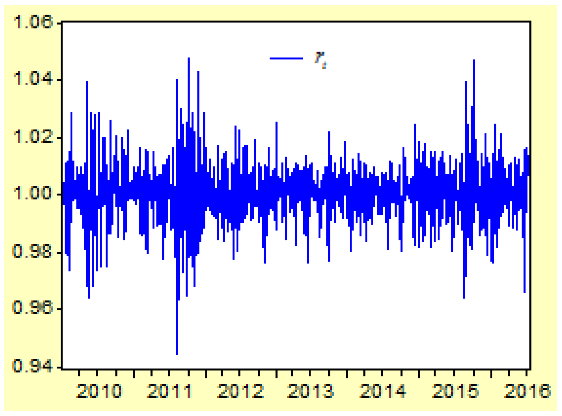
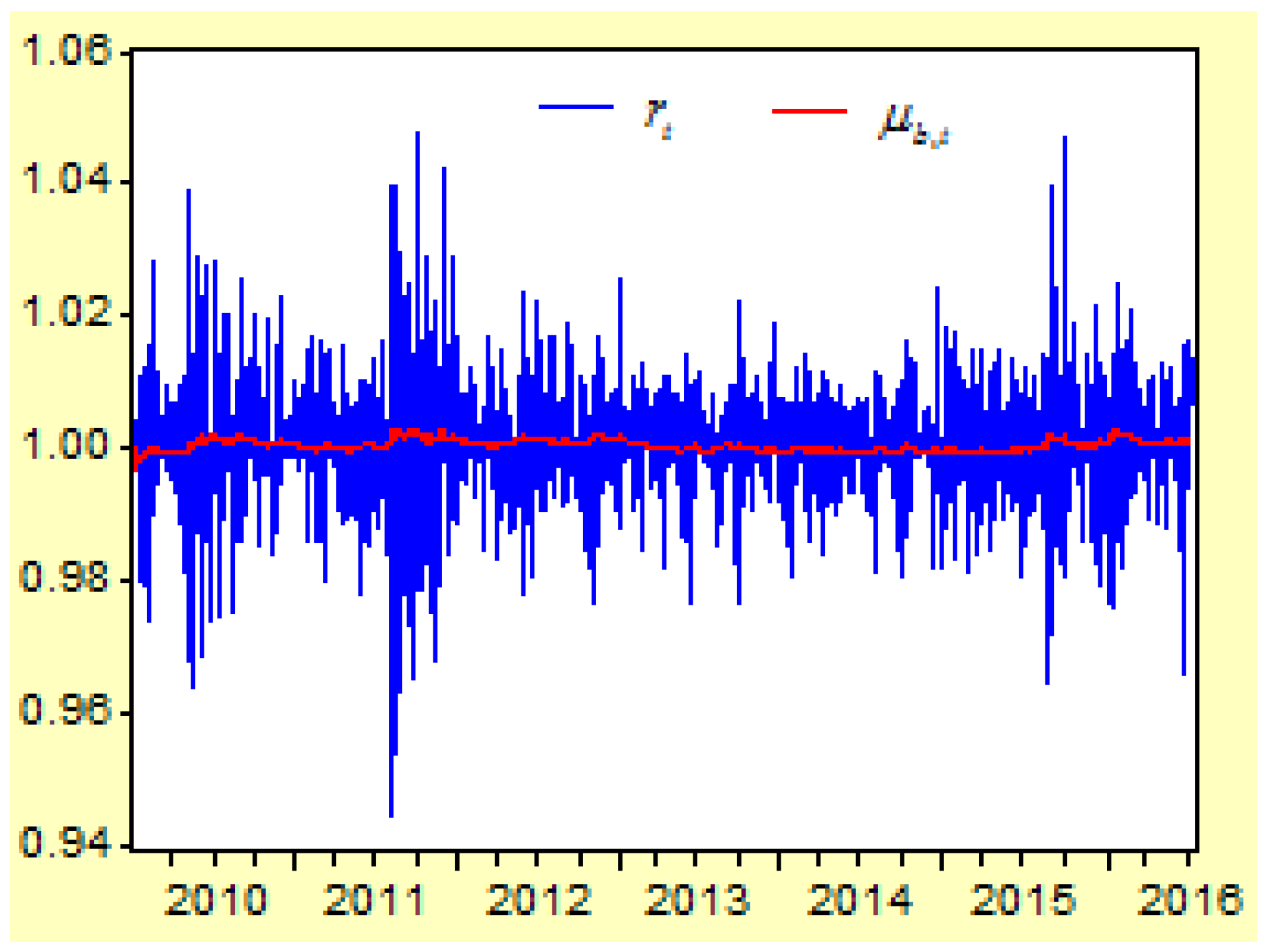
Figure 2 shows the moving curves of the return index $r_t$ of the US Dow Jones Industry Index between 1 April 2010 and 8 July 2016. The sample size is 1531, and the time interval is $t\in \left[0,T\right]$, $T=1531$. There are three cluster vibrations during 2010, 2011, and 2015. These cluster vibrations can be expressed by a GARCH model.

Here we can see that the term of the return index $r_t$ shows the moving trend of a stock price during a short period $t\in \left[t-1,t\right]$. When the return index $r_t$ is defined as $r_t=\frac{p_t}{p_{t-1}}$, it shows that the trend of a stock price is down when $p_t<p_{t-1}$ or up when $p_t>p_{t-1}$. The purpose of forecasting is to predict the moving trend of a stock price in the next time $t$ when the information set $F_{t-1}=\left\{r_1,r_2,\dots ,r_{t-1}\right\}$ is already known.

4.2. Autocorrelation Test for the Return Index

Table 2. Autocorrelation (AC) values and Ljung and Box (1978) statistics and probabilities for time series of the return index.

Variable

AC(1)

Q(1)

P(1)

AC(5)

Q(5)

P(5)

AC(10)

Q(10)

P(10)

AC(15)

Q(15)

P(15)

$r_t$

−0.052

4.1099

0.043

−0.089

31.848

0.000

0.013

32.854

0.000

−0.017

42.504

0.000

Variable

AC(20)

Q(20)

P(20)

AC(25)

Q(25)

P(25)

AC(30)

Q(30)

P(30)

AC(35)

Q(35)

P(35)

$r_t$

−0.040

54.108

0.000

−0.040

58.371

0.000

−0.007

65.140

0.000

0.035

74.216

0.000

lists the test results of the autocorrelations, Ljung and Box (1978) statistics and related probabilities for the return index $r_t$. It shows a significant autocorrelation between $r_t$ and $r_{t-1} (t=1,2,\dots ,t-1)$ at the probability degree levels of 5% and 1%.

These autocorrelations are better expressed in an $AR(p)$ model as $r_t={\alpha }_0+{\alpha }_1{r}_{t-1}+\cdots ++{\alpha }_p{r}_{t-p}+a_t$. Generally, when defined as ${\mu }_t={\alpha }_0+{\alpha }_1{r}_{t-1}+\cdots ++{\alpha }_p{r}_{t-p}$, the $AR(p)$ model will be $r_t={\mu }_t+a_t$. If the information set $F_{t-1}=\left\{r_1,r_2,\dots ,r_{t-1}\right\}$ is already known, then $E(r_t|F_{t-1})={\mu }_t$, $E(a_t|F_{t-1})=0$, $\mathrm{Var}(r_t|F_{t-1})=\mathrm{Var}(r_t|F_{t-1})={\sigma }_t^2$. Here, the expectations and variances are conditional expectations and conditional variances.

For building a stable autoregressive model, it is necessary to test if there are any unit roots for the time series of the return index. By using an ADF unit root test,

Table 3. Autocorrelation (AC) values and Ljung and Box (1978) statistics and probabilities for difference time series of residual probability.

Variable	AC(1)	Q(1)	P(1)	AC(5)	Q(5)	P(5)	AC(10)	Q(10)	P(10)	AC(20)	Q(20)	P(20)
$q_t^{(a)}$	0.001	0.0005	0.982	−0.002	0.0236	1.000	0.009	1.0563	1.000	−0.040	18.650	0.545
$d{q}_t^{(a)}$	−0.500	381.33	0.000	−0.003	381.36	0.000	−0.016	382.37	0.000	−0.022	406.78	0.000
Variable	AC(1)	Q(1)	P(1)	AC(5)	Q(5)	P(5)	AC(10)	Q(10)	P(10)	AC(20)	Q(20)	P(20)
$d^2{q}_t^{(a)}$	−0.667	678.44	0.000	−0.005	721.33	0.000	−0.027	723.33	0.000	−0.017	759.94	0.000
$d^3{q}_t^{(a)}$	−0.750	858.30	0.000	−0.005	1000.9	0.000	−0.033	1004.0	0.000	−0.019	1053.7	0.000
$d^4{q}_t^{(a)}$	−0.800	976.19	0.000	−0.005	1243.9	0.000	−0.039	1248.2	0.000	−0.023	1310.4	0.000

has listed the t-statistic values and probabilities under the three criteria of AIC, SIC and HQC. We can see that there are not any unit roots at the three levels’ time series of level variables, first-order difference variables, and second-order difference variables. Because the return index $r_t$ is an autocorrelation time series, and it does not have any unit roots, we will build an autoregressive model to carry out forecasting tasks. 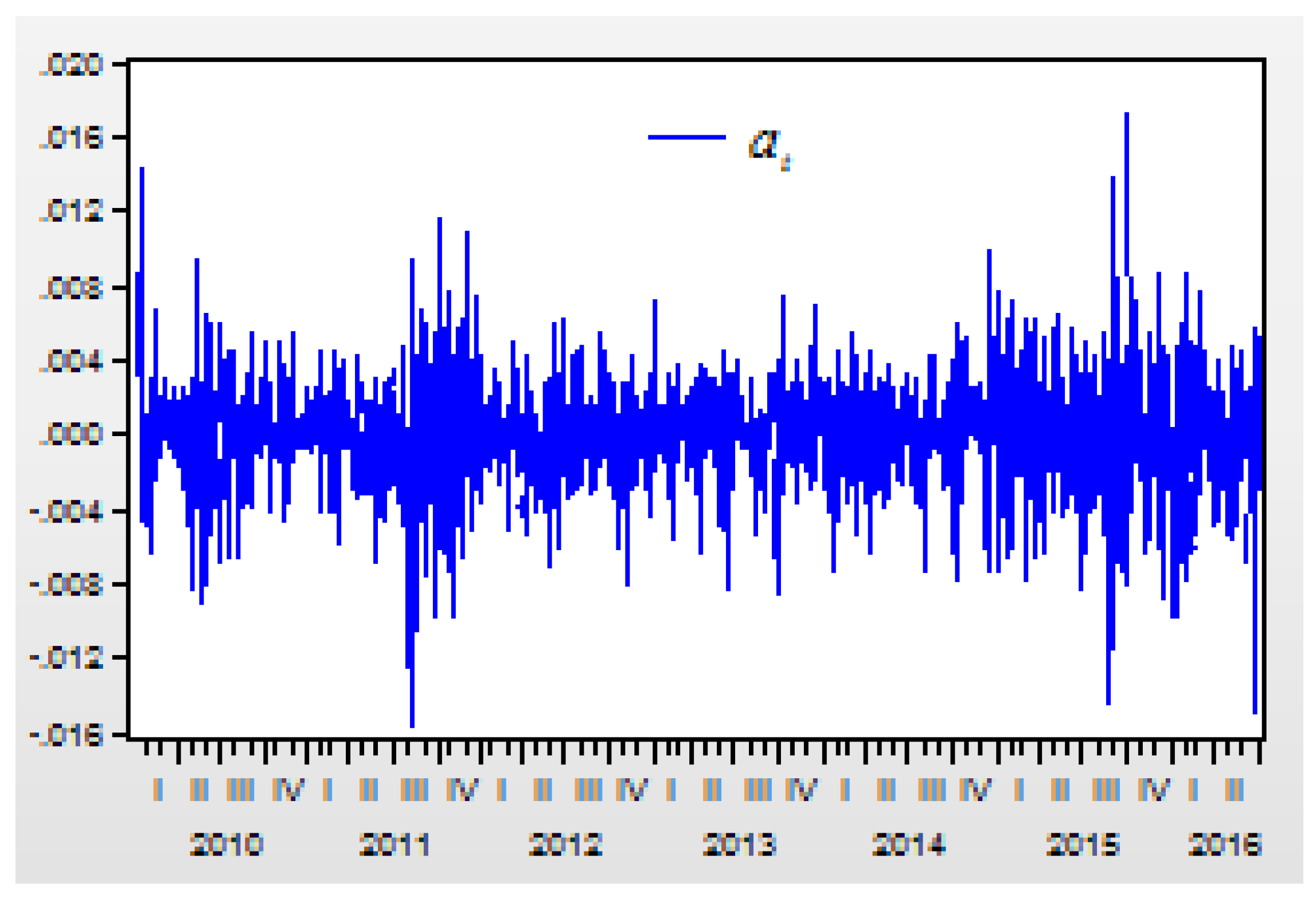Figure 3 shows the residual item $a_t$ from AR model of $r_{a,t}={\mu }_{a,t}+a_t$.

4.3. AR(p) Prediction Model for Return Index

Because the return index $r_t$ is an autocorrelation time series, and it does not have any unit roots, we will build an autoregressive model to carry out forecasting tasks.

After assessing many autoregressive models, next $AR(5)$ model is selected

$$r_{a,t}={\mu }_{a,t}+a_t$$

$${\mu }_{a,t}=1.190795-0.045747r_{t-1}+0.020058r_{t-2}-0.086443r_{t-3}+0.005487r_{t-4}-0.083679r_{t-5}$$

$$R^2=0.0181,S.E.=0.0095,AIC=-6.4626,SIC=-6.4416$$

This $AR(5)$ model has a very small determined coefficient as $R^2=0.0181$. When define $r_{a,t}={\mu }_{a,t}+a_t$, the residual item $a_t$ may include too much information about the return index $r_t$. Figure 3 shows the residual item $a_t$ form AR model of $r_{a,t}={\mu }_{a,t}+a_t$. The correlation between the return index $r_t$ and its residual item $a_t$ of $AR(5)$ model is 0.9908. The correlation is as high as $\mathrm{Corr}(r_t,a_t)0.9908$. For this reason, it is very important to estimate the values of residual items.

4.4. Direct Prediction of the Return Index Based on the Finite Difference Method and the AR-FD Model

For improving the prediction accuracy of the AR model, we will introduce the finite difference (FD) method to the AR model and build a new AR-FD model.

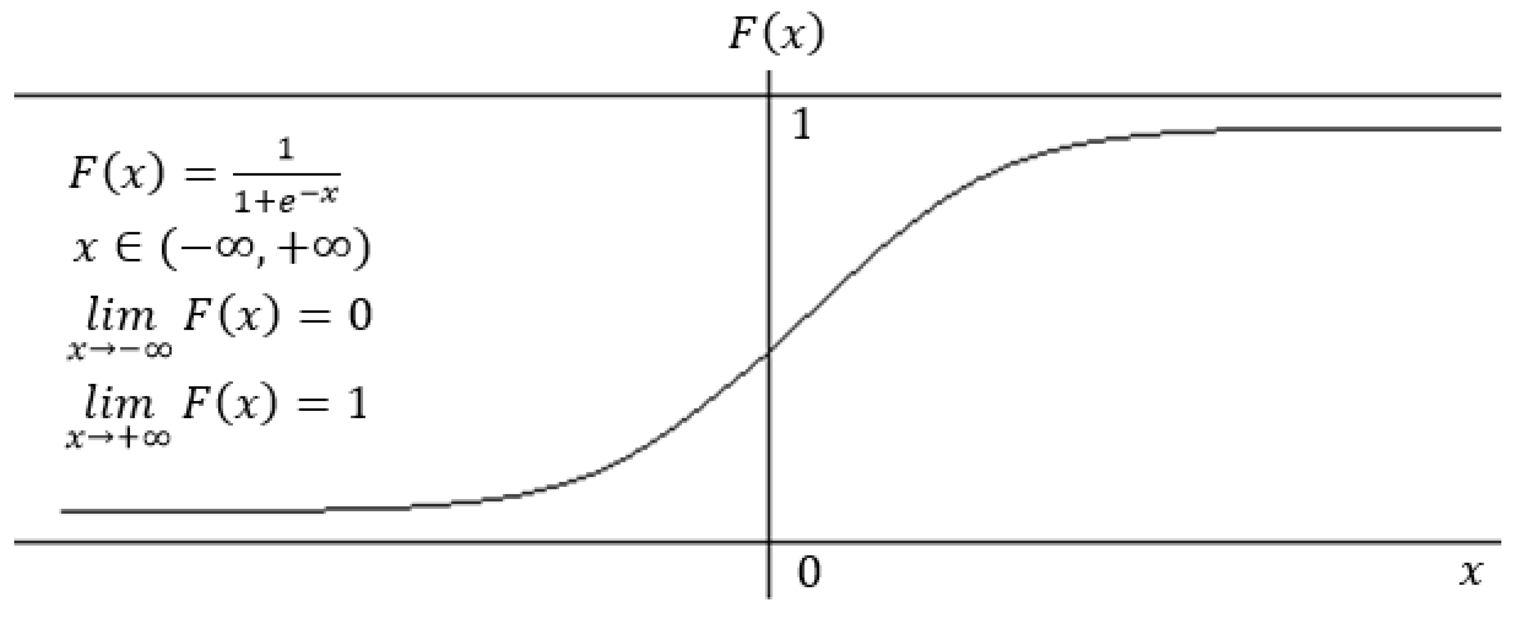
Because the residual item $a_t$ has a strong impact on the prediction value of the return index $r_t$, it is important to predict the trend of the residual item $a_t$. When we define

$$q_t^{(a)}=\frac{1}{1+e^{-a_t}},\mathrm{or}{a}_t=-\ln (\frac{1}{q_t^{(a)}}-1)$$

Then, the variable $q_t^{(a)}$ can be seen as a probability of $a_t$. Assume the first-order difference is $d{q}_t^{(a)}=q_t^{(a)}-q_{t-1}^{(a)}$, the second-order difference is $d^2{q}_t^{(a)}=d{q}_t^{(a)}-d{q}_{t-1}^{(a)}$, the third-order difference is $d^3{q}_t^{(a)}=d^2{q}_t^{(a)}-d^2{q}_{t-1}^{(a)}$, and the $nth-order$ difference is $d^n{q}_t^{(a)}=d^{n-1}{q}_t^{(a)}-d^{n-1}{q}_{t-1}^{(a)}$, and if the level variable $q_t^{(a)}$ is not the autocorrelation time series, the $nth-order$ difference $d^n{q}_t^{(a)}$ may be the autocorrelation time series, then the higher degree $th-order$ difference $d^n{q}_t^{(a)}$ can be expressed by a regression model as $d^n{q}_t^{(a)}=\omega +{\alpha }_0{q}_{t-1}^{(a)}+{\alpha }_{1}d{q}_{t-1}^{(a)}+\cdots +{\alpha }_{n-1}{d}^{n-1}{q}_{t-1}^{(a)}+{\beta }_1{d}^n{q}_{t-1}^{(a)}+\cdots +{\beta }_p{d}^n{q}_{t-p}^{(a)}+c_t$.

The $th$-order difference $d^n{q}_t^{(a)}$ can also be expressed by a regression model as

$$d^n{q}_t^{(a)}=\omega +{\displaystyle \sum }_{i=0}^{n-1}{\alpha }_i{d}^i{q}_{t-1}^{(a)}+{\displaystyle \sum }_{j=1}^p{\beta }_j{d}^n{q}_{t-j}^{(a)}+c_t$$

Here, the variable $c_t$ is the residual item of the regression model. Then, according to the definition of the difference method, the probability $q_t^{(a)}$ can be predicted by

$$q_t^{(a)}=q_{t-1}^{(a)}+d{q}_{t-1}^{(a)}+d^2{q}_{t-1}^{(a)}+\cdots +d^{n-1}{q}_{t-1}^{(a)}+d^n{q}_t^{(a)}$$

It is important to determine a proper order number, which depends on both the degree of autocorrelation and the probability degree of the residual.

Table 3 has listed the autocorrelation (AC) values and Ljung and Box (1978) statistics and probabilities of the time series differences. When the difference orders of the probability time series $q_t^{(a)}$ are increased, the autocorrelation degrees of the related time series will be increased. The autocorrelation of the level time series $q_t^{(a)}$ is $AC(1)=0.001$, which is quite low and the level time series $q_t^{(a)}$ cannot be called an autocorrelation time series. The autocorrelation of the first-order time series $d{q}_t^{(a)}$ is $AC(1)=-0.500$, which is much more than the autocorrelation of the level time series $q_t^{(a)}$. The autocorrelations of the second-order, third-order, and fourth-order difference time series $d^2{q}_t^{(a)}$, $d^3{q}_t^{(a)}$, $d^4{q}_t^{(a)}$ are $AC(1)=-0.667$, $AC(1)=-0.750$, and $AC(1)=-0.800$, respectively. Obviously, the second-order, third-order, and fourth-order difference time series have a higher degree of autocorrelation.

The probability prediction models from the second-order difference are

$$\begin{gathered} d^2{q}_t^{(a)}=0.500528-1.001057q_{t-1}^{(a)}-0.999412d{q}_{t-1}^{(a)} \\ {R}^2=0.8332,S.E.=0.0023,AIC=-9.2381,SIC=-9.2276 \\ {q}_t^{(a)}=q_{t-1}^{(a)}+d{q}_{t-1}^{(a)}+d^2{q}_{t-1}^{(a)} \end{gathered}$$

The probability prediction models from the third-order difference are

$$\begin{gathered} d^3{q}_t^{(a)}=0.502031-1.004064q_{t-1}^{(a)}-0.993302d{q}_{t-1}^{(a)}-1.002993d^2{q}_{t-1}^{(a)} \\ {R}^2=0.9499,S.E.=0.0023,AIC=-9.2362,SIC=-9.2222 \\ {q}_t^{(a)}=q_{t-1}^{(a)}+d{q}_{t-1}^{(a)}+d^2{q}_{t-1}^{(a)}+d^3{q}_{t-1}^{(a)} \end{gathered}$$

The probability prediction models from the fourth-order difference are

$$\begin{gathered} d^4{q}_t^{(a)}=0.502080-1.004163q_{t-1}^{(a)}-0.993244d{q}_{t-1}^{(a)}-1.003043d^2{q}_{t-1}^{(a)}-1.000014d^3{q}_{t-1}^{(a)} \\ {R}^2=0.9857,S.E.=0.0023,AIC=-9.2343,SIC=-9.2168 \\ {q}_t^{(a)}=q_{t-1}^{(a)}+d{q}_{t-1}^{(a)}+d^2{q}_{t-1}^{(a)}+d^3{q}_{t-1}^{(a)}+d^4{q}_{t-1}^{(a)} \end{gathered}$$

After obtaining the prediction value of $q_t^{(a)}$, the prediction value of the return index $r_t$ will be estimated by

$$r_{a,t}={\mu }_{a,t}-\ln (\frac{1}{q_t^{(a)}}-1)$$

By applying the equation, it is easy to obtain the prediction value of the return index $r_t$.

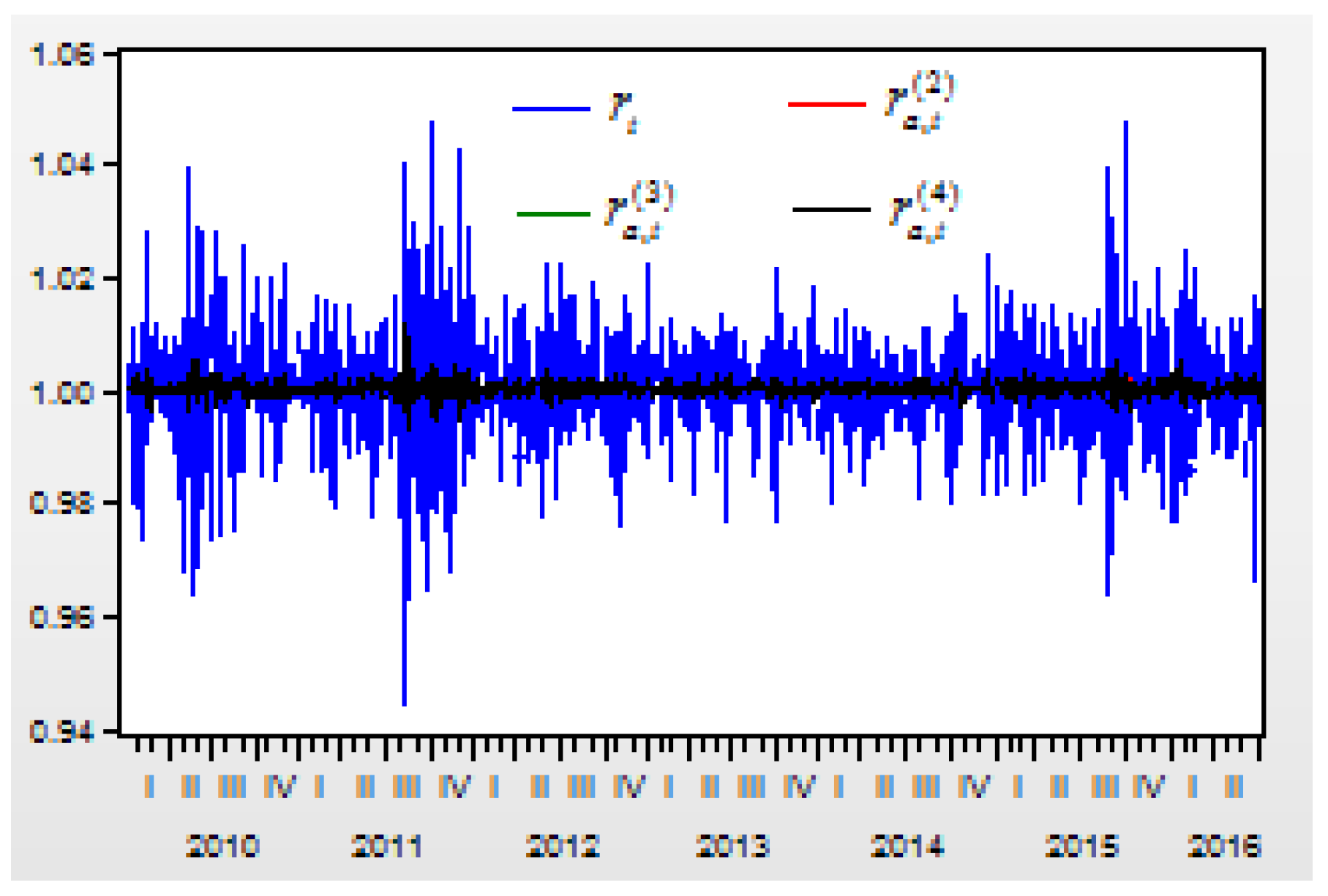
Assume variable ${\mu }_{a,t}$ is the conditional mean from the autoregressive model $r_{a,t}={\mu }_{a,t}+a_t$ when $a_t=0$ or $q_t^{(a)}=0.5$. When $a_t\ne 0$, assume variable $r_{a,t}^{(2)}$ represents the prediction index of the return index $r_t$ from the second-order difference variable $d^2{q}_t^{(a)}$; variable $r_{a,t}^{(3)}$ represents the prediction index of the return index $r_t$ from the third-order difference variable $d^3{q}_t^{(a)}$; and variable $r_{a,t}^{(4)}$ represents the prediction index of the return index $r_t$ from the fourth-order difference variable $d^4{q}_t^{(a)}$.

Figure 4 shows the return index $r_t$ and its prediction values of $r_{a,t}^{(2)}$, $r_{a,t}^{(3)}$, and $r_{a,t}^{(4)}$ from the second-, third-, and fourth-order differences.

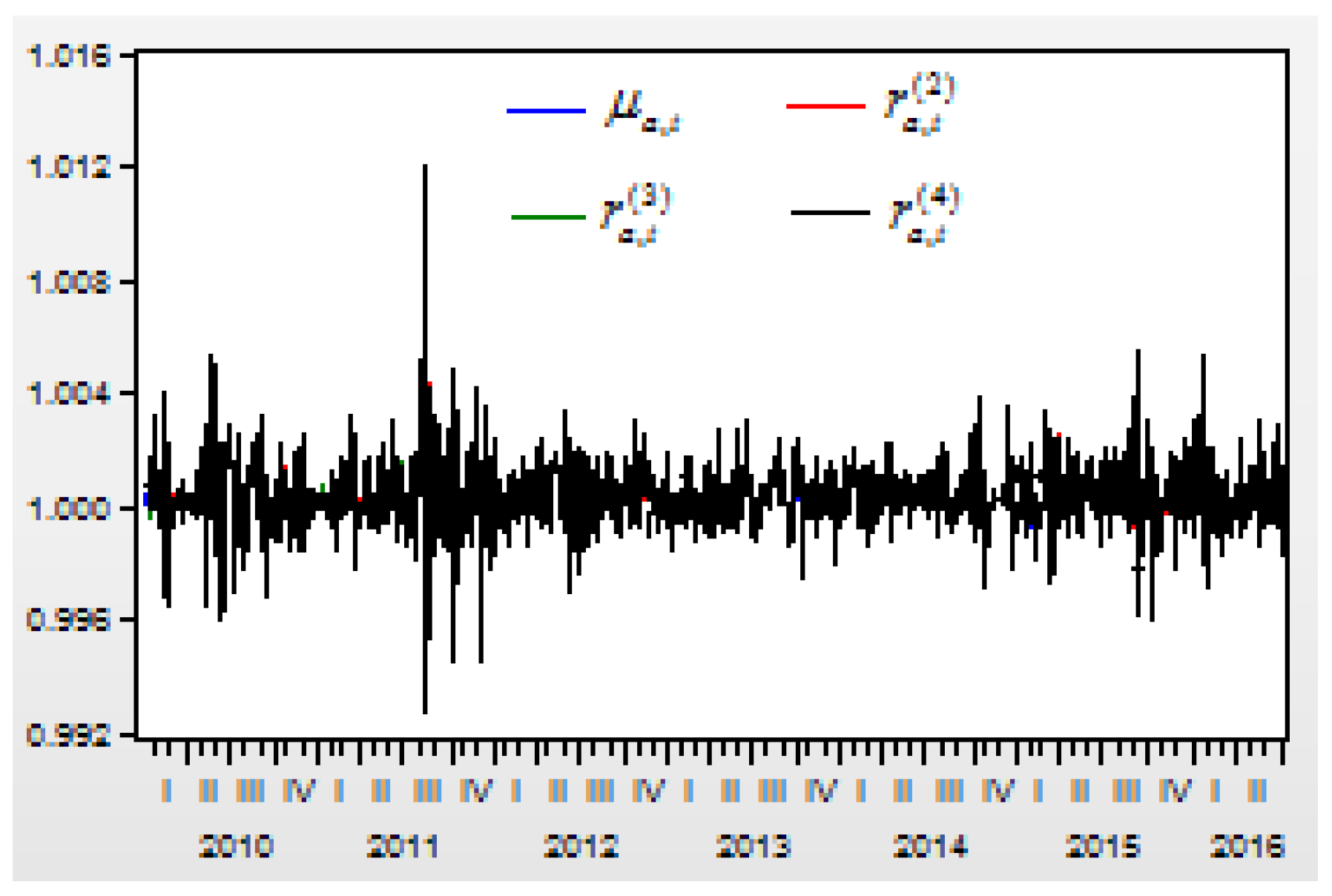
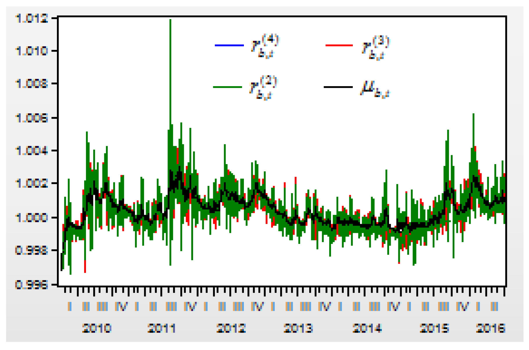
Figure 5 shows the prediction values of $r_{a,t}^{(2)}$, $r_{a,t}^{(3)}$, and $r_{a,t}^{(4)}$ under the second-, third-, and fourth-order differences, and the conditional mean ${\mu }_{a,t}$ of $r_t$.

The correlation between the return index $r_t$ and its conditional mean ${\mu }_{a,t}$, and its prediction values of $r_{a,t}^{(2)}$, $r_{a,t}^{(3)}$, and $r_{a,t}^{(4)}$ are 0.136470, 0.136472, 0.136519, 0.13652, respectively.

For improving the correlations between the return index $r_t$ and its prediction values, we will try to improve the lag order of the finite order differences’ variables.

$$\begin{array}{cc}\hfill d^2{q}_t^{(a)}=& 0.5073-1.0147q_{t-1}^{(a)}-0.9845d{q}_{t-1}^{(a)}-0.0053d^2{q}_{t-1}^{(a)}+0.0023d^2{q}_{t-2}^{(a)}\hfill \\ & +0.0091d^2{q}_{t-3}^{(a)}+0.0147d^2{q}_{t-4}^{(a)}+0.0161d^2{q}_{t-5}^{(a)}+0.0131d^2{q}_{t-6}^{(a)}\hfill \\ & +0.0024d^2{q}_{t-7}^{(a)}+0.0316d^2{q}_{t-8}^{(a)}+0.0664d^2{q}_{t-9}^{(a)}\hfill \\ & +0.0914d^2{q}_{t-10}^{(a)}-0.0720d^2{q}_{t-11}^{(a)}+0.0454d^2{q}_{t-12}^{(a)}\hfill \end{array}$$

$$\begin{array}{cc}\hfill d^3{q}_t^{(a)}=& 0.5184-1.0368q_{t-1}^{(a)}-0.6148d{q}_{t-1}^{(a)}-3.7711d^2{q}_{t-1}^{(a)}+2.4176d^3{q}_{t-1}^{(a)}\hfill \\ & +2.0949d^3{q}_{t-2}^{(a)}+1.8025d^3{q}_{t-3}^{(a)}+1.5403d^3{q}_{t-4}^{(a)}+1.3043d^3{q}_{t-5}^{(a)}\hfill \\ & +1.0923d^3{q}_{t-6}^{(a)}+0.8974d^3{q}_{t-7}^{(a)}+0.6973d^3{q}_{t-8}^{(a)}+0.4900d^3{q}_{t-9}^{(a)}\hfill \\ & +0.2860d^3{q}_{t-10}^{(a)}+0.1297d^3{q}_{t-11}^{(a)}+0.0279d^3{q}_{t-12}^{(a)}\hfill \end{array}$$

$$\begin{array}{cc}\hfill d^4{q}_t^{(a)}=& 0.5376-1.0752q_{t-1}^{(a)}-0.0179d{q}_{t-1}^{(a)}-8.0777d^2{q}_{t-1}^{(a)}+30.61d^3{q}_{t-1}^{(a)}\hfill \\ & +25.44d^4{q}_{t-1}^{(a)}+20.13d^4{q}_{t-2}^{(a)}-15.59d^4{q}_{t-3}^{(a)}-11.77d^4{q}_{t-4}^{(a)}\hfill \\ & -8.60d^4{q}_{t-5}^{(a)}-6.01d^4{q}_{t-6}^{(a)}-3.95d^4{q}_{t-7}^{(a)}-2.38d^4{q}_{t-8}^{(a)}\hfill \\ & -1.27d^4{q}_{t-9}^{(a)}-0.57d^4{q}_{t-10}^{(a)}-0.19d^4{q}_{t-11}^{(a)}-0.04d^4{q}_{t-12}^{(a)}\hfill \end{array}$$

After improving the lag order of the finite order differences’ variables, when $a_t\ne 0$, assume variable $r_{a,t}^{(2^{\prime })}$ represents the prediction index of the return index from $r_t$ the second-order difference variable $d^2{q}_t^{(a)}$; variable $r_{a,t}^{(3^{\prime })}$ represents the prediction index of the return index $r_t$ from the third-order difference variable $d^3{q}_t^{(a)}$; and variable $r_{a,t}^{(4^{\prime })}$ represents the prediction index of the return index $r_t$ from the fourth-order difference variable $d^4{q}_t^{(a)}$. Then, there is a correlation between the return index $r_t$ and its conditional mean ${\mu }_{a,t}$, and its prediction values of $r_{a,t}^{(2^{\prime })}$, $r_{a,t}^{(3^{\prime })}$, $r_{a,t}^{(4^{\prime })}$ are 0.136470, 0.156046, 0.158559, 0.163743, respectively. Obviously, improving the lag order of the finite order differences’ variables can improve the correlations between the return index and its prediction value a lot.

4.5. Return Index Prediction Based on the Second-Order Difference and the AR-FD Model

From the above empirical analysis, we find that if we increasingly improve the order of the finite order differences’ variables, the correlations between the return index and its prediction value cannot increase more and more. We will focus on conducting an analysis on the second-order finite difference regression model and test if higher lags of the probability variable $q_t^{(a)}$ can lead to a higher correlation between the real return index $r_t$ and its prediction value.

The second-order finite difference $d^2{q}_t^{(a)}$ can be expressed as

$$d^2{q}_t^{(a)}=\omega +{\alpha }_0{q}_{t-1}^{(a)}+{\alpha }_{1}d{q}_{t-1}^{(a)}+{\displaystyle \sum }_{j=1}^p{\beta }_j{d}^2{q}_{t-j}^{(a)}+c_t$$

When the lag order of the probability variable $q_t^{(a)}$ is defined as $p=3,50,100,150,200,300,400,500,600,700$, we can obtain ten different prediction models of $d^2{q}_t^{(a)}$. According to the equation of $q_t^{(a)}=q_{t-1}^{(a)}+d{q}_{t-1}^{(a)}+d^2{q}_t^{(a)}$, $r_{a,t}={\mu }_{a,t}-\ln (1/q_t^{(a)}-1)$, we will obtain the return index prediction values of $r_{a,t}{|}_{p=3,50,100,150,200,300,400,500,600,700}$.

Table 4. Results of the second-order finite difference regression models of AR-FD when the lags of the probability are different.

No.	Prediction Model for Second-Order Difference ${\mathit{d}}^2{\mathit{q}}_{\mathit{t}}^{(\mathit{a})}$								${\mathit{r}}_{\mathit{a},\mathit{t}}$	Correlation $\rho ({\mathit{r}}_{\mathit{a},\mathit{t}},{\mathit{r}}_{\mathit{t}})$
	$\mathit{\omega }$	${\mathit{\alpha }}_0$	${\mathit{\alpha }}_1$	$\mathit{p}$	${\mathit{R}}^2$	$\mathit{S}.\mathit{E}.$	$\mathit{A}\mathit{I}\mathit{C}$	$\mathit{S}\mathit{I}\mathit{C}$
1	0.503001	−1.006001	−0.984222	3	0.833302	0.002388	−9.233150	−9.212135	$r_{a,t}{|}_{p=3}$	0.136766
2	0.699362	−1.398724	10.57640	50	0.839955	0.002381	−9.207139	−9.016722	$r_{a,t}{|}_{p=50}$	0.238128
3	0.800919	−1.601812	25.15103	100	0.844830	0.002335	−9.212454	−8.831902	$r_{a,t}{|}_{p=100}$	0.294749
4	0.908183	−1.816307	47.93676	150	0.851597	0.002329	9.181926	−8.600049	$r_{a,t}{|}_{p=150}$	0.341969
5	1.072259	−2.144498	101.5909	200	0.856684	0.002350	−9.128677	−8.333173	$r_{a,t}{|}_{p=200}$	0.389903
6	1.006904	−2.013859	38.47244	300	0.872071	0.002402	−9.014493	−7.749547	$r_{a,t}{|}_{p=300}$	0.486086
7	0.657598	−1.315164	−72.80206	400	0.888580	0.002247	−9.085781	−7.284239	$r_{a,t}{|}_{p=400}$	0.578318
8	1.028349	−2.056674	245.4824	500	0.899775	0.002524	−9.093179	−6.670786	$r_{a,t}{|}_{p=500}$	0.651674
9	1.495949	−2.991754	809.0302	600	0.924362	0.002325	−9.042018	−5.890813	$r_{a,t}{|}_{p=600}$	0.745966
10	1.775340	−3.550546	1191.350	700	0.957954	0.002693	−9.208468	−5.186548	$r_{a,t}{|}_{p=700}$	0.867847

lists the first three parameters of the second-order difference regression models for the residual of the return index prediction model.

When the lag order $p=3$, the regression model of the second-order difference $d^2{q}_t^{(a)}$ includes the intercept $\omega$, and the coefficient ${\alpha }_0$ for item $q_{t-1}^{(a)}$, the coefficient ${\alpha }_1$ for item $d{q}_{t-1}^{(a)}$, and the coefficient ${\beta }_1,{\beta }_2,{\beta }_3$ for item $q_{t-1}^{(a)},q_{t-2}^{(a)},q_{t-3}^{(a)}$.

When the lag order $p=50$, the regression model of the second-order difference $d^2{q}_t^{(a)}$ includes the intercept $\omega$ and the coefficient ${\alpha }_0$ for item $q_{t-1}^{(a)}$, the coefficient ${\alpha }_1$ for item $d{q}_{t-1}^{(a)}$, and the coefficient ${\beta }_1,{\beta }_2,\dots ,{\beta }_{50}$ for item $q_{t-1}^{(a)},q_{t-2}^{(a)},\dots ,q_{t-50}^{(a)}$.

Similarly, when the lag order $p=700$, the regression model of the second-order difference $d^2{q}_t^{(a)}$ includes the intercept $\omega$ and the coefficient ${\alpha }_0$ for item $q_{t-1}^{(a)}$, the coefficient ${\alpha }_1$ for item $d{q}_{t-1}^{(a)}$, and the coefficient ${\beta }_1,{\beta }_2,\dots ,{\beta }_{700}$ for item $q_{t-1}^{(a)},q_{t-2}^{(a)},\dots ,q_{t-700}^{(a)}$.

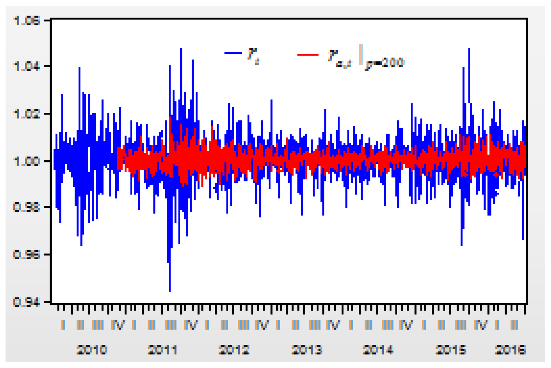
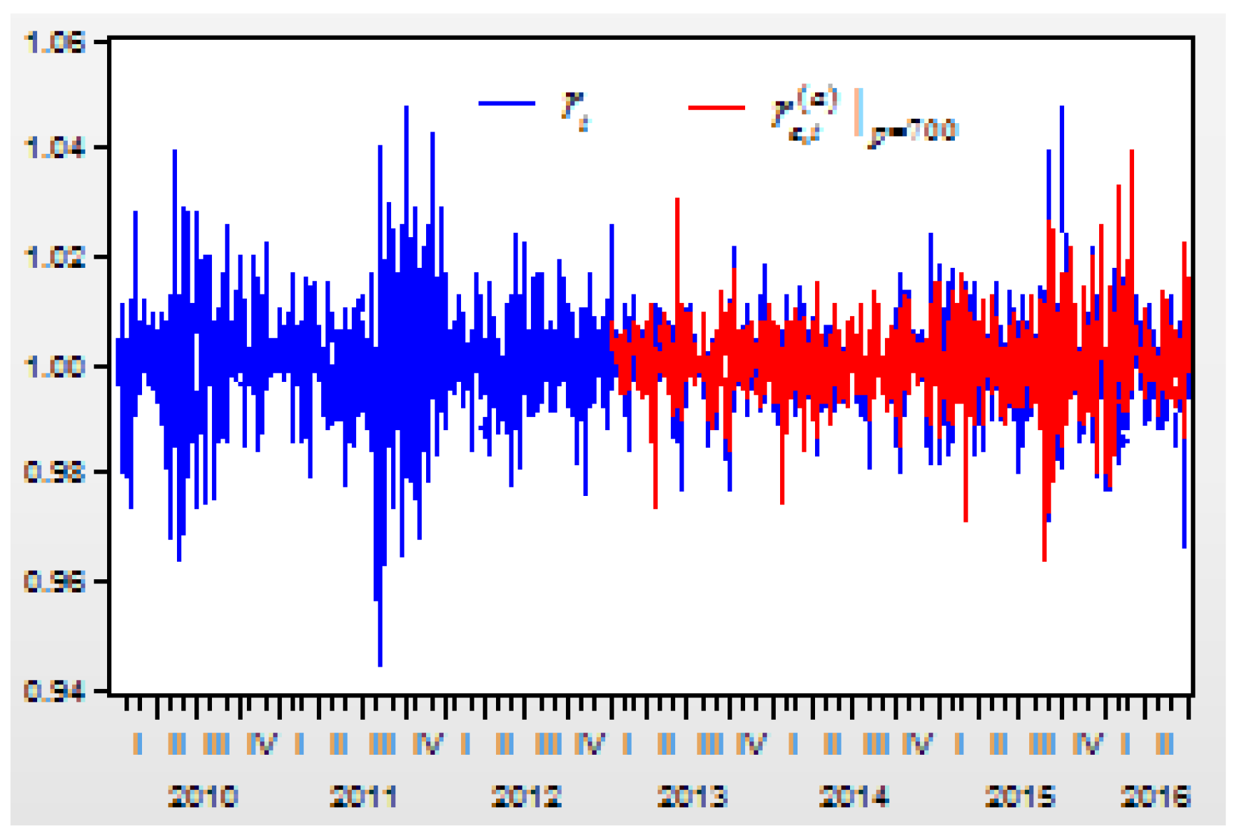
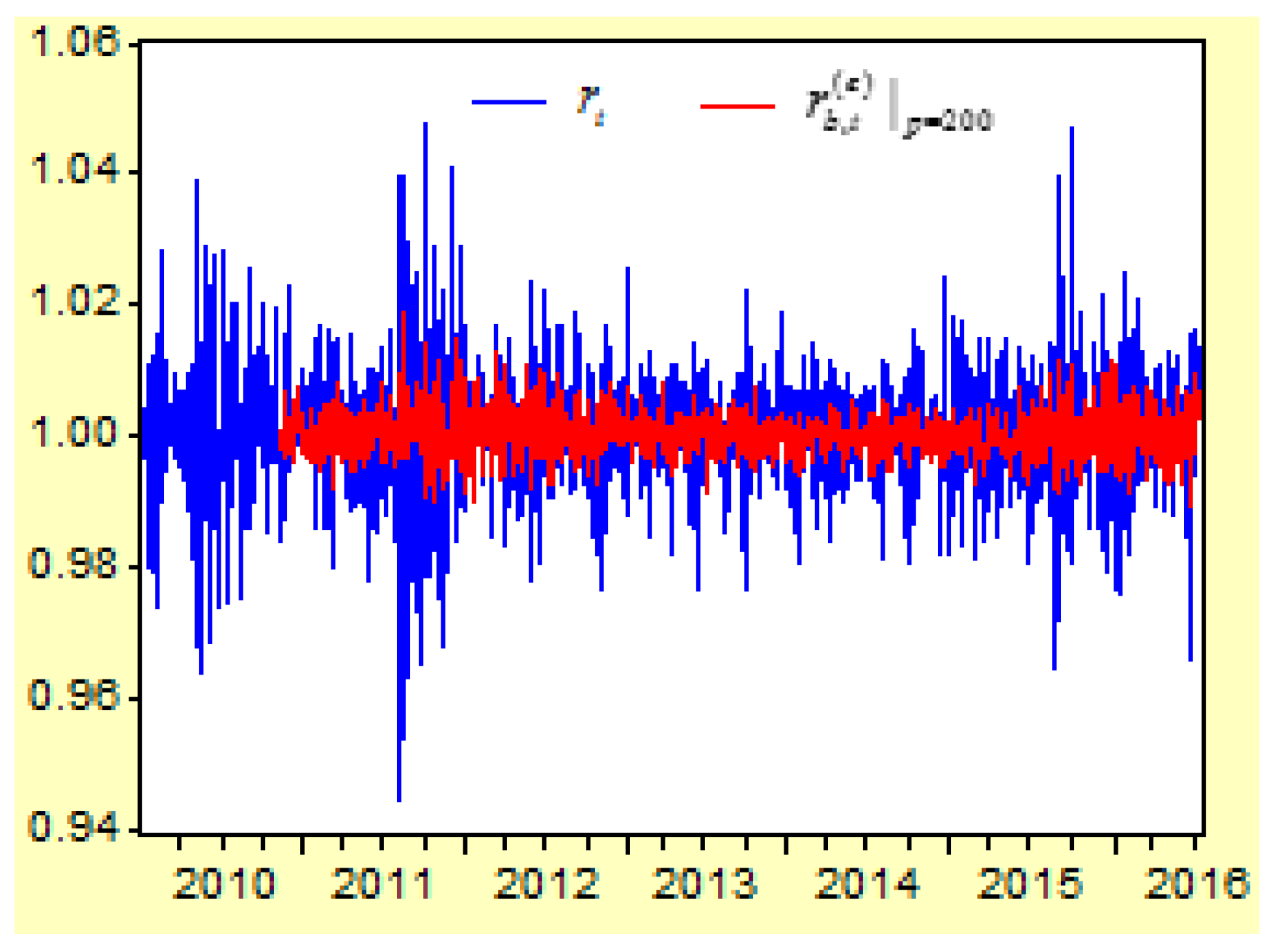
Figure 6 depicts the curves of the return index $r_t$ and its prediction values of $r_{a,t}{|}_{p=200}$ from the second-order difference regression model.

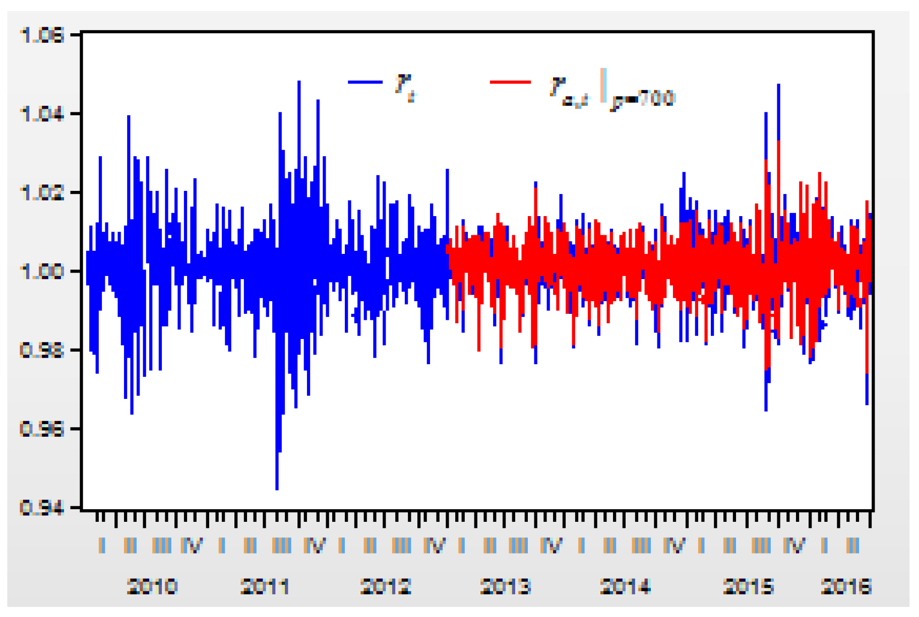
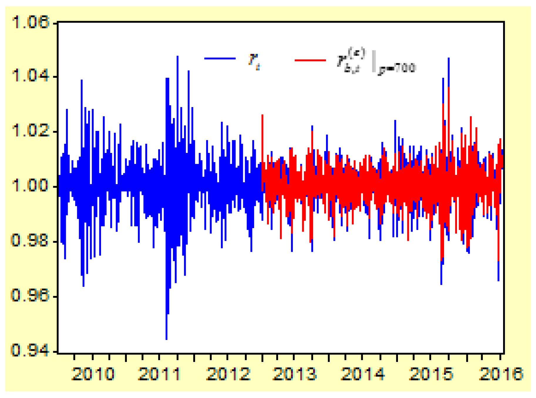
Figure 7 depicts the curves of the return index $r_t$ and its prediction values of $r_{a,t}{|}_{p=700}$ from the second-order difference regression model.

From these regression models for the second-order difference variable $d^2{q}_t^{(a)}$, there are three results:

First, when the lag order of the probability variable $q_t^{(a)}$ increases, the determinate coefficient for the regression model will increase. When the lag order is increased from 3 to 50, 100, 150, 200, 300, 400, 500, 600, and 700, the R-squared value of the regression model is increased from 0.833302 to 0.839955, 0.844830, 0.851597, 0.856684, 0.872071, 0.888580, 0.899775, 0.924362, and 0.957954.

Second, when the lag order increases, the correlations between the real return index $r_t$ and its prediction values will increase. When the lag order is increased from 3 to 50, 100, 150, 200, 300, 400, 500, 600, and 700, the correlation between $r_t$ and its prediction value of $r_{a,t}{|}_{p=3}$, $r_{a,t}{|}_{p=50}$, $r_{a,t}{|}_{p=100}$, $r_{a,t}{|}_{p=150}$, $r_{a,t}{|}_{p=200}$, $r_{a,t}{|}_{p=300}$, $r_{a,t}{|}_{p=400}$, $r_{a,t}{|}_{p=500}$, $r_{a,t}{|}_{p=600}$, $r_{a,t}{|}_{p=700}$ is increased from 0.136766 to 0.238128, 0.294749, 0.341969, 0.389903, 0.486086, 0.578318, 0.651674, 0.745966, and 0. 0.867847, respectively.

Third, when comparing both figures, we can see that the prediction values of $r_{a,t}{|}_{p=700}$ are more approximated to the real return index $r_t$ than the prediction values of $r_{a,t}{|}_{p=200}$. This means that higher lags of the AR-FD prediction model can create a higher approximated result between the real return index $r_t$ and its prediction value.

4.6. GARCH Model

For the residual variable $a_t$, the conditional volatility in the GARCH (1,1) model is regressed as:

$$\begin{gathered} {\sigma }_{a,t}^2=3.65E-06+0.142963a_{t-1}^2+0.819842{\sigma }_{a,t-1}^2 \\ LL=3698.91, AIC=-4.84, SIC=-4.83, HIC=-4.84 \end{gathered}$$

where the static variance is ${\overline{\sigma }}^2=0.009907$, the coefficient of the ARCH item is $\alpha =0.142963>0$, the coefficient of the GARCH item is $\beta =0.819842>0$, the intercept is $\omega =0.00000365>0$, and the three parameters satisfy the relation of $\alpha +\beta =0.962805<1$, $\omega +\alpha +\beta =0.96280865<1$.

The mean and variance of the random variable ${\epsilon }_{a,t}=a_t/{\sigma }_{a,t}$ are −0.008643 and 1.000669, respectively. When the new standardized random variable is defined by $e_{a,t}=({\epsilon }_{a,t}-{\mu }_{a,0})/{\sigma }_{a,0}$, the mean and variance of the random variable $e_{a,t}$ are 3.86E-17 and 1.000328, respectively. Obviously, the random variable $e_{a,t}$ is more approximate to the standardized normal distribution than the random variable ${\epsilon }_{a,t}$.

4.7. Return Index Prediction Based on the Second-Order Finite Difference AR-GARCH-FD Model

When ${\mu }_{a,0}=mean({\epsilon }_{a,t})$, ${\sigma }_{a,0}=\sqrt{\mathrm{Var}({\epsilon }_{a,t})}$, the residual item can be defined as ${\epsilon }_t={\mu }_{0,t}+{\sigma }_{0,t}{e}_{a,t}$, then the autoregressive prediction model of the return index $r_t$ is

$$r_{a,t}={\mu }_{a,t}+{\sigma }_{a,t}({\mu }_{a,0}+{\sigma }_{a,0}{e}_{a,t})$$

Generally, when $\mathrm{Var}({\epsilon }_{a,t})\approx 1$, then ${\sigma }_{a,0}=\sqrt{\mathrm{Var}({\epsilon }_{a,t})}$. For simplicity, we will use $\sqrt{\mathrm{Var}({\epsilon }_{a,t})}$ to replace ${\sigma }_{a,0}$. When the variable $q_{a,t}^{(e)}$ represents the probability of the quantile of $e_{a,t}$, let $q_{a,t}^{(e)}=1/(1+e^{-e_{a,t}})$. Assuming that the probability $q_{a,t}^{(e)}$ is the same as the probability of the random variable, the autoregressive prediction model of the return index $r_t$ can be defined by

$$r_{a,t}^{(e)}={\mu }_{a,t}+{\sigma }_{a,t}\left[{\mu }_{a,0}-{\sigma }_{a,0}(\ln (\frac{1}{q_{a,t}^{(e)}}-1))\right]$$

We will test if a higher lag order of the probability variable $q_{a,t}^{(e)}$ regression model can lead to a higher correlation between the real return index $r_t$ and its prediction value. For this purpose, we will focus on conducting an analysis of the second-order finite difference regression model.

The second-order finite difference $d^2{q}_{a,t}^{(e)}$ can be expressed by a regression model as

$$d^2{q}_{a,t}^{(e)}=\omega +{\alpha }_0{q}_{a,t-1}^{(e)}+{\alpha }_{1}d{q}_{a,t-1}^{(a)}+{{\displaystyle \sum }}_{j=1}^p{\beta }_j{d}^2{q}_{a,t-j}^{(e)}+c_t$$

When the lag order is $p=3,50,100,150,200,300,400,500,600,700$, we can obtain ten different prediction regression models for the second-order finite difference $d^2{q}_{a,t}^{(e)}$.

According to the second-order finite difference equation $q_{a,t}^{(e)}=q_{a,t-1}^{(e)}+d{q}_{a,t-1}^{(e)}+d^2{q}_{a,t}^{(e)}$, the return index prediction regression model $r_{a,t}^{(e)}={\mu }_{a,t}+{\sigma }_{a,t}(mean({\epsilon }_{a,t})+\mathrm{Var}({\epsilon }_{a,t})(-\ln (1/q_{a,t}^{(e)}-1)))$, we will be able to obtain the return index prediction values of $r_{a,t}^{(e)}{|}_{p=3,50,100,150,200,300,400,500,600,700}$.

Table 5. Results of the second-order finite difference regression models of AR-GARCH-FD when the lags of the probability are different.

No.	Prediction Model for Second-Order Difference ${\mathit{d}}^2{\mathit{q}}_{\mathit{a},\mathit{t}}^{(\mathit{e})}$								${\mathit{r}}_{\mathit{a},\mathit{t}}^{(\mathit{e})}$	Correlation $\rho ({\mathit{r}}_{\mathit{a},\mathit{t}}^{(\mathit{e})},{\mathit{r}}_{\mathit{t}})$
	$\mathit{\omega }$	${\mathit{\alpha }}_0$	${\mathit{\alpha }}_1$	$\mathit{p}$	${\mathit{R}}^2$	$\mathit{S}.\mathit{E}.$	$\mathit{A}\mathit{I}\mathit{C}$	$\mathit{S}\mathit{I}\mathit{C}$
1	0.469779	−0.932678	−1.158642	3	0.833870	0.200776	−0.369317	−0.348303	$r_{a,t}^{(e)}{|}_{p=3}$	0.119018
2	0.589021	−1.170411	4.081024	50	0.837518	0.202060	−0.325208	−0.134791	$r_{a,t}^{(e)}{|}_{p=50}$	0.209055
3	0.628908	−1.248931	11.11614	100	0.843600	0.200978	−0.301658	0.078894	$r_{a,t}^{(e)}{|}_{p=100}$	0.268237
4	0.581813	−1.153323	3.988102	150	0.849075	0.202184	−0.254624	0.327253	$r_{a,t}^{(e)}{|}_{p=150}$	0.315291
5	0.731301	−1.453786	52.43478	200	0.853597	0.203925	−0.201919	0.593585	$r_{a,t}^{(e)}{|}_{p=200}$	0.367438
6	0.760529	−1.516576	54.26585	300	0.869262	0.206495	−0.106405	1.158541	$r_{a,t}^{(e)}{|}_{p=300}$	0.472224
7	0.821250	−1.628421	172.4720	400	0.887668	0.206334	−0.045567	1.755975	$r_{a,t}^{(e)}{|}_{p=400}$	0.552860
8	0.999699	−1.986074	296.8563	500	0.905421	0.210893	0.031770	2.454163	$r_{a,t}^{(e)}{|}_{p=500}$	0.640771
9	1.493677	−2.955449	783.0487	600	0.930127	0.220599	0.062982	3.214187	$r_{a,t}^{(e)}{|}_{p=600}$	0.701112
10	1.459492	−2.890825	827.5364	700	0.962585	0.248488	−0.158915	3.863005	$r_{a,t}^{(e)}{|}_{p=700}$	0.847974

lists the first three parameters of the second-order finite difference regression models for different lags of the probability from the residual of the return index prediction model.

When the lag order $p=3$, the regression model of the second-order difference $d^2{q}_{a,t}^{(e)}$ includes the intercept $\omega$ and the coefficient ${\alpha }_0$ for item $q_{a,t-1}^{(e)}$, the coefficient ${\alpha }_1$ for item $d{q}_{a,t}^{(e)}$, and the coefficient ${\beta }_1, {\beta }_2,{\beta }_3$ for item $q_{a,t-1}^{(e)}, q_{a,t-2}^{(e)},q_{a,t-3}^{(e)}$.

When the lag order $p=50$, the regression model of the second-order difference $d^2{q}_{a,t}^{(e)}$ includes the intercept $\omega$ and the coefficient ${\alpha }_0$ for item $q_{a,t-1}^{(e)}$, the coefficient ${\alpha }_1$ for item $d{q}_{a,t}^{(e)}$, and the coefficient ${\beta }_1, {\beta }_2,\dots ,{\beta }_{50}$ for item $q_{a,t-1}^{(e)}, q_{a,t-2}^{(e)},q_{a,t-50}^{(e)}$.

Similarly, When the lag order $p=700$, the regression model of the second-order difference $d^2{q}_{a,t}^{(e)}$ includes the intercept $\omega$ and the coefficient ${\alpha }_0$ for item $q_{a,t-1}^{(e)}$, the coefficient ${\alpha }_1$ for item $d{q}_{a,t}^{(e)}$, and the coefficient ${\beta }_1, {\beta }_2,\dots ,{\beta }_{700}$ for item $q_{a,t-1}^{(e)}, q_{a,t-2}^{(e)},q_{a,t-700}^{(e)}$.

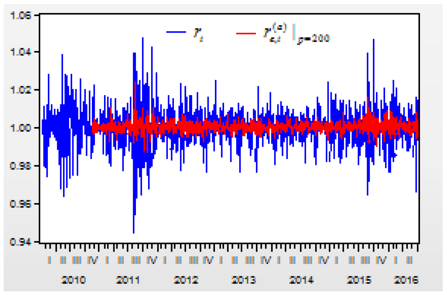
Figure 8 depicts the curves of the return index $r_t$ and its prediction values of $r_{a,t}^{(e)}{|}_{p=200}$ from the second-order difference regression model.

Figure 9 depicts the curves of the return index $r_t$ and its prediction values of $r_{a,t}^{(e)}{|}_{p=700}$ from the second-order difference regression model.

From these regression models for the second-order difference variable $d^2{q}_t^{(e)}$, there are three results:

First, when the lag order increases, the determinate coefficient for the regression model will increase. When the lag order is increased from 3 to 50, 100, 150, 200, 300, 400, 500, 600, and 700, the R-squared value of the regression model is increased from 0.833870 to 0.837518, 0.843600, 0.849075, 0.853597, 0.869262, 0.887668, 0.905421, 0.930127, and 0.962585.

Secondly, when the lag order increases, the correlations between the real return index $r_t$ and its prediction values will increase. When the lag order is increased from 3 to 50, 100, 150, 200, 300, 400, 500, 600, and 700, the correlation between $r_t$ and its prediction values of $r_{a,t}^{(e)}{|}_{p=3}$, $r_{a,t}^{(e)}{|}_{p=50}$, $r_{a,t}^{(e)}{|}_{p=100}$, $r_{a,t}^{(e)}{|}_{p=150}$, $r_{a,t}^{(e)}{|}_{p=200}$, $r_{a,t}^{(e)}{|}_{p=300}$, $r_{a,t}^{(e)}{|}_{p=400}$, $r_{a,t}^{(e)}{|}_{p=500}$, $r_{a,t}^{(e)}{|}_{p=600}$, $r_{a,t}^{(e)}{|}_{p=700}$ increases from 0.119018 to 0.209055, 0.268237, 0.315291, 0.367438, 0.472224, 0.552860, 0.640771, 0.701112, and 0.847974, respectively.

Thirdly, when comparing both figures, we can see that the prediction values of $r_{a,t}^{(e)}{|}_{p=700}$ are more approximated to the real return index $r_t$ than the prediction values of $r_{a,t}^{(e)}{|}_{p=200}$. This means that higher lags of the AR-GARCH-FD prediction model can create a higher approximated result between the real return index $r_t$ and its prediction value.

5. Empirical Analysis Based on the Cumulative Return Index

5.1. The Cumulative Return Index

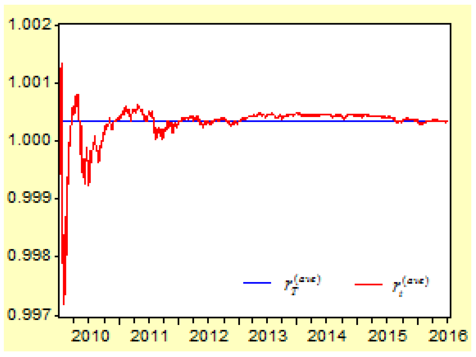
Figure 10 shows the moving curves of the average compound return index $r_t^{(ave)}$ between the time period $t\in \left[0,t\right]$ and the average compound return index $r_T^{(ave)}$ when $t=T$ between 4 January 2010 and 8 July 2016.

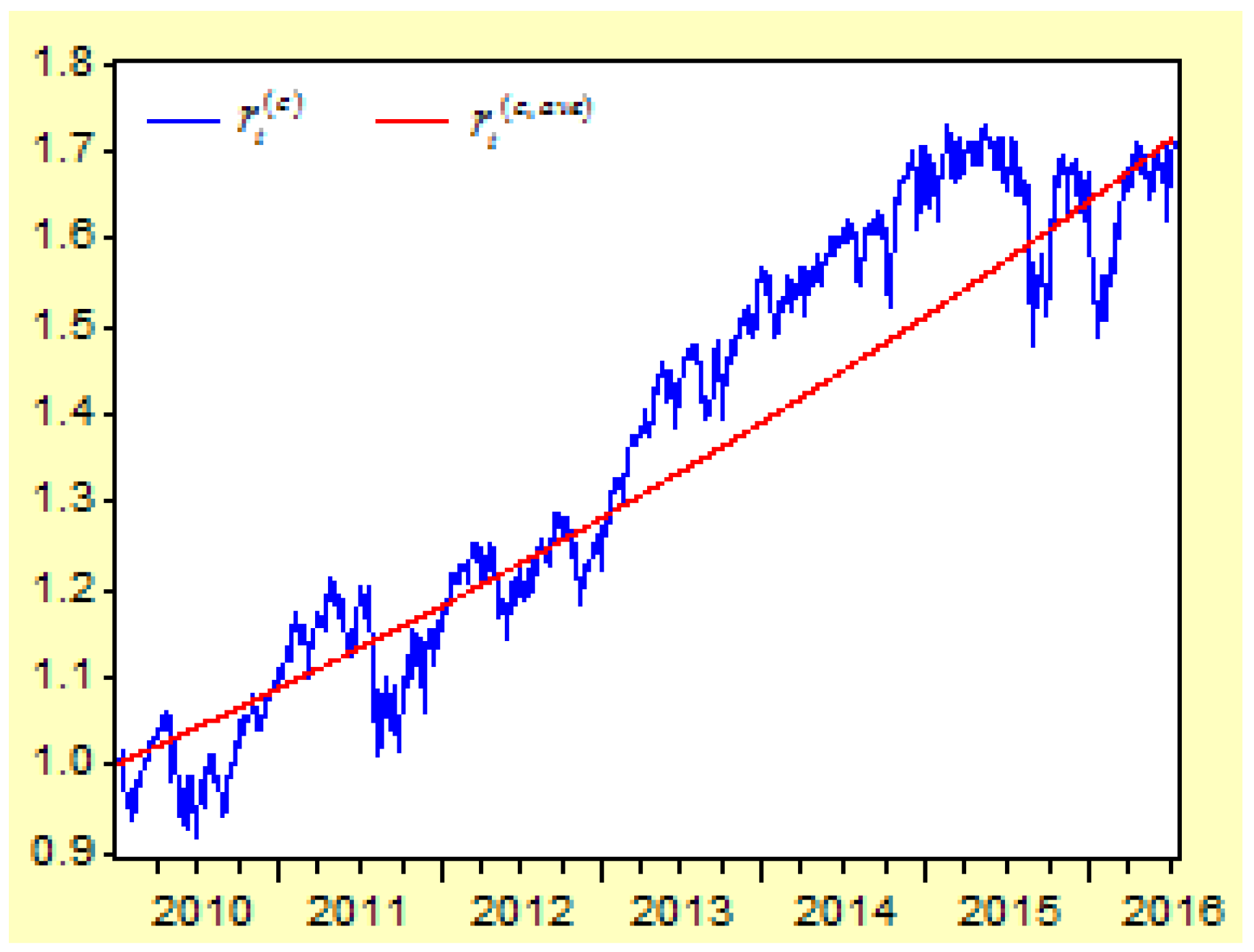
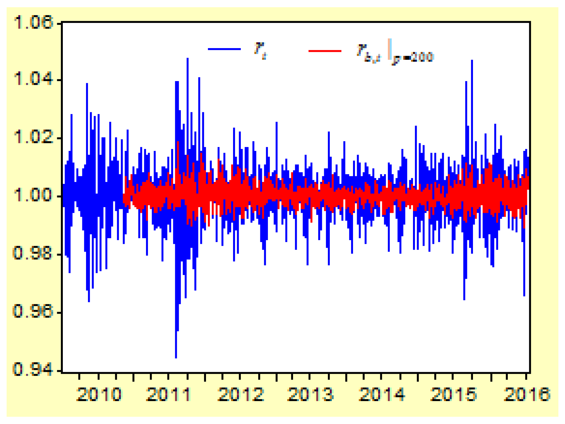
Figure 11 shows the cumulative return index $r_t^{(c)}$ and the cumulative average compound return index $r_t^{(c,ave)}$ between 4 January 2010 and 8 July 2016.

According to statistics, the average arithmetic return index $\overline{r}=1.000398$, and the average compound return index $r_T^{(ave)}={(r_T^{(c)})}^{1/T}=1.000352$. The average arithmetic return index is not equal to the average compound return index. The average compound return index reveals the characteristics of the risk assets’ return indices.

It is clear that the cumulative return index $r_t^{(c)}$ represents the long-term moving trend of the return index $r_t$, and the cumulative average compound return index $r_t^{(c,ave)}$ represents the long-term moving trend of the average compound return index $r_T^{(ave)}$.

When comparing the trends between the short-term return index $r_t$ and the long-term cumulative return index $r_t^{(c)}$, it is obvious that the long-term cumulative return index has a clearer moving trend than the short-term return index. For this reason, we will focus on conducting an analysis of the long-term cumulative return index.

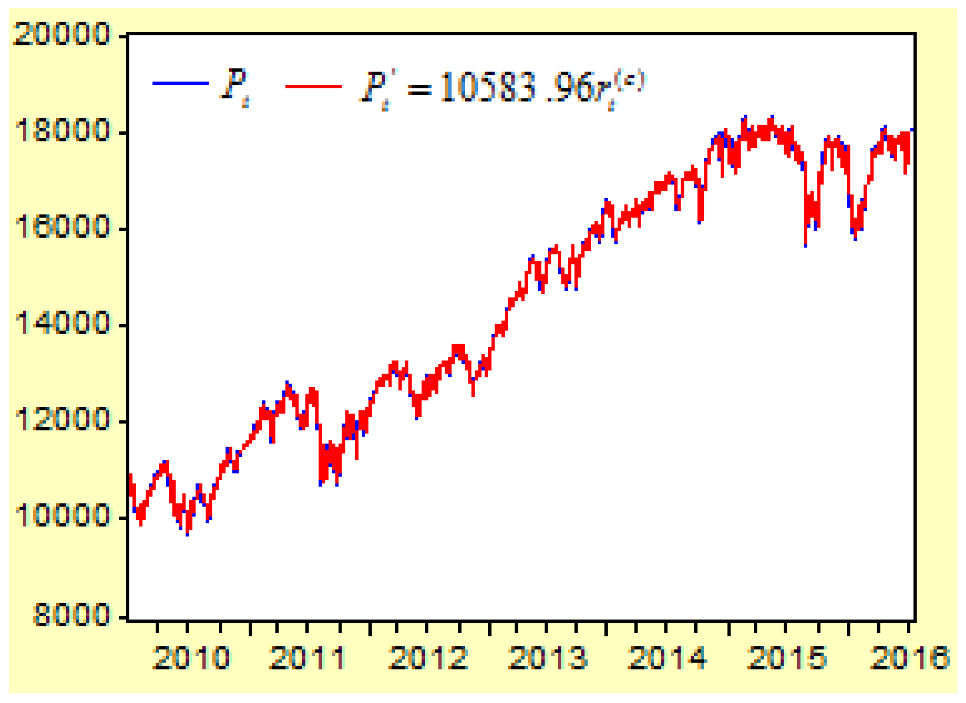
If we have already learned the prediction value of the cumulative return index $r_t^{(c)}$, we will obtain the prediction value of the stock price $P_t^{\prime }=P_0{r}_t^{(c)}$. Because the stock price on the first day (4 January 2010) is $P_0=P_1=10583.96$, if we can predict the value of the cumulative return index $r_t^{(c)}$, the prediction value of the price at any time $t\in \left[1,t\right]$ will be $P_t^{\prime }=P_0{r}_t^{(c)}=10583.96r_t^{(c)}$.

Figure 12 has listed the stock price $P_t$ and its prediction value from the formula $P_t^{\prime }=10583.96r_t^{(c)}$. Because the cumulative return index $r_t^{(c)}$ is from the real value of the return index $r_t$, the curves of both $P_t$ and $P_t^{\prime }=10583.96r_t^{(c)}$ are almost the same.

It is clear from comparing the curves of the cumulative return index $r_t^{(c)}$ and the real return index $r_t$ that the forecasting procedure of the cumulative return index $r_t^{(c)}$ may be much easier than the forecasting procedure of the real return index $r_t$.

5.2. The Cumulative Return Gap Index

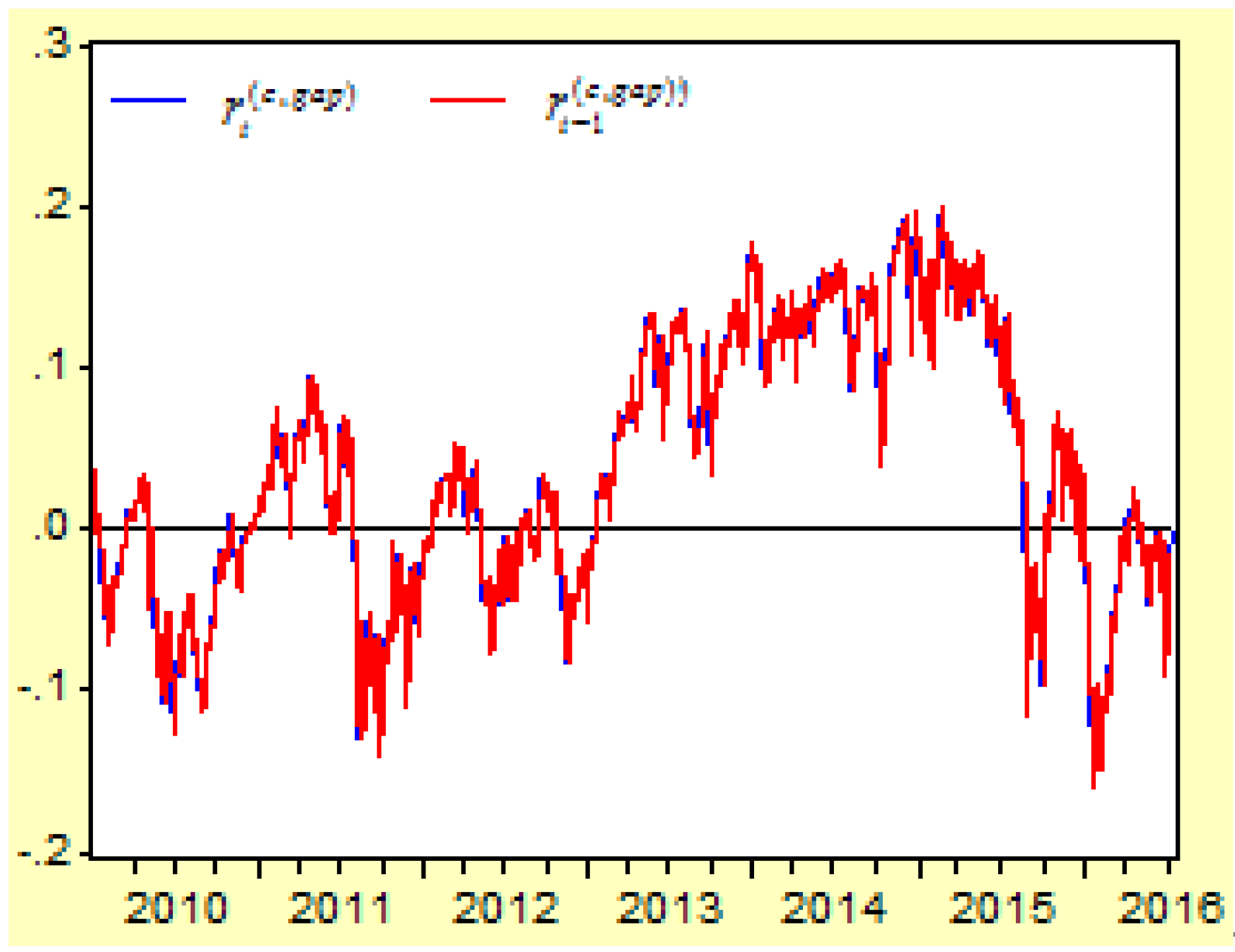
Figure 13 shows the moving curves of the cumulative return gap (CRG) index $r_t^{(c,gap)}$ and its lag 1 item $r_{t-1}^{(c,gap)}$ between 4 January 2010 and 8 July 2016.

The cumulative return gap index $r_t^{(c,gap)}$ represents a long-term cumulative excess return, which has an average arithmetic mean of 0.0375. We can see that it is difficult to differentiate both curves of $r_t^{(c,gap)}$ and its lag 1 item $r_{t-1}^{(c,gap)}$; this is because the time series of the cumulative return gap index $r_t^{(c,gap)}$ has a very high autocorrelation.

The cumulative return gap ($r_t^{(c,gap)}=r_t^{(c)}-r_T^{(c)}$) reveals a cumulative risk premium during the time period of $t\in (0,t)$. When the general risk premium ($r_t^{(gap)}=r_t-r_f$) reveals a difference between the return of a risk asset and the return of a risk-free asset, the cumulative return gap reveals the difference between the cumulative compound return and the cumulative average compound return of a risk asset.

Table 6. Autocorrelation (AC) values and probabilities of Ljung and Box (1978) statistics for the cumulative return gap index.

Variable	AC(1)	P(1)	AC(5)	P(5)	AC(10)	P(10)	AC(15)	P(15)	AC(20)	P(20)	AC(25)	P(25)
$r_t^{(c,gap)}$	0.988	0.000	0.942	0.000	0.897	0.000	0.850	0.000	0.808	0.000	0.769	0.000

lists the autocorrelations and the probabilities of Ljung and Box (1978) statistics for the time series variable $r_t^{(c,gap)}$. The autocorrelation between both time series $r_t^{(c,gap)}$ and $r_{t-1}^{(c,gap)}$ is 0.988, which is much higher than the value of the autocorrelation of −0.052 between the time series $r_t$ and $r_{t-1}$.

Because the correlation between the cumulative return gap index and its lag 1 item is as high as 0.988, or ${\rho }_1=\mathrm{Corr}(r_t^{(c,gap)},r_{t-1}^{(c,gap)})=0.988$, the term of $r_{t-1}^{(c,gap)}$ can be applied into the prediction model to replace the value of $r_t^{(c,gap)}$. We have already learned that the cumulative return index $r_t^{(c)}$ can be depicted as $r_t^{(c)}=r_t^{(c,ave)}+r_t^{(c,gap)}$; if $r_t^{(c,gap)}\approx r_{t-1}^{(c,gap)}$, then $r_t^{(c)}=r_t^{(c,ave)}+r_{t-1}^{(c,gap)}$. For this reason, the expression of $r_t^{(c)}$ will include these two items of $r_t^{(c,ave)}$ and $r_{t-1}^{(c,gap)}$.

5.3. ARDL-CRG Prediction Model for the Cumulative Return Index

According to the definition, the cumulative return index $r_t^{(c)}$ is related to four components: the cumulative average compound return index $r_t^{(c,ave)}$, the time function $f(t)$, the cumulative return gap index $r_{t-1}^{(c,gap)}$, and the residual variable $b_t$. Because the cumulative return gap item $r_{t-1}^{(c,gap)}$ is introduced to the ARDL model, the new model can be called the ARDL-CRG model with the following equation

$$\begin{gathered} r_{b,t}^{(c)}={\mu }_{b,t}^{(c)}+b_t \\ {\mu }_{b,t}^{(c)}=-0.002475+0.998355r_t^{(c,ave)}+0.985347r_{t-1}^{(c,gap)}+0.000818\ln t \\ {R}^2=0.997444, S.E.=0.012508, AIC=-5.922330 \end{gathered}$$

The ARDL-CRG model shows that the dependent variable $r_t^{(c)}$ can be represented by the independent variable $r_t^{(c,ave)}$, $r_{t-1}^{(c,gap)}$, and $\ln t$ very well. The determined coefficient is as high as $R^2=0.997444$.

The coefficient of $r_t^{(c,ave)}$ is 0.998355. The coefficient of $r_{t-1}^{(c,gap)}$ is 0.985347. Both of the coefficients are very close to one. Because the coefficient of $\ln t$ is 0.000818, this means that the long-term trend of the stock market increases when the time variable is moving forward.

When the residual value of $b_t$ is ignored, it is easy to obtain the predicted value ${\mu }_{b,t}^{(c)}$ from this ARDL-CRG model. From the ARDL_CRM model, we can predict the return index by following the equations

$$r_{b,t}={\mu }_{b,t}+b_t^{\prime },\mathrm{where}{\mu }_{b,t}=\frac{{\mu }_{b,t}^{(c)}}{r_{t-1}^{(c)}},b_t^{\prime }=\frac{b_t}{r_{t-1}^{(c)}}$$

Figure 14 shows the return index $r_t$ and its prediction value of ${\mu }_{b,t}$. The prediction value of ${\mu }_{b,t}$ is the conditional mean of $r_t$, which is similar to the equation of $r_{b,t}={\mu }_{b,t}$ when $b_t^{\prime }=0$. The correlation between $r_t$ and ${\mu }_{b,t}$ is 0.0984. Although the correlation is low, it is good for representing the relationship between the return index $r_t$ and the conditional mean ${\mu }_{b,t}$.

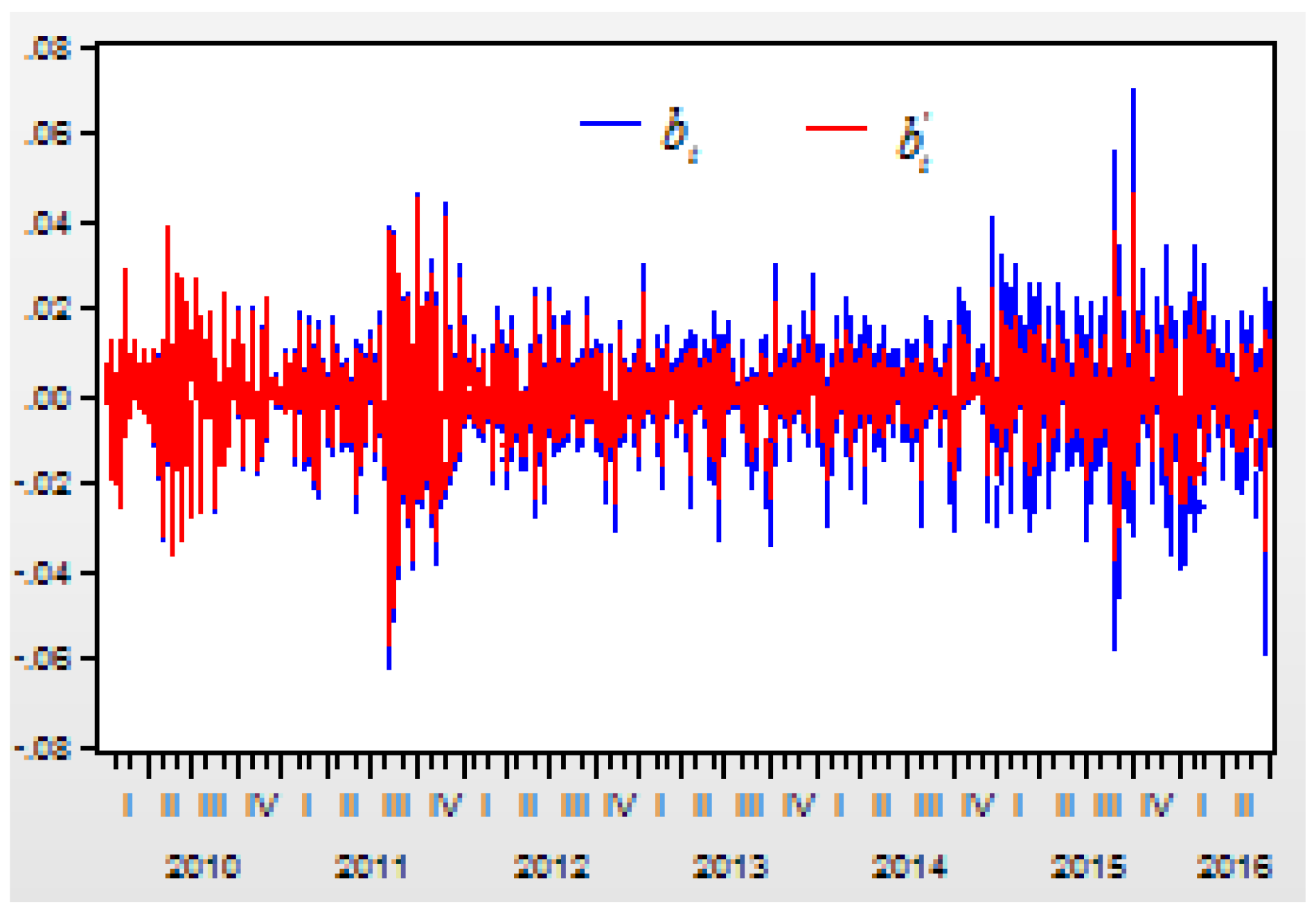
Figure 15 shows the residual $b_t$ from the prediction model of $r_{b,t}^{(c)}={\mu }_{b,t}^{(c)}+b_t$ and the residual $b_t^{\prime }$ from the prediction model of $r_{b,t}={\mu }_{b,t}+b_t^{\prime }$. The correlation between $b_t$ and $b_t^{\prime }$ is 0.9803. The correlation is quite high. It means that the prediction model of the cumulative return index is consistent with the prediction model of the real return index, although the most historic information is included in the residual items.

5.4. Indirect Prediction of the Return Index Based on the Finite Difference Method ARDL-CRG-FD Model

When the finite difference method is introduced into the ARDL-CRG model, the model will become the ARDL-CRG-FD model.

Because the residual item $b_t$ has a strong impact on the prediction value of the cumulative return index $r_t^{(c)}$, it is important to predict the trend of the residual item $b_t$. When defining

$$q_t^{(b)}=\frac{1}{1+e^{-b_t}},\mathrm{or}{b}_t=-\ln (\frac{1}{q_t^{(b)}}-1)$$

then the variable $q_t^{(b)}$ can be seen as a probability of $b_t$. If we assume the first-order difference is $d{q}_t^{(b)}=q_t^{(b)}-q_{t-1}^{(b)}$, the second-order difference is $d^2{q}_t^{(b)}=d{q}_t^{(b)}-d{q}_{t-1}^{(b)}$, the third-order difference is $d^3{q}_t^{(b)}=d^2{q}_t^{(b)}-d^2{q}_{t-1}^{(b)}$, and the $nth-order$ difference is $d^n{q}_t^{(b)}=d^{n-1}{q}_t^{(b)}-d^{n-1}{q}_{t-1}^{(b)}$. If the level variable $q_t^{(b)}$ is not the autocorrelation time series, the $nth-order$ difference $d^n{q}_t^{(b)}$ may be the autocorrelation time series. If the $nth-order$ difference $d^n{q}_t^{(b)}$ can be expressed as

$$d^n{q}_t^{(b)}=\omega +{\alpha }_0{q}_{t-1}^{(b)}+{\alpha }_{1}d{q}_{t-1}^{(b)}+\cdots +{\alpha }_{n-1}{d}^{n-1}{q}_{t-1}^{(b)}+{\beta }_1{d}^n{q}_{t-1}^{(b)}+\cdots +{\beta }_p{d}^n{q}_{t-p}^{(b)}+c_t$$

the $nth$-order difference $d^n{q}_t^{(b)}$ can also be expressed as

$$d^n{q}_t^{(b)}=\omega +{\displaystyle \sum }_{i=0}^{n-1}{\alpha }_i{d}^i{q}_{t-1}^{(b)}+{\displaystyle \sum }_{j=1}^p{\beta }_j{d}^n{q}_{t-j}^{(b)}+c_t$$

Then, according to the definition of the difference method, the probability $q_t^{(b)}$ can be predicted by

$$q_t^{(b)}=q_{t-1}^{(b)}+d{q}_{t-1}^{(b)}+d^2{q}_{t-1}^{(b)}+\cdots +d^{n-1}{q}_{t-1}^{(b)}+d^n{q}_t^{(b)}$$

The variable $c_t$ is the residual item of the regression model. It is important to determine a proper order number; for example, we will consider the first-, second- and fourth-order differences. For simplicity, we will not consider the residual $c_t$ again and assume $c_t=0$.

After obtaining the prediction value of the probability $q_t^{(b)}$, it is easy to obtain the prediction value of the cumulative return index $r_t^{(c)}$ by

$$r_{b,t}^{(c)}={\mu }_{b,t}^{(c)}-\ln (\frac{1}{q_t^{(b)}}-1)$$

By applying the equation of $r_{b,t}=r_{b,t}^{(c)}/r_{t-1}^{(c)}$, it is easy to obtain the prediction value of the return index $r_t$.

The probability prediction models from the second-order difference are

$$\begin{gathered} d^2{q}_t^{(b)}=0.563364-1.126737q_{t-1}^{(b)}-0.675543d{q}_{t-1}^{(b)}-0.225449d^2{q}_{t-1}^{(b)}-0.103285d^2{q}_{t-2}^{(b)}-0.051688d^2{q}_{t-3}^{(b)} \\ {R}^2=0.8426, S.E.=0.0031, AIC=-8.6992, SIC=8.6782 \\ {q}_t^{(b)}=q_{t-1}^{(b)}+d{q}_{t-1}^{(b)}+d^2{q}_t^{(b)} \end{gathered}$$

The probability prediction models from the third-order difference are

$$\begin{gathered} d^3{q}_t^{(b)}=0.563364-1.126737q_{t-1}^{(b)}-0.675543d{q}_{t-1}^{(b)}-1.380421d^2{q}_{t-1}^{(b)}+0.154973d^3{q}_{t-1}^{(b)}+0.051688d^3{q}_{t-2}^{(b)} \\ {R}^2=0.9536, S.E.=0.0031, AIC=-8.6992, SIC=-8.6782 \\ {q}_t^{(b)}=q_{t-1}^{(b)}+d{q}_{t-1}^{(b)}+d^2{q}_{t-1}^{(b)}+d^3{q}_t^{(b)} \end{gathered}$$

The probability prediction models from the fourth-order difference are

$$\begin{gathered} d^4{q}_t^{(b)}=0.563364-1.126737q_{t-1}^{(b)}-0.675543d{q}_{t-1}^{(b)}-1.380421d^2{q}_{t-1}^{(b)}-0.793340d^3{q}_{t-1}^{(b)}-0.051688d^4{q}_{t-1}^{(b)} \\ {R}^2=0.9869, S.E.=0.0031, AIC=-8.6992, SIC=-8.6782 \\ {q}_t^{(b)}=q_{t-1}^{(b)}+d{q}_{t-1}^{(b)}+d^2{q}_{t-1}^{(b)}+d^3{q}_{t-1}^{(b)}+d^4{q}_t^{(b)} \end{gathered}$$

Assume variable $r_{b,t}^{(2)}$ represents the prediction value of the return index $r_t$ from the second-order difference probability prediction value of $q_t^{(b)}$; variable $r_{b,t}^{(3)}$ represents the prediction value of the return index $r_t$ from the third-order difference probability prediction value of $q_t^{(b)}$; and variable $r_{b,t}^{(4)}$ represents the prediction value of the return index $r_t$ from the fourth-order difference probability prediction value of $q_t^{(b)}$.

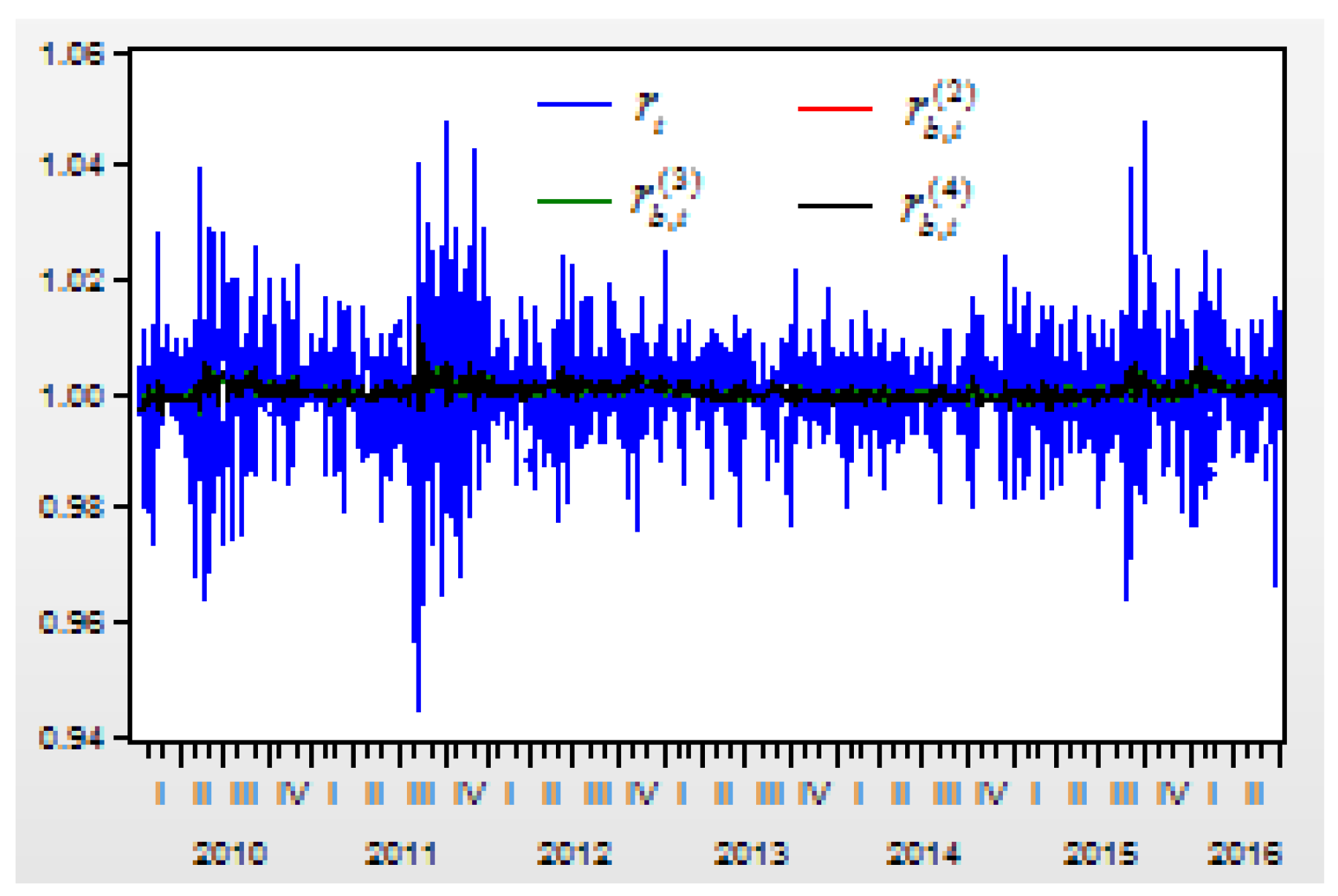
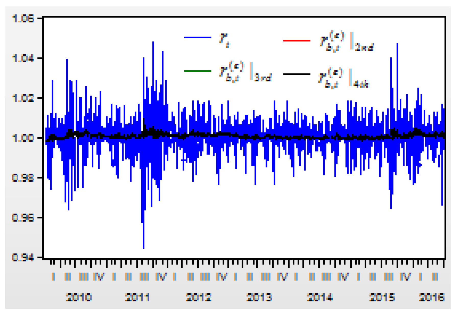
Figure 16 shows the curves of the return index $r_t$ and its prediction values of $r_{b,t}^{(2)}$, $r_{b,t}^{(3)}$, and $r_{b,t}^{(4)}$ from the second, third and fourth difference probability prediction values during 2010–2016.

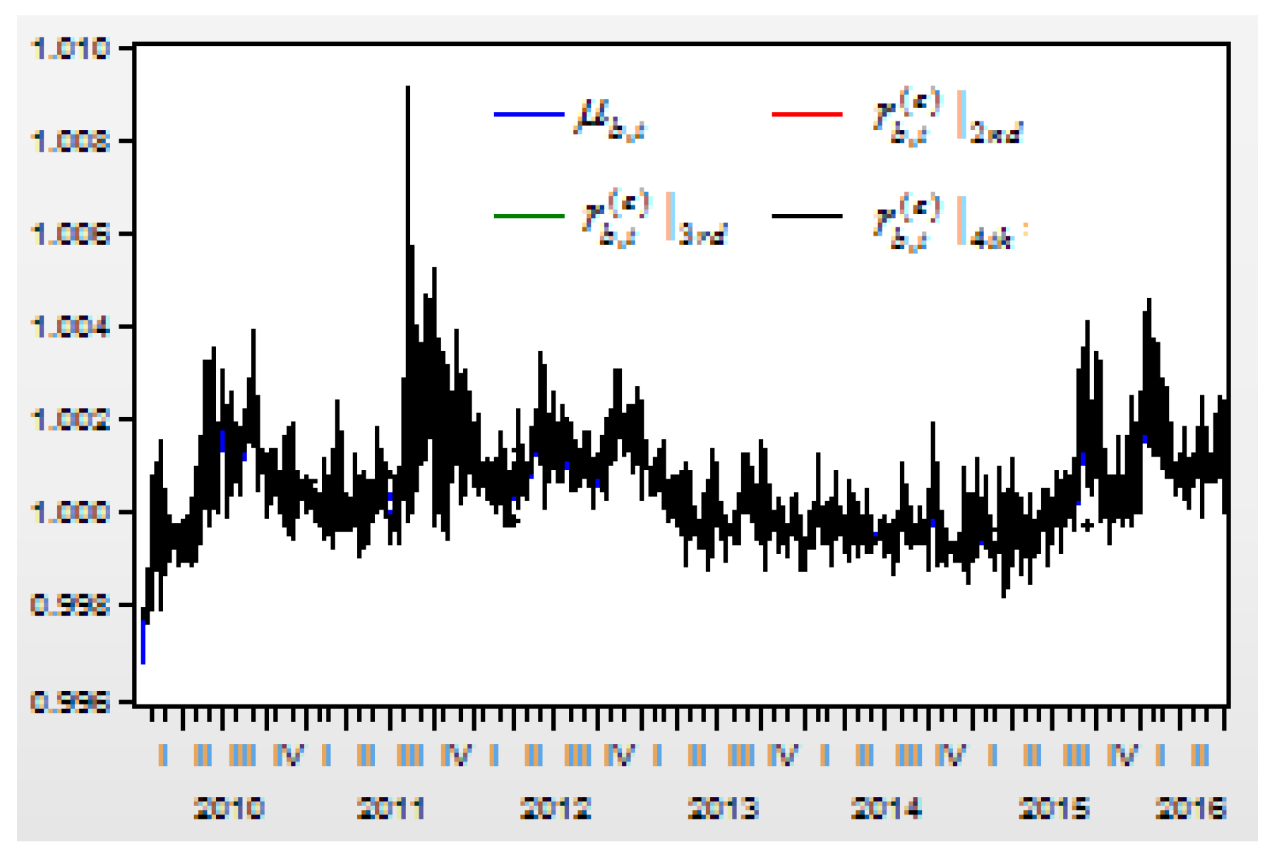
Figure 17 shows the curves of the conditional mean ${\mu }_{b,t}$ of the return index $r_t$ and the prediction values $r_{b,t}^{(2)}$, $r_{b,t}^{(3)}$, and $r_{b,t}^{(4)}$ of the return index $r_t$ from the second, third, and fourth difference probability prediction values during 2010–2016.

The correlations between $r_t$ and ${\mu }_{b,t}$, $r_{b,t}^{(2)}$, $r_{b,t}^{(3)}$, $r_{b,t}^{(4)}$ are 0.1018, 0.1614, 0.1435, 0.1614, respectively. It is obvious that the residual item $b_t$ has made the correlations between the return index $r_t$ and its prediction values, $r_{b,t}^{(2)}$, $r_{b,t}^{(3)}$, $r_{b,t}^{(4)}$ increase much more than the correlation between the return index $r_t$ and its prediction values of the conditional mean ${\mu }_{b,t}$. This means that applying the second-, third-, and fourth-order finite differences to the residual item $b_t$ can improve the correlations between the real return index $r_t$ and its prediction values.

5.5. Return Index Prediction Based on the Second-Order Difference ARDL-CRG-FD Model

Because applying the second, third, and fourth-order finite difference methods to the residual item $b_t$ can improve the correlations between the real return index $r_t$ and its prediction values, we will test if higher lags of the probability $q_t^{(b)}$ regression model can lead to a higher correlation between the real return index $r_t$ and its prediction value. For this purpose, we will focus on conducting an analysis of the second-order finite difference regression model.

The second-order difference $d^2{q}_t^{(b)}$ can be expressed by a regression model as

$$d^2{q}_t^{(b)}=\omega +{\alpha }_0{q}_{t-1}^{(b)}+{\alpha }_1{q}_{t-1}^{(b)}+{\displaystyle \sum }_{j=1}^p{\beta }_j{d}^2{q}_{t-j}^{(b)}+c_t$$

When the lag-order is $p=3,50,100,150,200,300,400,500,600,700$, we can obtain ten different prediction regression models for the second-order difference $d^2{q}_t^{(b)}$.

By applying the equations of $q_t^{(b)}=q_{t-1}^{(b)}+d{q}_{t-1}^{(b)}+d^2{q}_t^{(b)}$, $r_{b,t}^{(c)}={\mu }_{b,t}^{(c)}-\ln (\frac{1}{q_t^{(b)}}-1)$, and $r_{b,t}=r_{b,t}^{(c)}/r_{t-1}^{(c)}$, we will be able to obtain the return index prediction values of $r_{b,t}{|}_{p=3,50,150,200,300,400,500,600,700}$.

Table 7. Results of the second-order finite difference regression models of ARDL-CRG-FD when the lags of the probability are different.

No.	Prediction Model for Second-Order Difference ${\mathit{d}}^2{\mathit{q}}_{\mathit{t}}^{(\mathit{b})}$								${\mathit{r}}_{\mathit{b},\mathit{t}}$	Correlation $\rho ({\mathit{r}}_{\mathit{b},\mathit{t}},{\mathit{r}}_{\mathit{t}})$
	$\mathit{\omega }$	${\mathit{\alpha }}_0$	${\mathit{\alpha }}_1$	$\mathit{p}$	${\mathit{R}}^2$	$\mathit{S}.\mathit{E}.$	$\mathit{A}\mathit{I}\mathit{C}$	$\mathit{S}\mathit{I}\mathit{C}$
1	0.563364	−1.126737	−0.675543	3	0.842668	0.003118	−8.699228	−8.678259	$r_{b,t}{|}_{p=3}$	0.161486
2	0.538496	−1.077017	−0.410510	50	0.847195	0.003144	−8.651569	−8.461571	$r_{b,t}{|}_{p=50}$	0.242633
3	0.421591	−0.843178	−20.90050	100	0.852919	0.003136	−8.622071	−8.242382	$r_{b,t}{|}_{p=100}$	0.296988
4	0.373183	−0.746334	−35.27877	150	0.860050	0.003148	−8.579957	−7.999447	$r_{b,t}{|}_{p=150}$	0.344799
5	0.398982	−0.797960	−15.82828	200	0.863607	0.003214	−8.503039	−7.709469	$r_{b,t}{|}_{p=200}$	0.382242
6	0.343252	−0.686537	−28.55671	300	0.877231	0.003315	−8.370555	−7.108924	$r_{b,t}{|}_{p=300}$	0.478909
7	0.667269	−1.334446	199.7550	400	0.891028	0.003242	−8.352795	−6.556372	$r_{b,t}{|}_{p=400}$	0.584397
8	0.563196	−1.126326	140.5567	500	0.906935	0.003267	−8.302990	−5.888115	$r_{b,t}{|}_{p=500}$	0.656670
9	2.112864	−4.225520	1324.022	600	0.930281	0.003485	−8.230197	−5.089768	$r_{b,t}{|}_{p=600}$	0.752572
10	4.288409	−8.576220	3052.109	700	0.961514	0.004071	−8.362576	−4.355974	$r_{b,t}{|}_{p=700}$	0.873537

has listed the first three parameters of the second-order difference regression models for the residual of the cumulative return index prediction model.

When the lag order $p=3$, the regression model of the second-order difference $d^2{q}_t^{(b)}$ includes the intercept $\omega$ and the coefficient ${\alpha }_0$ for item $q_{t-1}^{(b)}$, the coefficient ${\alpha }_1$ for item $d{q}_{t-1}^{(b)}$, and the coefficient ${\beta }_1,{\beta }_2,{\beta }_3$ for item $q_{t-1}^{(b)},q_{t-2}^{(b)},q_{t-3}^{(b)}$.

When the lag order $p=50$, the regression model of the second-order difference $d^2{q}_t^{(b)}$ includes the intercept $\omega$ and the coefficient ${\alpha }_0$ for item $q_{t-1}^{(b)}$, the coefficient ${\alpha }_1$ for item $d{q}_{t-1}^{(b)}$, and the coefficient ${\beta }_1,{\beta }_2,\dots ,{\beta }_{50}$ for item $q_{t-1}^{(b)},q_{t-2}^{(b)},\dots ,q_{t-50}^{(b)}$.

Similarly, When the lag order $p=700$, the regression model of the second-order difference $d^2{q}_t^{(b)}$ includes the intercept $\omega$ and the coefficient ${\alpha }_0$ for item $q_{t-1}^{(b)}$, the coefficient ${\alpha }_1$ for item $d{q}_{t-1}^{(b)}$, and the coefficient ${\beta }_1,{\beta }_2,\dots ,{\beta }_{700}$ for item $q_{t-1}^{(b)},q_{t-2}^{(b)},\dots ,q_{t-700}^{(b)}$.

Figure 18 depicts the curves of the return index $r_t$ and its prediction values of $r_{b,t}{|}_{p=200}$ from the second-order difference regression model.

Figure 19 depicts the curves of the return index $r_t$ and its prediction values of $r_{b,t}{|}_{p=700}$ from the second-order difference regression model.

From these regression models for the second-order difference variable $d^2{q}_t^{(b)}$, there are three results:

First, when the lag order increases, the determinate coefficient for the regression model will increase. When the lag order increases from 3 to 50, 100, 150, 200, 300, 400, 500, 600, and 700, the R-squared value of the regression model increases from 0.842668 to 0.847195, 0.852919, 0.860050, 0.863607, 0.877231, 0.891028, 0.906935, 0.930281, and 0.961514, respectively.

Second, when the lag order increases, the correlations between the real return index $r_t$ and its prediction values will increase. When the lag order increases from 3 to 50, 100, 150, 200, 300, 400, 500, 600, and 700, the correlation between $r_t$ and its prediction value of $r_{b,t}{|}_{p=3}$, $r_{b,t}{|}_{p=50}$, $r_{b,t}{|}_{p=100}$, $r_{b,t}{|}_{p=150}$, $r_{b,t}{|}_{p=200}$, $r_{b,t}{|}_{p=300}$, $r_{b,t}{|}_{p=400}$, $r_{b,t}{|}_{p=500}$, $r_{b,t}{|}_{p=600}$, $r_{b,t}{|}_{p=700}$ increases from 0.161486 to 0.242633, 0.296988, 0.344799, 0.382242, 0.478909, 0.584397, 0.656670, 0.752572, and 0.873537, respectively.

Third, when comparing both figures, we can see that the prediction values of $r_{b,t}{|}_{p=700}$ are more approximated to the real return index $r_t$ than the prediction values of $r_{b,t}{|}_{p=200}$. This means that a higher lag order prediction model can create a higher approximated result between the real return index $r_t$ and its prediction value.

5.6. ARDL-CRG-GARCH-FD Model and Return Index Prediction Based on the Finite Difference Method

For the residual variable $b_t$, the conditional volatility in the GARCH (1,1) model is regressed as

$$\begin{gathered} {\sigma }_{b,t}^2=6.59E-0.6+0.134894b_{t-1}^2+0.823964{\sigma }_{b,t-1}^2 \\ LL=3276.90, AIC=-4.27, SIC=-4.26, HIC=-4.27 \end{gathered}$$

where the static variance is ${\overline{\sigma }}^2=0.01265$, the coefficient of the ARCH item is $\alpha =0.134894>0$, the coefficient of the GARCH item is $\beta =0.823964>0$, the intercept is $\omega =0.00000659>0$, and the three parameters satisfy the relation of $\alpha +\beta =0.958858<1$, $\omega +\alpha +\beta =0.95886459<1$.

Because the regressive residual is unavoidable, the mean and variance of the random variable $e_{b,t}=b_t/{\sigma }_{b,t}$ are 0.000692 and 1.005242, respectively. When the new standardized random variable is defined by $e_{b,t}=({\epsilon }_{b,t}-{\mu }_{b,0})/{\sigma }_{b,0}$, the mean and variance of the random variable $e_{b,t}$ are 1.74E-18 and 1.000327, respectively. Obviously, the random variable $e_{b,t}$ is more approximate to the standardized normal distribution than the random variable ${\epsilon }_{b,t}$.

Then, the prediction value of the cumulative return index $r_t^{(c)}$ will be

$$r_{b,t}^{(c,e)}={\mu }_{b,t}^{(c)}+{\sigma }_{b,t}(mean({\epsilon }_{b,t})+\mathrm{Var}({\epsilon }_{b,t})e_{b,t})$$

When the variable $q_{b,t}^{(e)}$ represents the probability of the quantile of $e_{b,t}$, let $q_{b,t}^{(e)}=\frac{1}{1+e^{-e_{b,t}}}$. Assume that the probability $q_{b,t}^{(e)}$ is the same as the probability of the random variable with the standard normal distribution, then for simplicity, the prediction model of the cumulative return index $r_t^{(c)}$ can be defined as

$$r_{b,t}^{(c,e)}={\mu }_{b,t}^{(c)}+{\sigma }_{b,t}(mean({\epsilon }_{b,t})+\mathrm{Var}({\epsilon }_{b,t})(-\ln (\frac{1}{q_{b,t}^{(e)}}-1)))$$

Then, the prediction model of the return index $r_t$ can be defined as

$$r_{b,t}^{(e)}=\frac{r_{b,t}^{(c,e)}}{r_{b,t}^{(c)}}$$

The probability prediction models from the second-order difference are

$$\begin{gathered} d^2{q}_{b,t}^{(e)}=0.534293-1.060669q_{b,t-1}^{(e)}-0.820323d{q}_{b,t-1}^{(e)}-0.152446d^2{q}_{b,t-1}^{(e)}-0.102566d^2{q}_{b,t-2}^{(e)}-0.052680d^2{q}_{b,t-3}^{(e)} \\ {R}^2=0.9532, S.E.=0.2014,AIC=-0.3625, SIC=-0.3415 \\ {q}_{b,t}^{(e)}=q_{b,t-1}^{(e)}+d{q}_{b,t-1}^{(e)}+d^2{q}_{b,t}^{(e)} \end{gathered}$$

The probability prediction models from the third-order difference are

$$\begin{gathered} q_{b,t}^{(e)}=0.534293-1.060669q_{b,t-1}^{(e)}-0.820323d{q}_{b,t-1}^{(e)}-1.307692d^2{q}_{b,t-1}^{(e)}+0.155246d^3{q}_{b,t-1}^{(e)}-0.052680d^3{q}_{b,t-2}^{(e)} \\ {R}^2=0.9532, S.E.=0.2014,AIC=-0.3625, SIC=-0.3415 \\ {q}_{b,t}^{(e)}=q_{b,t-1}^{(e)}+d{q}_{b,t-1}^{(e)}+d^2{q}_{b,t-1}^{(e)}+d^3{q}_{b,t}^{(e)} \end{gathered}$$

The probability prediction models from the fourth-order difference are

$$\begin{gathered} d^4{q}_{b,t}^{(e)}=0.534293-1.060669q_{b,t-1}^{(e)}-0.820323d{q}_{b,t-1}^{(e)}-1.307692d^2{q}_{b,t-1}^{(e)}-0.792074d^3{q}_{b,t-1}^{(e)}-0.052680d^4{q}_{b,t-1}^{(e)} \\ {R}^2=0.9867, S.E.=0.2014,AIC=-0.3625, SIC=-0.3415 \\ {q}_{b,t}^{(e)}=q_{b,t-1}^{(e)}+d{q}_{b,t-1}^{(e)}+d^2{q}_{b,t-1}^{(e)}+d^3{q}_{b,t-1}^{(e)}+d^4{q}_{b,t}^{(e)} \end{gathered}$$

Assume variable $r_{b,t}^{(e)}{|}_{2nd}$ represents the prediction value of the return index $r_t$ from the second-order difference probability prediction value of $q_{b,t}^{(e)}$; variable $r_{b,t}^{(e)}{|}_{3rd}$ represents the prediction value of the return index $r_t$ from the third-order difference probability prediction value of $q_{b,t}^{(e)}$; and variable $r_{b,t}^{(e)}{|}_{4th}$ represents the prediction value of the return index $r_t$ from the fourth-order difference probability prediction value of $q_{b,t}^{(e)}$.

Figure 20 shows the curves of the return index $r_t$ and its prediction values of $r_{b,t}^{(e)}{|}_{2nd}$, $r_{b,t}^{(e)}{|}_{3rd}$, and $r_{b,t}^{(e)}{|}_{4th}$ from the second, third, and fourth difference probability prediction values during 2010–2016.

Figure 21 shows the curves of the conditional mean ${\mu }_{b,t}$ of the return index $r_t$ and the prediction values $r_{b,t}^{(e)}{|}_{2nd}$, $r_{b,t}^{(e)}{|}_{3rd}$, and $r_{b,t}^{(e)}{|}_{4th}$ of the return index $r_t$ from the second, third, and fourth order difference probability prediction values during 2010–2016.

The correlations between $r_t$ and ${\mu }_{b,t}$, $r_{b,t}^{(e)}{|}_{2nd}$, $r_{b,t}^{(e)}{|}_{3rd}$, and $r_{b,t}^{(e)}{|}_{4th}$ are 0.1006, 0.1467, 0.1467, 0.1467, respectively. It is obvious that the residual item $b_t$ has made the correlations between the return index $r_t$ and its prediction values $r_{b,t}^{(e)}{|}_{2nd}$, $r_{b,t}^{(e)}{|}_{3rd}$, and $r_{b,t}^{(e)}{|}_{4th}$ increase much more than the correlation between the return index $r_t$ and its prediction values of the conditional mean ${\mu }_{b,t}$.

5.7. Return Index Prediction Based on the Second-Order Difference ARDL-CRG-GARCH-FD Model

Because applying the second-, third-, and fourth-order finite difference methods to the residual item $e_{b,t}$ can improve the correlations between the real return index $r_t$ and its prediction values, we will test if higher lags of the probability prediction value of the $q_{b,t}^{(e)}$ regression model can lead to a higher correlation between the real return index $r_t$ and its prediction value. For this purpose, we will focus on conducting an analysis of the second-order finite difference regression model.

The second-order difference $d^2{q}_{b,t}^{(e)}$ can be expressed by a regression model as

$$d^2{q}_{b,t}^{(e)}=\omega +{\alpha }_0{q}_{b,t-1}^{(e)}+{\alpha }_{1}d{q}_{b,t-1}^{(e)}+{\displaystyle \sum }_{j=1}^p{\beta }_j{d}^2{q}_{b,t-j}^{(e)}+c_t$$

When the lag order is $p=3,50,100,150,200,300,400,500,600,700$, we can obtain ten different prediction regression models for the second-order difference $d^2{q}_{b,t}^{(e)}$.

According to the second-order difference equation $q_{b,t}^{(e)}=q_{b,t-1}^{(e)}+d{q}_{b,t-1}^{(e)}+d^2{q}_{b,t}^{(e)}$, the return index prediction regression model $r_{b,t}^{(c,e)}={\mu }_{b,t}^{(c)}+{\sigma }_{b,t}(mean({\epsilon }_{b,t})+\mathrm{Var}r({\epsilon }_{b,t})(-\ln (1/q_{b,t}^{(e)}-1)))$, and the return index prediction model $r_{b,t}^{(e)}=r_{b,t}^{(c,e)}/r_{b,t}^{(c)}$, we will be able to obtain the return index prediction values of $r_{b,t}^{(e)}{|}_{p=3,50,100,150,200,300,400,500,600,700}$.

Table 8. Results of the second-order finite difference ARDL-CRG-GARCH-FD models when the lags of the probability are different.

No.	Prediction Model for Second-Order Difference ${\mathit{d}}^2{\mathit{q}}_{\mathit{b},\mathit{t}}^{(\mathit{e})}$								${\mathit{r}}_{\mathit{b},\mathit{t}}^{(\mathit{e})}$	Correlation $\rho ({\mathit{r}}_{\mathit{b},\mathit{t}}^{(\mathit{e})},{\mathit{r}}_{\mathit{t}})$
	$\mathit{\omega }$	${\mathit{\alpha }}_0$	${\mathit{\alpha }}_1$	$\mathit{p}$	${\mathit{R}}^2$	$\mathit{S}.\mathit{E}.$	$\mathit{A}\mathit{I}\mathit{C}$	$\mathit{S}\mathit{I}\mathit{C}$
1	0.534293	−1.060669	−0.820323	3	0.842384	0.201461	−0.362523	−0.341564	$r_{b,t}^{(e)}{|}_{p=3}$	0.146718
2	0.442926	−0.881374	−6.802927	50	0.845745	0.202992	−0.316119	−0.126225	$r_{b,t}^{(e)}{|}_{p=50}$	0.220724
3	0.364174	−0.723608	−19.37262	100	0.852091	0.202484	−0.286966	0.092508	$r_{b,t}^{(e)}{|}_{p=100}$	0.284660
4	0.300778	−0.596242	−37.47253	150	0.857610	0.204075	−0.236363	0.343807	$r_{b,t}^{(e)}{|}_{p=150}$	0.329443
5	0.330035	−0.655289	−19.05648	200	0.861082	0.206740	−0.174969	0.618118	$r_{b,t}^{(e)}{|}_{p=200}$	0.368404
6	0.331949	−0.659683	1.016989	300	0.875154	0.210358	−0.070013	1.190792	$r_{b,t}^{(e)}{|}_{p=300}$	0.472701
7	0.589264	−1.164536	161.4154	400	0.892694	0.210504	−0.006255	1.788893	$r_{b,t}^{(e)}{|}_{p=400}$	0.566134
8	0.504847	−0.998953	135.5047	500	0.910258	0.214921	0.069515	2.482519	$r_{b,t}^{(e)}{|}_{p=500}$	0.646393
9	2.024880	−3.998776	1122.926	600	0.933839	0.224660	0.102500	3.240248	$r_{b,t}^{(e)}{|}_{p=600}$	0.732672
10	3.727738	−7.356259	2310.739	700	0.965393	0.250051	−0.122220	3.880572	$r_{b,t}^{(e)}{|}_{p=700}$	0.840273

has listed the first three parameters of the second-order finite difference regression models for the residual of the cumulative return index prediction model.

When the lag order $p=3$, the regression model of the second-order difference $d^2{q}_t^{(b)}$ includes the intercept $\omega$ and the coefficient ${\alpha }_0$ for item $q_{t-1}^{(b)}$, the coefficient ${\alpha }_1$ for item $d{q}_{t-1}^{(b)}$, and the coefficient ${\beta }_1,{\beta }_2,{\beta }_3$ for item $q_{t-1}^{(b)},q_{t-2}^{(b)},q_{t-3}^{(b)}$.

When the lag order $p=50$, the regression model of the second-order difference $d^2{q}_t^{(b)}$ includes the intercept $\omega$ and the coefficient ${\alpha }_0$ for item $q_{t-1}^{(b)}$, the coefficient ${\alpha }_1$ for item $d{q}_{t-1}^{(b)}$, and the coefficient ${\beta }_1,{\beta }_2,\dots ,{\beta }_{50}$ for item $q_{t-1}^{(b)},q_{t-2}^{(b)},\dots ,q_{t-50}^{(b)}$.

Similarly, when the lag order $p=700$, the regression model of the second-order difference $d^2{q}_t^{(b)}$ includes the intercept $\omega$ and the coefficient ${\alpha }_0$ for item $q_{t-1}^{(b)}$, the coefficient ${\alpha }_1$ for item $d{q}_{t-1}^{(b)}$, and the coefficient ${\beta }_1,{\beta }_2,\dots ,{\beta }_{700}$ for item $q_{t-1}^{(b)},q_{t-2}^{(b)},\dots ,q_{t-700}^{(b)}$.

Figure 22 depicts the curves of the return index $r_t$ and its prediction values of $r_{b,t}^{(e)}{|}_{p=200}$ from the second-order finite difference regression model.

Figure 23 depicts the curves of the return index $r_t$ and its prediction values of $r_{b,t}^{(e)}{|}_{p=700}$ from the second-order finite difference regression model.

From these regression models for the second-order difference variable $d^2{q}_t^{(b)}$, there are three results:

First, when the lag order increases, the determinate coefficient for the regression model will increase. When the lag order increases from 3 to 50, 100, 150, 200, 300, 400, 500, 600, and 700, the R-squared value of the regression model increases from 0.842384 to 0.845745, 0.852091, 0.857610, 0.861082, 0.875154, 0.892694, 0.910258, 0.933839, and 0.965393, respectively.

Second, when the lag order increases, the correlations between the real return index $r_t$ and its prediction values will increase. When the lag order increases from 3 to 50, 100, 150, 200, 300, 400, 500, 600, and 700, the correlation between $r_t$ and its prediction values of $r_{b,t}^{(e)}{|}_{p=3}$, $r_{b,t}^{(e)}{|}_{p=50}$, $r_{b,t}^{(e)}{|}_{p=100}$, $r_{b,t}^{(e)}{|}_{p=150}$, $r_{b,t}^{(e)}{|}_{p=200}$, $r_{b,t}^{(e)}{|}_{p=300}$, $r_{b,t}^{(e)}{|}_{p=400}$, $r_{b,t}^{(e)}{|}_{p=500}$, $r_{b,t}^{(e)}{|}_{p=600}$, $r_{b,t}^{(e)}{|}_{p=700}$ increases from 0.146718 to 0.220724, 0.284660, 0.329443, 0.368404, 0.472701, 0.566134, 0.646393, 0.732672, and 0.840273, respectively.

Third, when we compare both figures, we can see that the prediction values of $r_{b,t}^{(e)}{|}_{p=700}$ are more approximated to the real return index $r_t$ than the prediction values of $r_{b,t}^{(e)}{|}_{p=200}$. This means that a higher lag order of the probability $r_{b,t}^{(e)}$ prediction model can create a higher approximated result between the real return index $r_t$ and its prediction value.

6. Tests of the Prediction Accuracy for the Four Kinds of Models

6.1. Comparison of the Correlations between the Real and Predicted Returns from the Four Different Models

From the probability prediction models, we have already learned that the correlations between the real return index $r_t$ and its prediction values from the higher order differences are higher than the correlations between the real return index $r_t$ and its prediction values from the lower order differences.

When we fixed the finite difference order of the probability variable $q_t$ that transferred from the residual variable $a_t$ at the second order, the higher lags of the probability variable $q_t$ will make higher correlations between the real return index $r_t$ and its prediction values for each of the four different prediction models.

It is clear that the higher correlations mean that the prediction accuracy is high. For the four different models, we will compare the empirical results based on the perspectives of the correlations.

From the previous study, we built an AR(5) model when the lag order is $p=5$ and the lag items are $r_{t-1},r_{t-2},r_{t-3},r_{t-4},r_{t-5}$ from the real return index $r_t$. We also built an ARDL-CRG model when the cumulative gap lag order is 1 as item $r_{t-1}^{(c,gap)}$. Based on the two models’ residual items, by using a second-order finite difference method, we have already built four different models.

Table 9. Correlations between the real return index and its prediction values from four different kinds of prediction models.

$r_{a,t}$	$\mathsf{\rho }(r_{a,t},r_t)$	$r_{b,t}$	$\mathsf{\rho }(r_{b,t},r_t)$	$r_{a,t}^{(e)}$	$\mathsf{\rho }(r_{a,t}^{(e)},r_t)$	$r_{b,t}^{(e)}$	$\mathsf{\rho }(r_{b,t}^{(e)},r_t)$
$r_{a,t}{|}_{p=3}$	0.136766	$r_{b,t}{|}_{p=3}$	0.161486	$r_{a,t}^{(e)}{|}_{p=3}$	0.119018	$r_{b,t}^{(e)}{|}_{p=3}$	0.146718
$r_{a,t}{|}_{p=50}$	0.238128	$r_{b,t}{|}_{p=50}$	0.242633	$r_{a,t}^{(e)}{|}_{p=50}$	0.209055	$r_{b,t}^{(e)}{|}_{p=50}$	0.220724
$r_{a,t}{|}_{p=100}$	0.294749	$r_{b,t}{|}_{p=100}$	0.296988	$r_{a,t}^{(e)}{|}_{p=100}$	0.268237	$r_{b,t}^{(e)}{|}_{p=100}$	0.284660
$r_{a,t}{|}_{p=150}$	0.341969	$r_{b,t}{|}_{p=150}$	0.344799	$r_{a,t}^{(e)}{|}_{p=150}$	0.315291	$r_{b,t}^{(e)}{|}_{p=150}$	0.329443
$r_{a,t}{|}_{p=200}$	0.389903	$r_{b,t}{|}_{p=200}$	0.382242	$r_{a,t}^{(e)}{|}_{p=200}$	0.367438	$r_{b,t}^{(e)}{|}_{p=200}$	0.368404
$r_{a,t}{|}_{p=300}$	0.486086	$r_{b,t}{|}_{p=300}$	0.478909	$r_{a,t}^{(e)}{|}_{p=300}$	0.472224	$r_{b,t}^{(e)}{|}_{p=300}$	0.472701
$r_{a,t}{|}_{p=400}$	0.578318	$r_{b,t}{|}_{p=400}$	0.584397	$r_{a,t}^{(e)}{|}_{p=400}$	0.552860	$r_{b,t}^{(e)}{|}_{p=400}$	0.566134
$r_{a,t}{|}_{p=500}$	0.651674	$r_{b,t}{|}_{p=500}$	0.656670	$r_{a,t}^{(e)}{|}_{p=500}$	0.640771	$r_{b,t}^{(e)}{|}_{p=500}$	0.646393
$r_{a,t}{|}_{p=600}$	0.745966	$r_{b,t}{|}_{p=600}$	0.752572	$r_{a,t}^{(e)}{|}_{p=600}$	0.701112	$r_{b,t}^{(e)}{|}_{p=600}$	0.732672
$r_{a,t}{|}_{p=700}$	0.867847	$r_{b,t}{|}_{p=700}$	0.873537	$r_{a,t}^{(e)}{|}_{p=700}$	0.847974	$r_{b,t}^{(e)}{|}_{p=700}$	0.840273

has listed the correlations between the real return index $r_t$ and its prediction values of $r_{a,t}$, $r_{b,t}$, $r_{a,t}^{(e)}$, and $r_{a,t}^{(e)}$ from the four different kinds of prediction models.

First, the perspective of AR-FD models is considered. The prediction values of $r_{a,t}$ are from the traditional autoregressive (AR) model $r_{a,t}={\mu }_{a,t}+a_t$. When the probability is defined as $q_t^{(a)}=1/(1+e^{-a_t})$, the residual item $a_t=-\ln (1/q_t^{(a)}-1)$ can be predicted by predicting the probability $q_t^{(a)}$. Because the second-order difference $d^2{q}_t^{(a)}$ of the probability $q_t^{(a)}$ is an autoregressive time series, the probability $q_t^{(a)}$ can be predicted by predicting its second-order difference $d^2{q}_t^{(a)}$. When we choose different lag orders for the second-order difference $d^2{q}_t^{(a)}$ as $d^2{q}_{t-3}^{(a)}$, $d^2{q}_{t-50}^{(a)}$, …, and $d^2{q}_{t-700}^{(a)}$, we will obtain the prediction values of $r_{a,t}{|}_{p=3}$, $r_{a,t}{|}_{p=50}$, …, and $r_{a,t}{|}_{p=700}$. When the lag order increases, the correlation between the real return index $r_t$ and the prediction values of $r_{a,t}$ will increase.

Second, from the perspective of ARDL-CRG-FD models, the prediction values of $r_{b,t}$ are from the traditional autoregressive distribution lag (ARDL) model $r_{b,t}^{(c)}={\mu }_{b,t}^{(c)}+b_t$. Because $r_{b,t}=r_{b,t}^{(c)}/r_{t-1}^{(c)}$, it is easy to predict the values of the return index if we know the prediction values of the cumulative return index. When the probability is defined as $q_t^{(b)}=1/(1+e^{-b_t})$, then the residual item $b_t=-\ln (1/q_t^{(b)}-1)$ can be predicted by predicting the probability $q_t^{(b)}$. Because the second-order difference $d^2{q}_t^{(b)}$ of the probability $q_t^{(b)}$ is an autoregressive time series, the probability $q_t^{(b)}$ can be predicted by predicting its second-order difference $d^2{q}_t^{(b)}$. When we choose different lag orders for the second-order difference $d^2{q}_t^{(b)}$ as $d^2{q}_{t-3}^{(b)}$, $d^2{q}_{t-50}^{(b)}$, …, and $d^2{q}_{t-700}^{(b)}$, we will get the prediction values of $r_{b,t}{|}_{p=3}$, $r_{b,t}{|}_{p=50}$, …, and $r_{b,t}{|}_{p=700}$. When the lag order increases, the correlation between the real return index $r_t$ and the prediction values of $r_{b,t}$ will increase.

Third, from the perspective of AR-GARCH-FD models, the prediction values of $r_{a,t}^{(e)}$ are from the traditional autoregressive (AR) model and the generalized autoregressive conditional heteroscedasticity (GARCH) model $r_{a,t}={\mu }_{a,t}+a_t$, $a_t={\sigma }_{a,t}{\epsilon }_{a,t}$, ${\epsilon }_{a,t}=a_t/{\sigma }_{a,t}$, $e_{a,t}=({\epsilon }_{a,t}-{\mu }_{a,0})/{\sigma }_{a,0}$. When the probability is defined as $q_{a,t}^{(e)}=1/(1+e^{-e_{a,t}})$, by predicting the probability $q_{a,t}^{(e)}$, the residual item $a_t={\sigma }_{a,t}({\mu }_{a,0}+{\sigma }_{a,0}(-\ln (1/q_{a,t}^{(e)}-1)))$ can be predicted. Because the second-order difference $d^2{q}_{a,t}^{(e)}$ of the probability $q_{a,t}^{(e)}$ is an autoregressive time series, the probability $q_{a,t}^{(e)}$ can be predicted by predicting its second-order difference $d^2{q}_{a,t}^{(e)}$. When we choose different lag orders for the second-order difference $d^2{q}_{a,t}^{(e)}$ as $d^2{q}_{a,t-3}^{(e)}$, $d^2{q}_{a,t-50}^{(e)}$, …, and $d^2{q}_{a,t-700}^{(e)}$, we will get the prediction values of $r_{a,t}^{(e)}{|}_{p=3}$, $r_{a,t}^{(e)}{|}_{p=50}$, …, and $r_{a,t}^{(e)}{|}_{p=700}$. When the lag order increases, the correlation between the real return index $r_t$ and the prediction values of $r_{a,t}^{(e)}$ will increase.

Fourth, from the perspective of ARDL-CRG-GARCH-FD models, the prediction values of $r_{b,t}^{(e)}$ are from the traditional autoregressive distribution lag (ARDL) model and the generalized autoregressive conditional heteroscedasticity (GARCH) model $r_{b,t}^{(c)}={\mu }_{b,t}^{(c)}+b_t$, $b_t={\sigma }_{b,t}{\epsilon }_{b,t}$, ${\epsilon }_{b,t}=b_t/{\sigma }_{b,t}$, $e_{b,t}=({\epsilon }_{b,t}-{\mu }_{b,0})/{\sigma }_{b,0}$. When the probability is defined as $q_{b,t}^{(e)}=1/(1+e^{-e_{b,t}})$, by predicting the probability $q_{b,t}^{(e)}$, the residual item $b_t={\sigma }_{b,t}(mean({\epsilon }_{b,t})+\mathrm{Var}({\epsilon }_{b,t})(-\ln (1/q_{b,t}^{(e)}-1)))$ can be predicted. Because the second-order difference $d^2{q}_{b,t}^{(e)}$ of the probability $q_{b,t}^{(e)}$ is an autoregressive time series, the probability $q_{b,t}^{(e)}$ can be predicted by predicting its second-order difference $d^2{q}_{b,t}^{(e)}$. When we choose different lag orders for the second-order difference $d^2{q}_{b,t}^{(e)}$ as $d^2{q}_{b,t-3}^{(e)}$, $d^2{q}_{b,t-50}^{(e)}$, …, and $d^2{q}_{b,t-700}^{(e)}$, we will get the prediction values of $r_{b,t}^{(e)}{|}_{p=3}$, $r_{b,t}^{(e)}{|}_{p=50}$, …, and $r_{b,t}^{(e)}{|}_{p=700}$. When the lag order increases, the correlation between the real return index $r_t$ and the prediction values of $r_{b,t}^{(e)}$ will increase.

Table 10. Comparison of correlations between the return index and the prediction values from AR, ARDL, AR-GARCH, ARDL-GARCH.

$\mathbf{\rho }({\mathit{r}}_{\mathit{a},\mathit{t}},{\mathit{r}}_{\mathit{t}})$	$\mathbf{\rho }({\mathit{r}}_{\mathit{b},\mathit{t}},{\mathit{r}}_{\mathit{t}})$	$\mathbf{\rho }({\mathit{r}}_{\mathit{a},\mathit{t}}^{(\mathit{e})},{\mathit{r}}_{\mathit{t}})$	$\mathbf{\rho }({\mathit{r}}_{\mathit{b},\mathit{t}}^{(\mathit{e})},{\mathit{r}}_{\mathit{t}})$	Correlation	Correlation	Correlation	Correlation
(1)	(2)	(3)	(4)	(2)–(1)	(4)–(3)	(1)–(3)	(2)–(4)
$r_{a,t}{|}_{p=3}$	$r_{b,t}{|}_{p=3}$	$r_{a,t}^{(e)}{|}_{p=3}$	$r_{b,t}^{(e)}{|}_{p=3}$	0.024720	0.027700	0.017748	0.014768
$r_{a,t}{|}_{p=50}$	$r_{b,t}{|}_{p=50}$	$r_{a,t}^{(e)}{|}_{p=50}$	$r_{b,t}^{(e)}{|}_{p=50}$	0.004505	0.011669	0.029073	0.021909
$r_{a,t}{|}_{p=100}$	$r_{b,t}{|}_{p=100}$	$r_{a,t}^{(e)}{|}_{p=100}$.	$r_{b,t}^{(e)}{|}_{p=100}$	0.002239	0.016423	0.026512	0.012328
$r_{a,t}{|}_{p=150}$	$r_{b,t}{|}_{p=150}$	$r_{a,t}^{(e)}{|}_{p=150}$	$r_{b,t}^{(e)}{|}_{p=150}$	0.002830	0.014152	0.026678	0.015356
$r_{a,t}{|}_{p=200}$	$r_{b,t}{|}_{p=200}$	$r_{a,t}^{(e)}{|}_{p=200}$	$r_{b,t}^{(e)}{|}_{p=200}$	−0.007661	0.000966	0.022465	0.013838
$r_{a,t}{|}_{p=300}$	$r_{b,t}{|}_{p=300}$	$r_{a,t}^{(e)}{|}_{p=300}$	$r_{b,t}^{(e)}{|}_{p=300}$	−0.007177	0.000477	0.013862	0.006208
$r_{a,t}{|}_{p=400}$.	$r_{b,t}{|}_{p=400}$	$r_{a,t}^{(e)}{|}_{p=400}$	$r_{b,t}^{(e)}{|}_{p=400}$	0.006079	0.013274	0.025458	0.018263
$r_{a,t}{|}_{p=500}$	$r_{b,t}{|}_{p=500}$	$r_{a,t}^{(e)}{|}_{p=500}$	$r_{b,t}^{(e)}{|}_{p=500}$.	0.004996	0.005622	0.010903	0.010277
$r_{a,t}{|}_{p=600}$	$r_{b,t}{|}_{p=600}$	$r_{a,t}^{(e)}{|}_{p=600}$	$r_{b,t}^{(e)}{|}_{p=600}$	0.006606	0.031560	0.044854	0.019900
$r_{a,t}{|}_{p=700}$.	$r_{b,t}{|}_{p=700}$	$r_{a,t}^{(e)}{|}_{p=700}$	$r_{b,t}^{(e)}{|}_{p=700}$	0.005690	−0.007701	0.019873	0.033264

lists the comparison values of the correlations between the return index and the prediction values from the AR, ARDL, AR-GARCH, and ARDL-GARCH models.

From the comparative results, we can get the following four results:

Firstly, the comparison between the correlations of $\mathsf{\rho }(r_{b,t},r_t)$ and $\mathsf{\rho }(r_{a,t},r_t)$ shows that the correlations of $\mathsf{\rho }(r_{b,t},r_t)$ are mostly greater than the correlations of $\mathsf{\rho }(r_{a,t},r_t)$. It means that the correlations between the return index $r_t$ and the prediction values $r_{b,t}$. from the ARDL-CRG-FD models for the cumulative return index are greater than the correlations between the return index $r_t$ and the prediction values $r_{a,t}$ from the AR-FD models for the return index. It reveals that the CRG model can improve the prediction accuracy.

Secondly, the comparison between the correlations of $\mathsf{\rho }(r_{b,t}^{(e)},r_t)$ and $\mathsf{\rho }(r_{a,t}^{(e)},r_t)$ shows that the correlations of $\mathsf{\rho }(r_{b,t}^{(e)},r_t)$ are mostly greater than the correlations of $\mathsf{\rho }(r_{a,t}^{(e)},r_t)$. It means that the correlations between the return index $r_t$ and the prediction values $r_{b,t}^{(e)}$ from the ARDL-CRG-GARCH-FD models for the cumulative return index are greater than the correlations between the return index $r_t$ and the prediction values $r_{a,t}^{(e)}$ from the AR-GARCH-FD models for the return index. It reveals that the CRG model can improve the prediction accuracy.

Thirdly, the comparison between the correlations of $\mathsf{\rho }(r_{a,t},r_t)$ and $\mathsf{\rho }(r_{a,t}^{(e)},r_t)$ shows that the correlations of $\mathsf{\rho }(r_{a,t},r_t)$ are greater than the correlations of $\mathsf{\rho }(r_{a,t}^{(e)},r_t)$. It means that the correlations between the return index $r_t$ and the prediction values $r_{a,t}$ from the AR-FD models for the return index are greater than the correlations between the return index $r_t$ and the prediction values $r_{a,t}^{(e)}$ from the AR-GARCH-FD models for the return index. It means that the GARCH model has little impact on prediction values.

Fourthly, the comparison between the correlations of $\mathsf{\rho }(r_{b,t},r_t)$ and $\mathsf{\rho }(r_{b,t}^{(e)},r_t)$ shows that the correlations of $\mathsf{\rho }(r_{b,t},r_t)$ are greater than the correlations of $\mathsf{\rho }(r_{b,t}^{(e)},r_t)$. It means that the correlations between the return index $r_t$ and the prediction values $r_{b,t}$ from the ARDL-CRG-FD models for the cumulative return index are greater than the correlations between the return index $r_t$ and the prediction values $r_{b,t}^{(e)}$ from the ARDL-CRG-GARCH-FD models for the cumulative return index. It means that the GARCH model has little impact on prediction values.

6.2. Hit Ratio Tests

Hit ratio analysis includes four cases: both the return index and the prediction value are upward, both the return index and the prediction value are downward, the return index is up but the prediction value is down, and the return index is down but the prediction value is up.

The ideal prediction values are that the higher hit ratios are better under the two cases when both the return index and the prediction values move upward or downward together, or the lower hit ratios are better in the two cases in both the return index and the prediction values are moving in the inverse directions.

First, the hit ratios from the AR-FD models were analyzed.

Table 11. Hit ratios between the real return index and its prediction values of the direct AR-FD model for the return index.

Condition	$\left\{{\mathit{r}}_{\mathit{t}}\ge 1\right\}{{\displaystyle \cap }}^{\text{}}\left\{\mathit{\chi }\ge 1\right\}$		$\left\{{\mathit{r}}_{\mathit{t}}\ge 1\right\}{{\displaystyle \cap }}^{\text{}}\left\{\mathit{\chi }<1\right\}$		$\left\{{\mathit{r}}_{\mathit{t}}<1\right\}{{\displaystyle \cap }}^{\text{}}\left\{\mathit{\chi }<1\right\}$		$\left\{{\mathit{r}}_{\mathit{t}}<1\right\}{{\displaystyle \cap }}^{\text{}}\left\{\mathit{\chi }\ge 1\right\}$		Total Ratio		Prediction
Hit Ratio	(1)		(2)		(3)		(4)		(1) + (3)		Windows
${\mu }_{a,t}$	540	35.39%	285	18.68%	266	17.43%	435	28.51%	806	52.82%	1526
$r_{a,t}{|}_{p=3}$	536	35.24%	286	18.80%	267	17.55%	432	28.40%	803	52.79%	1521
$r_{a,t}{|}_{p=50}$	481	32.63%	312	21.17%	324	21.98%	357	24.22%	805	54.61%	1474
$r_{a,t}{|}_{p=100}$	461	32.37%	304	21.35%	321	22.54%	338	23.74%	782	54.92%	1424
$r_{a,t}{|}_{p=150}$	455	33.11%	289	21.03%	326	23.73%	304	22.13%	781	56.84%	1374
$r_{a,t}{|}_{p=200}$	440	33.23%	270	20.39%	331	25.00%	283	21.37%	771	58.23%	1324
$r_{a,t}{|}_{p=300}$	415	33.91%	238	19.44%	354	28.92%	217	17.73%	769	62.83%	1224
$r_{a,t}{|}_{p=400}$	413	36.74%	190	16.90%	326	29.00%	195	17.35%	739	65.75%	1124
$r_{a,t}{|}_{p=500}$	379	37.01%	168	16.41%	319	31.15%	158	15.43%	698	68.16%	1024
$r_{a,t}{|}_{p=600}$	365	39.50%	137	14.83%	294	31.82%	128	13.85%	659	71.32%	924
$r_{a,t}{|}_{p=700}$	357	43.33%	94	11.41%	292	35.44%	81	9.83%	649	78.76%	824

Note: (1) variable $\chi$ represents each of the variables ${\mu }_{a,t}$, $r_{a,t}{|}_{p=3}$, …, and $r_{a,t}{|}_{p=700}$; (2) because the lag order levels in the different autoregressive models are different, the sample sizes are different.

lists the hit ratios between the real return index $r_t$ and its prediction values of $r_{a,t}$ from the direct AR-FD model for the return index at ten levels of different lag orders.

Under the ideal prediction criteria, it is clear that a higher level of lag order leads to a higher hit ratio than a lower level of lag order when both the return index and the prediction values move upward or downward together.

Secondly, the hit ratios from the ARDL-CRG-FD models were analyzed.

Table 12. Hit ratios between the return index and its prediction values of the indirect ARDL-CRG-FD model for the cumulative return index.

Condition	$\left\{{\mathit{r}}_{\mathit{t}}\ge 1\right\}{{\displaystyle \cap }}^{\text{}}\left\{\mathit{\chi }\ge 1\right\}$		$\left\{{\mathit{r}}_{\mathit{t}}\ge 1\right\}{{\displaystyle \cap }}^{\text{}}\left\{\mathit{\chi }<1\right\}$		$\left\{{\mathit{r}}_{\mathit{t}}<1\right\}{{\displaystyle \cap }}^{\text{}}\left\{\mathit{\chi }<1\right\}$		$\left\{{\mathit{r}}_{\mathit{t}}<1\right\}{{\displaystyle \cap }}^{\text{}}\left\{\mathit{\chi }\ge 1\right\}$		Total Ratio		Prediction
Hit Ratio	(1)		(2)		(3)		(4)		(1) + (3)		Windows
${\mu }_{b,t}$	510	33.33%	318	20.78%	275	17.97%	427	27.91%	785	51.31%	1530
$r_{b,t}{|}_{p=3}$	491	32.20%	333	21.84%	293	19.21%	408	26.75%	784	51.41%	1525
$r_{b,t}{|}_{p=50}$	471	31.87%	325	21.99%	336	22.73%	346	23.41%	807	54.60%	1478
$r_{b,t}{|}_{p=100}$	466	32.63%	303	21.22%	340	23.81%	319	22.34%	806	56.44%	1428
$r_{b,t}{|}_{p=150}$	455	33.02%	291	21.12%	354	25.69%	278	20.17%	809	58.71%	1378
$r_{b,t}{|}_{p=200}$	432	32.53%	280	21.08%	345	25.98%	271	20.41%	777	58.51%	1328
$r_{b,t}{|}_{p=300}$	411	33.47%	245	19.95%	351	28.58%	221	18.00%	762	62.05%	1228
$r_{b,t}{|}_{p=400}$	405	35.90%	199	17.64%	339	30.05%	185	16.40%	744	65.96%	1128
$r_{b,t}{|}_{p=500}$	380	36.96%	169	16.44%	328	31.91%	151	14.69%	708	68.87%	1028
$r_{b,t}{|}_{p=600}$	369	39.76%	133	14.33%	301	32.44%	125	13.47%	670	72.20%	928
$r_{b,t}{|}_{p=700}$	362	43.72%	91	10.99%	298	35.99%	77	9.30%	660	79.71%	828

Note: (1) variable $\chi$ represents each of the variables ${\mu }_{b,t}$, $r_{b,t}{|}_{p=3}$, …, and $r_{b,t}{|}_{p=700}$; (2) because the lag order levels in the different autoregressive models are different, the sample sizes are different.

lists the hit ratios between the real return index $r_t$ and its prediction values of $r_{b,t}$ from the indirect ARDL-CRG-FD model for the return index at ten levels of different lag orders.

Under the ideal prediction criteria, it is clear that a higher level of lag order has led to a higher hit ratio than a lower level of lag order when both the return index and the prediction values move upward or downward together.

Third, we carried out a comparison between the hit ratios from the ARDL-CRG-FD models and from the AR-FD models.

Table 13. Comparison of hit ratios between the results from the AR-FD models and the ARDL-CRG-FD models.

Condition	$\left\{{\mathit{r}}_{\mathit{t}}\ge 1\right\}{{\displaystyle \cap }}^{\text{}}\left\{\mathit{\chi }\ge 1\right\}$	$\left\{{\mathit{r}}_{\mathit{t}}\ge 1\right\}{{\displaystyle \cap }}^{\text{}}\left\{\mathit{\chi }<1\right\}$	$\left\{{\mathit{r}}_{\mathit{t}}<1\right\}{{\displaystyle \cap }}^{\text{}}\left\{\mathit{\chi }<1\right\}$	$\left\{{\mathit{r}}_{\mathit{t}}<1\right\}{{\displaystyle \cap }}^{\text{}}\left\{\mathit{\chi }\ge 1\right\}$	Total Hit Ratio
Hit Ratio	(1)	(2)	(3)	(4)	(1) + (3)
${\mu }_{b,t}-{\mu }_{a,t}$	−2.06%	2.10%	0.54%	−0.60%	−1.51%
$r_{b,t}-r_{a,t}{|}_{p=3}$	−3.04%	3.04%	1.66%	−1.65%	−1.38%
$r_{b,t}-r_{a,t}{|}_{p=50}$	−0.76%	0.82%	0.75%	−0.81%	−0.01%
$r_{b,t}-r_{a,t}{|}_{p=100}$	0.26%	−0.13%	1.27%	−1.40%	1.52%
$r_{b,t}-r_{a,t}{|}_{p=150}$	−0.09%	0.09%	1.96%	−1.96%	1.87%
$r_{b,t}-r_{a,t}{|}_{p=200}$	−0.70%	0.69%	0.98%	−0.96%	0.28%
$r_{b,t}-r_{a,t}{|}_{p=300}$	−0.44%	0.51%	−0.34%	0.27%	−0.78%
$r_{b,t}-r_{a,t}{|}_{p=400}$	−0.84%	0.74%	1.05%	−0.95%	0.21%
$r_{b,t}-r_{a,t}{|}_{p=500}$	−0.05%	0.03%	0.76%	−0.74%	0.71%
$r_{b,t}-r_{a,t}{|}_{p=600}$	0.26%	−0.50%	0.62%	−0.38%	0.88%
$r_{b,t}-r_{a,t}{|}_{p=700}$	0.39%	−0.42%	0.55%	−0.53%	0.95%

has listed the comparative results of hit ratios between the results from the direct AR-FD model and the results from the indirect ARDL-CRG-FD model.

Under the ideal prediction criteria, the comparison shows that the prediction values from the indirect prediction model ARDL-CRG-FD for the cumulative return index are mostly better than the prediction values from the direct prediction model AR-FD for the return index, especially when the lag order is higher and greater than 400. For example, under the two cases when both the return index and the prediction values move upward together and expressed as $\left\{r_t\ge 1\right\}{{\displaystyle \cap }}^{\text{}}\left\{\chi \ge 1\right\}$ or downward together and expressed as $\left\{r_t<1\right\}{{\displaystyle \cap }}^{\text{}}\left\{\chi <1\right\}$, the hit ratios of $r_{b,t}{|}_{p=100}$, $r_{b,t}{|}_{p=150}$, $r_{b,t}{|}_{p=200}$, $r_{b,t}{|}_{p=400}$, $r_{b,t}{|}_{p=500}$, $r_{b,t}{|}_{p=600}$, and $r_{b,t}{|}_{p=700}$ are greater than the hit ratios of $r_{a,t}{|}_{p=100}$, $r_{a,t}{|}_{p=150}$, $r_{a,t}{|}_{p=200}$, $r_{a,t}{|}_{p=400}$, $r_{a,t}{|}_{p=500}$, $r_{a,t}{|}_{p=600}$, and $r_{a,t}{|}_{p=700}$.

Inversely, in the case when the return index is downward but the prediction values are upward and expressed as $\left\{r_t<1\right\}{{\displaystyle \cap }}^{\text{}}\left\{\chi \ge 1\right\}$, the hit ratios of $r_{b,t}{|}_{p=100}$, $r_{b,t}{|}_{p=150}$, $r_{b,t}{|}_{p=200}$, $r_{b,t}{|}_{p=400}$, $r_{b,t}{|}_{p=500}$, $r_{b,t}{|}_{p=600}$, and $r_{b,t}{|}_{p=700}$ are less than the hit ratios of $r_{a,t}{|}_{p=100}$, $r_{a,t}{|}_{p=150}$, $r_{a,t}{|}_{p=200}$, $r_{a,t}{|}_{p=400}$, $r_{a,t}{|}_{p=500}$, $r_{a,t}{|}_{p=600}$, and $r_{a,t}{|}_{p=700}$. It means that the ARDL-CRG-FD model is better for improving the hit ratios than the AR-FD models, especially when the difference orders or lags are higher.

Fourth, the hit ratios from the AR-GARCH-FD models were analyzed.

Table 14. Hit ratios between the real return index and its prediction values of the AR-GARCH-FD model for the return index.

Condition	$\left\{{\mathit{r}}_{\mathit{t}}\ge 1\right\}{{\displaystyle \cap }}^{\text{}}\left\{\mathit{\chi }\ge 1\right\}$		$\left\{{\mathit{r}}_{\mathit{t}}\ge 1\right\}{{\displaystyle \cap }}^{\text{}}\left\{\mathit{\chi }<1\right\}$		$\left\{{\mathit{r}}_{\mathit{t}}<1\right\}{{\displaystyle \cap }}^{\text{}}\left\{\mathit{\chi }<1\right\}$		$\left\{{\mathit{r}}_{\mathit{t}}<1\right\}{{\displaystyle \cap }}^{\text{}}\left\{\mathit{\chi }\ge 1\right\}$		Total Ratio		Prediction
Hit Ratio	(1)		(2)		(3)		(4)		(1) + (3)		Windows
${\mu }_{a,t}$	540	35.39%	285	18.68%	266	17.43%	435	28.51%	806	52.82%	1526
$r_{a,t}^{(e)}{|}_{p=3}$	598	39.32%	224	14.73%	193	12.69%	506	33.27%	791	52.01%	1521
$r_{a,t}^{(e)}{|}_{p=50}$	545	36.97%	248	16.82%	291	19.74%	390	26.46%	836	56.72%	1474
$r_{a,t}^{(e)}{|}_{p=100}$	504	35.39%	261	18.33%	309	21.70%	350	24.58%	813	57.09%	1424
$r_{a,t}^{(e)}{|}_{p=150}$	491	35.74%	253	18.41%	324	23.58%	306	22.27%	815	59.32%	1374
$r_{a,t}^{(e)}{|}_{p=200}$	478	36.10%	232	17.52%	338	25.53%	276	20.85%	816	61.63%	1324
$r_{a,t}^{(e)}{|}_{p=300}$	438	35.78%	215	17.57%	349	28.51%	222	18.14%	787	64.30%	1224
$r_{a,t}^{(e)}{|}_{p=400}$	436	38.79%	167	14.86%	351	31.23%	170	15.12%	787	70.02%	1124
$r_{a,t}^{(e)}{|}_{p=500}$	393	38.38%	154	15.04%	330	32.23%	147	14.36%	723	70.61%	1024
$r_{a,t}^{(e)}{|}_{p=600}$	387	41.88%	115	12.45%	316	34.20%	106	11.47%	703	76.08%	924
$r_{a,t}^{(e)}{|}_{p=700}$	387	46.97%	64	7.77%	322	39.08%	51	6.19%	709	86.04%	824

Note: (1) variable $\chi$ represents each of the variables ${\mu }_{a,t}$, $r_{a,t}^{(e)}{|}_{p=3}$, …, and $r_{a,t}^{(e)}{|}_{p=600}$; (2) because the lag order levels in the different autoregressive models are different, the sample sizes are different.

lists the hit ratios between the real return index $r_t$ and its prediction values of $r_{a,t}^{(e)}$ from the direct AR-GARCH-FD model for the return index at ten levels of different lag orders.

Under the ideal prediction criteria, it is clear that the higher level of lag order has led to a higher hit ratio than the lower level of lag order.

Fifth, the hit ratios from the ARDL-CRG-GARCH-FD models were analyzed.

Table 15. Hit ratios between the return index and its prediction values of the ARDL-CRG-GARCH-FD model for the cumulative return index.

Condition	$\left\{{\mathit{r}}_{\mathit{t}}\ge 1\right\}{{\displaystyle \cap }}^{\text{}}\left\{\mathit{\chi }\ge 1\right\}$		$\left\{{\mathit{r}}_{\mathit{t}}\ge 1\right\}{{\displaystyle \cap }}^{\text{}}\left\{\mathit{\chi }<1\right\}$		$\left\{{\mathit{r}}_{\mathit{t}}<1\right\}{{\displaystyle \cap }}^{\text{}}\left\{\mathit{\chi }<1\right\}$		$\left\{{\mathit{r}}_{\mathit{t}}<1\right\}{{\displaystyle \cap }}^{\text{}}\left\{\mathit{\chi }\ge 1\right\}$		Total Ratio		Prediction
Hit Ratio	(1)		(2)		(3)		(4)		(1) + (3)		Windows
${\mu }_{b,t}$	510	33.33%	318	20.78%	275	17.97%	427	27.91%	785	51.31%	1530
$r_{b,t}^{(e)}{|}_{p=3}$	527	34.53%	298	19.53%	252	16.51%	449	29.42%	779	51.05%	1526
$r_{b,t}^{(e)}{|}_{p=50}$	528	35.70%	269	18.19%	291	19.68%	391	26.44%	819	55.38%	1479
$r_{b,t}^{(e)}{|}_{p=100}$	504	35.27%	265	18.54%	318	22.25%	342	23.93%	822	57.52%	1429
$r_{b,t}^{(e)}{|}_{p=150}$	492	35.68%	254	18.42%	329	23.86%	304	22.04%	821	59.54%	1379
$r_{b,t}^{(e)}{|}_{p=200}$	476	35.82%	237	17.83%	340	25.58%	276	20.77%	816	61.40%	1329
$r_{b,t}^{(e)}{|}_{p=300}$	443	36.05%	214	17.41%	344	27.99%	228	18.55%	787	64.04%	1229
$r_{b,t}^{(e)}{|}_{p=400}$	430	38.09%	175	15.50%	345	30.56%	179	15.85%	775	68.64%	1129
$r_{b,t}^{(e)}{|}_{p=500}$	403	39.16%	146	14.19%	333	32.36%	147	14.29%	736	71.53%	1029
$r_{b,t}^{(e)}{|}_{p=600}$	394	42.41%	109	11.73%	320	34.45%	106	11.41%	714	76.86%	929
$r_{b,t}^{(e)}{|}_{p=700}$	387	46.68%	66	7.96%	319	38.48%	57	6.88%	706	85.16%	829

Note: (1) variable $\chi$ represents each of the variables ${\mu }_{b,t}$, $r_{b,t}^{(e)}{|}_{p=3}$, …, and $r_{b,t}^{(e)}{|}_{p=700}$; (2) because the lag order levels in the different autoregressive models are different, the sample sizes are different.

lists the hit ratios between the real return index $r_t$ and its prediction values of $r_{b,t}^{(e)}$ from the indirect ARDL-CRG-GARCH-FD model for the cumulative return index at ten levels of different lag orders.

Under the ideal prediction criteria, it is clear that the higher level of lag order has led to a higher hit ratio than the lower level of lag order.

Sixth, a comparison between the hit ratios from the AR-GARCH-FD and the ARDL-CRG-GARCH-FD models was carried out.

Table 16. Comparison of the hit ratios between the results from the AR-GARCH-FD and the ARDL-CRG-GARCH-FD models.

Condition	$\left\{{\mathit{r}}_{\mathit{t}}\ge 1\right\}{{\displaystyle \cap }}^{\text{}}\left\{\mathit{\chi }\ge 1\right\}$	$\left\{{\mathit{r}}_{\mathit{t}}\ge 1\right\}{{\displaystyle \cap }}^{\text{}}\left\{\mathit{\chi }<1\right\}$	$\left\{{\mathit{r}}_{\mathit{t}}<1\right\}{{\displaystyle \cap }}^{\text{}}\left\{\mathit{\chi }<1\right\}$	$\left\{{\mathit{r}}_{\mathit{t}}<1\right\}{{\displaystyle \cap }}^{\text{}}\left\{\mathit{\chi }\ge 1\right\}$	Total Ratio
Hit Ratio	(1)	(2)	(3)	(4)	(1) + (3)
${\mu }_{b,t}-{\mu }_{a,t}$	−2.06%	2.10%	0.54%	−0.60%	−1.51%
$r_{b,t}^{(e)}-r_{a,t}^{(e)}{|}_{p=3}$	−4.79%	4.80%	3.82%	−3.85%	−0.96%
$r_{b,t}^{(e)}-r_{a,t}^{(e)}{|}_{p=50}$	−1.27%	1.37%	−0.06%	−0.02%	−1.34%
$r_{b,t}^{(e)}-r_{a,t}^{(e)}{|}_{p=100}$	−0.12%	0.21%	0.55%	−0.65%	0.43%
$r_{b,t}^{(e)}-r_{a,t}^{(e)}{|}_{p=150}$	−0.06%	0.01%	0.28%	−0.23%	0.22%
$r_{b,t}^{(e)}-r_{a,t}^{(e)}{|}_{p=200}$	−0.28%	0.31%	0.05%	−0.08%	−0.23%
$r_{b,t}^{(e)}-r_{a,t}^{(e)}{|}_{p=300}$	0.27%	−0.16%	−0.52%	0.41%	−0.26%
$r_{b,t}^{(e)}-r_{a,t}^{(e)}{|}_{p=400}$	−0.70%	0.64%	−0.67%	0.73%	−1.38%
$r_{b,t}^{(e)}-r_{a,t}^{(e)}{|}_{p=500}$	0.78%	−0.85%	0.13%	−0.07%	0.92%
$r_{b,t}^{(e)}-r_{a,t}^{(e)}{|}_{p=600}$	0.53%	−0.72%	0.25%	−0.06%	0.78%
$r_{b,t}^{(e)}-r_{a,t}^{(e)}{|}_{p=700}$	−0.29%	0.19%	−0.60%	0.69%	−0.88%

lists the comparative results of hit ratios between the results from the direct AR-GARCH-FD model and the results from the indirect ARDL-CRG-GARCH-FD model.

The comparison shows that the hit ratios from the indirect prediction values of the ARDL-CRG-GARCH-FD model for the cumulative return index are similar to the direct prediction values of the AR-GARCH-FD model for the return index. It means that in terms of the hit ratios, the ARDL-CRG-GARCH-FD model is similar to the AR-GARCH-FD model.

Seventh, a comparison between the hit ratios from the AR-FD and the AR-GARCH-FD models was carried out.

Table 17. Comparison of hit ratios between the results from the direct AR models and the direct AR-GARCH models.

Condition	$\left\{{\mathit{r}}_{\mathit{t}}\ge 1\right\}{{\displaystyle \cap }}^{\text{}}\left\{\mathit{\chi }\ge 1\right\}$	$\left\{{\mathit{r}}_{\mathit{t}}\ge 1\right\}{{\displaystyle \cap }}^{\text{}}\left\{\mathit{\chi }<1\right\}$	$\left\{{\mathit{r}}_{\mathit{t}}<1\right\}{{\displaystyle \cap }}^{\text{}}\left\{\mathit{\chi }<1\right\}$	$\left\{{\mathit{r}}_{\mathit{t}}<1\right\}{{\displaystyle \cap }}^{\text{}}\left\{\mathit{\chi }\ge 1\right\}$	Total Ratio
Hit Ratio	(1)	(2)	(3)	(4)	(1) + (3)
${\mu }_{a,t}-{\mu }_{a,t}$	0.00%	0.00%	0.00%	0.00%	0.00%
$r_{a,t}-r_{a,t}^{(e)}{|}_{p=3}$	−4.08%	4.07%	4.86%	−4.87%	0.78%
$r_{a,t}-r_{a,t}^{(e)}{|}_{p=50}$	−4.34%	4.35%	2.24%	−2.24%	−2.11%
$r_{a,t}-r_{a,t}^{(e)}{|}_{p=100}$	−3.02%	3.02%	0.84%	−0.84%	−2.17%
$r_{a,t}-r_{a,t}^{(e)}{|}_{p=150}$	−2.63%	2.62%	0.15%	−0.14%	−2.48%
$r_{a,t}-r_{a,t}^{(e)}{|}_{p=200}$	−2.87%	2.87%	−0.53%	0.52%	−3.40%
$r_{a,t}-r_{a,t}^{(e)}{|}_{p=300}$	−1.87%	1.87%	0.41%	−0.41%	−1.47%
$r_{a,t}-r_{a,t}^{(e)}{|}_{p=400}$	−2.05%	2.04%	−2.23%	2.23%	−4.27%
$r_{a,t}-r_{a,t}^{(e)}{|}_{p=500}$	−1.37%	1.37%	−1.08%	1.07%	−2.45%
$r_{a,t}-r_{a,t}^{(e)}{|}_{p=600}$	−2.38%	2.38%	−2.38%	2.38%	−4.76%
$r_{a,t}-r_{a,t}^{(e)}{|}_{p=700}$	−3.64%	3.64%	−3.64%	3.64%	−7.28%

lists the comparative results of the hit ratios between the results from the direct AR-FD models and the results from the indirect AR-GARCH-FD models.

The comparison shows that the hit ratios from the direct prediction values of the AR-GARCH-FD models for the return index are better than the hit ratios from the direct prediction values of the AR-FD model for the return index. It means that when it comes to the hit ratios, the AR-GARCH-FD models are better than the AR-FD models.

Eighth, a comparison between the hit ratios from the ARDL-CRG-FD and ARDL-CRG-GARCH-FD models was carried out.

Table 18. Comparison of hit ratios between the results from the ARDL-CRG-FD models and the ARDL-CRG-GARCH-FD models.

Condition	$\left\{{\mathit{r}}_{\mathit{t}}\ge 1\right\}{{\displaystyle \cap }}^{\text{}}\left\{\mathit{\chi }\ge 1\right\}$	$\left\{{\mathit{r}}_{\mathit{t}}\ge 1\right\}{{\displaystyle \cap }}^{\text{}}\left\{\mathit{\chi }<1\right\}$	$\left\{{\mathit{r}}_{\mathit{t}}<1\right\}{{\displaystyle \cap }}^{\text{}}\left\{\mathit{\chi }<1\right\}$	$\left\{{\mathit{r}}_{\mathit{t}}<1\right\}{{\displaystyle \cap }}^{\text{}}\left\{\mathit{\chi }\ge 1\right\}$	Total Ratio
Hit Ratio	(1)	(2)	(3)	(4)	(1) + (3)
${\mu }_{b,t}-{\mu }_{b,t}$	0.00%	0.00%	0.00%	0.00%	0.00%
$r_{b,t}-r_{b,t}^{(e)}{|}_{p=3}$	−2.33%	2.31%	2.70%	−2.67%	0.36%
$r_{b,t}-r_{b,t}^{(e)}{|}_{p=50}$	−3.83%	3.80%	3.05%	−3.03%	−0.78%
$r_{b,t}-r_{b,t}^{(e)}{|}_{p=100}$	−2.64%	2.68%	1.56%	−1.59%	−1.08%
$r_{b,t}-r_{b,t}^{(e)}{|}_{p=150}$	−2.66%	2.70%	1.83%	−1.87%	−0.83%
$r_{b,t}-r_{b,t}^{(e)}{|}_{p=200}$	−3.29%	3.25%	0.40%	−0.36%	−2.89%
$r_{b,t}-r_{b,t}^{(e)}{|}_{p=300}$	−2.58%	2.54%	0.59%	−0.55%	−1.99%
$r_{b,t}-r_{b,t}^{(e)}{|}_{p=400}$	−2.19%	2.14%	−0.51%	0.55%	−2.68%
$r_{b,t}-r_{b,t}^{(e)}{|}_{p=500}$	−2.20%	2.25%	−0.45%	0.40%	−2.66%
$r_{b,t}-r_{b,t}^{(e)}{|}_{p=600}$	−2.65%	2.60%	−2.01%	2.06%	−4.66%
$r_{b,t}-r_{b,t}^{(e)}{|}_{p=700}$	−2.96%	3.03%	−2.49%	2.42%	−5.45%

has listed the comparative results of the hit ratios between the results from the indirect ARDL-CRG-FD model and the results from the indirect ARDL-CRG-GARCH-FD model.

The comparison shows that the hit ratios from the indirect prediction values of the ARDL-CRG-GARCH-FD models for the cumulative return index are better than the hit ratios from the indirect prediction values of the ARDL-CRG-FD models for the cumulative return index. It means that when it comes to the hit ratios, the ARDL-CRG-GARCH-FD models are better than ARDL-CRG-FD models.

6.3. RMSE Tests

We will analyze the average values of the root mean square error (RMSE) for the four kinds of models.

Table 19. RMSE of the return index prediction values from the AR-FD, AR-GARCH-FD, ARDL-CRM-FD, ARDL-CRM-GARCH-FD models.

Variable	RMSE	Variable	RMSE	Prediction	RMSE	Prediction	RMSE
${\mu }_{a,t}$	0.009521	${\mu }_{b,t}$	0.009553	${\mu }_{a,t}$	0.009521	${\mu }_{b,t}$	0.009553
$r_{a,t}{|}_{p=3}$	0.009531	$r_{b,t}{|}_{p=3}$	0.009489	$r_{a,t}^{(e)}{|}_{p=3}$	0.009556	$r_{b,t}^{(e)}{|}_{p=3}$	0.009513
$r_{a,t}{|}_{p=50}$	0.009352	$r_{b,t}{|}_{p=50}$	0.009332	$r_{a,t}^{(e)}{|}_{p=50}$	0.009430	$r_{b,t}^{(e)}{|}_{p=50}$	0.009394
$r_{a,t}{|}_{p=100}$	0.008994	$r_{b,t}{|}_{p=100}$	0.009018	$r_{a,t}^{(e)}{|}_{p=100}$	0.009078	$r_{b,t}^{(e)}{|}_{p=100}$	0.009067
$r_{a,t}{|}_{p=150}$	0.008783	$r_{b,t}{|}_{p=150}$	0.008780	$r_{a,t}^{(e)}{|}_{p=150}$	0.008887	$r_{b,t}^{(e)}{|}_{p=150}$	0.008856
$r_{a,t}{|}_{p=200}$	0.008649	$r_{b,t}{|}_{p=200}$	0.008685	$r_{a,t}^{(e)}{|}_{p=200}$	0.008761	$r_{b,t}^{(e)}{|}_{p=200}$	0.008760
$r_{a,t}{|}_{p=300}$	0.008334	$r_{b,t}{|}_{p=300}$	0.008364	$r_{a,t}^{(e)}{|}_{p=300}$	0.008449	$r_{b,t}^{(e)}{|}_{p=300}$	0.008440
$r_{a,t}{|}_{p=400}$	0.007197	$r_{b,t}{|}_{p=400}$	0.007227	$r_{a,t}^{(e)}{|}_{p=400}$	0.007388	$r_{b,t}^{(e)}{|}_{p=400}$	0.007383
$r_{a,t}{|}_{p=500}$	0.006279	$r_{b,t}{|}_{p=500}$	0.006235	$r_{a,t}^{(e)}{|}_{p=500}$	0.006385	$r_{b,t}^{(e)}{|}_{p=500}$	0.006332
$r_{a,t}{|}_{p=600}$	0.005482	$r_{b,t}{|}_{p=600}$	0.005415	$r_{a,t}^{(e)}{|}_{p=600}$	0.005870	$r_{b,t}^{(e)}{|}_{p=600}$	0.005612
$r_{a,t}{|}_{p=700}$	0.004127	$r_{b,t}{|}_{p=700}$	0.004063	$r_{a,t}^{(e)}{|}_{p=700}$	0.004408	$r_{b,t}^{(e)}{|}_{p=700}$	0.004544

has listed the values of the RMSE including the prediction values from the direct prediction AR-FD and AR-GARCH-FD models for the return index and the indirect prediction ARDL-CRG-FD and ARDL-CRG-GARCH-FD models for the cumulative return index.

The RMSE is focused on summarizing the average values of the root mean square error (RMSE). The ideal criterion is that the smaller value is the better value.

In considering the ideal criterion of the RMSE, it is clear that the higher level lags of the second-order probability variable $d^2{q}_{t-p}$ led to a smaller RMSE value than the lower level lags of the second-order probability variable $d^2{q}_{t-p}$ for all of the four kinds of models including AR-FD, AR-GARCH-FD, ARDL-CRG-FD and ARDL-CRG-GARCH-FD.

Table 20. Comparison between RMSE values from the AR-FD, AR-GARCH-FD, ARDL-CRM-FD, and ARDL-CRM-GARCH-FD models.

${\mathit{r}}_{\mathit{a},\mathit{t}}$	${\mathit{r}}_{\mathit{b},\mathit{t}}$	${\mathit{r}}_{\mathit{a},\mathit{t}}^{(\mathit{e})}$	${\mathit{r}}_{\mathit{b},\mathit{t}}^{(\mathit{e})}$	RMSE	RMSE	RMSE	RMSE
(1)	(2)	(3)	(4)	(2)–(1)	(1)–(3)	(2)–(4)	(4)–(3)
${\mu }_{a,t}$	${\mu }_{b,t}$	${\mu }_{a,t}$	${\mu }_{b,t}$	0.000032	0.000000	0.000000	0.000032
$r_{a,t}{|}_{p=3}$	$r_{b,t}{|}_{p=3}$	$r_{a,t}^{(e)}{|}_{p=3}$	$r_{b,t}^{(e)}{|}_{p=3}$	−0.000042	−0.000025	−0.000024	−0.000043
$r_{a,t}{|}_{p=50}$	$r_{b,t}{|}_{p=50}$	$r_{a,t}^{(e)}{|}_{p=50}$	$r_{b,t}^{(e)}{|}_{p=50}$	−0.000020	−0.000078	−0.000062	−0.000036
$r_{a,t}{|}_{p=100}$	$r_{b,t}{|}_{p=100}$	$r_{a,t}^{(e)}{|}_{p=100}$	$r_{b,t}^{(e)}{|}_{p=100}$	0.000024	−0.000084	−0.000049	−0.000011
$r_{a,t}{|}_{p=150}$	$r_{b,t}{|}_{p=150}$	$r_{a,t}^{(e)}{|}_{p=150}$	$r_{b,t}^{(e)}{|}_{p=150}$	−0.000003	−0.000104	−0.000076	−0.000031
$r_{a,t}{|}_{p=200}$	$r_{b,t}{|}_{p=200}$	$r_{a,t}^{(e)}{|}_{p=200}$	$r_{b,t}^{(e)}{|}_{p=200}$	0.000036	−0.000112	−0.000075	−0.000001
$r_{a,t}{|}_{p=300}$	$r_{b,t}{|}_{p=300}$	$r_{a,t}^{(e)}{|}_{p=300}$	$r_{b,t}^{(e)}{|}_{p=300}$	0.000030	−0.000115	−0.000076	−0.000009
$r_{a,t}{|}_{p=400}$	$r_{b,t}{|}_{p=400}$	$r_{a,t}^{(e)}{|}_{p=400}$	$r_{b,t}^{(e)}{|}_{p=400}$	0.000030	−0.000191	−0.000156	−0.000005
$r_{a,t}{|}_{p=500}$	$r_{b,t}{|}_{p=500}$	$r_{a,t}^{(e)}{|}_{p=500}$	$r_{b,t}^{(e)}{|}_{p=500}$	−0.000044	−0.000106	−0.000097	−0.000053
$r_{a,t}{|}_{p=600}$	$r_{b,t}{|}_{p=600}$	$r_{a,t}^{(e)}{|}_{p=600}$	$r_{b,t}^{(e)}{|}_{p=600}$	−0.000067	−0.000388	−0.000197	−0.000258
$r_{a,t}{|}_{p=700}$	$r_{b,t}{|}_{p=700}$	$r_{a,t}^{(e)}{|}_{p=700}$	$r_{b,t}^{(e)}{|}_{p=700}$	−0.000064	−0.000281	−0.000481	0.000136

lists the comparison results between the RMSE values resulting from the AR-FD, AR-GARCH-FD, ARDL-CRM-FD, and ARDL-CRM-GARCH-FD models.

When we compare the results of the RMSE prediction values between the four kinds of models, there are four results.

First, we make a comparison between both the AR-FD and AR-GARCH-FD models. The RMSE of the AR-FD model is defined as $\sqrt{{{\displaystyle \sum }}_t{(r_t-r_{a,t})}^2}$. The RMSE of the AR-GARCH-FD model is defined as $\sqrt{{{\displaystyle \sum }}_t{(r_t-r_{a,t}^{(e)})}^2}$. The comparison between the RMSE values of $\sqrt{{{\displaystyle \sum }}_t{(r_t-r_{a,t})}^2}$ and $\sqrt{{{\displaystyle \sum }}_t{(r_t-r_{a,t}^{(e)})}^2}$ shows that the RMSE values of $\sqrt{{{\displaystyle \sum }}_t{(r_t-r_{a,t})}^2}$ are less than the RMSE values of $\sqrt{{{\displaystyle \sum }}_t{(r_t-r_{a,t}^{(e)})}^2}$. It means that the RMSE values between the return index $r_t$ and the prediction values $r_{a,t}$ from the AR-FD model for the return index are less than the RMSE values between the return index $r_t$ and the prediction values $r_{a,t}^{(e)}$ from the AR-GARCH-FD model for the return index. It means that the GARCH model has little impact on the decrease in the RMSE value, or it means that when the finite difference method is used, the GARCH model cannot improve the prediction accuracy by a lot.

Second, we made a comparison between both the ARDL-CRG-FD and ARDL-CRG -GARCH-FD models. The RMSE of the ARDL-CRG-FD model is defined as $\sqrt{{{\displaystyle \sum }}_t{(r_t-r_{b,t})}^2}$. The RMSE of the ARDL-CRG -GARCH-FD model is defined as $\sqrt{{{\displaystyle \sum }}_t{(r_t-r_{b,t}^{(e)})}^2}$. The comparison between the RMSE values of $\sqrt{{{\displaystyle \sum }}_t{(r_t-r_{b,t})}^2}$ and $\sqrt{{{\displaystyle \sum }}_t{(r_t-r_{b,t}^{(e)})}^2}$ shows that the RMSE values of $\sqrt{{{\displaystyle \sum }}_t{(r_t-r_{b,t})}^2}$ are less than the RMSE values of $\sqrt{{{\displaystyle \sum }}_t{(r_t-r_{b,t}^{(e)})}^2}$. It means that the RMSE values between the return index $r_t$ and the prediction values $r_{b,t}$ from the ARDL-CRG-FD model for the cumulative return index are less than the RMSE values between the return index $r_t$ and the prediction values $r_{b,t}^{(e)}$ from the ARDL-CRG -GARCH-FD model for the cumulative return index. It means that the GARCH model has little impact on the decrease in the RMS value, or it means that when the finite difference method is used, the GARCH model cannot improve the prediction accuracy by a lot.

Third, we made a comparison between both the AR-FD and ARDL-CRM-FD models. The RMSE of the AR-FD model is defined as $\sqrt{{{\displaystyle \sum }}_t{(r_t-r_{a,t})}^2}$. The RMSE of the ARDL-CRM-FD model is defined as $\sqrt{{{\displaystyle \sum }}_t{(r_t-r_{b,t})}^2}$. The comparison between the RMSE values of both the AR-FD and ARDL-CRM-FD models shows that mostly the values of $\sqrt{{{\displaystyle \sum }}_t{(r_t-r_{b,t})}^2}$ are less than the values of $\sqrt{{{\displaystyle \sum }}_t{(r_t-r_{a,t})}^2}$. It means that mostly the RMSE values between the return index $r_t$ and the prediction values $r_{b,t}$ from the ARDL-CRG-FD model for the cumulative return index are less than the RMSE values between the return index $r_t$ and the prediction values $r_{a,t}$ from the AR-FD model for the return index. It means that the ARDL-CRG-FD model has a higher impact on the decrease in the RMSE value than the AR-FD model, or it means that the ARDL-CRG-FD model can improve the prediction accuracy more than the AR-FD model.

Fourth, we made a comparison between both the AR-GARCH-FD and ARDL-CRG-GARCH-FD models. The RMSE of the AR-GARCH-FD model is defined as $\sqrt{{{\displaystyle \sum }}_t{(r_t-r_{a,t}^{(e)})}^2}$. The RMSE of the ARDL-CRG-GARCH-FD model is defined as $\sqrt{{{\displaystyle \sum }}_t{(r_t-r_{b,t}^{(e)})}^2}$. The comparison between the RMSE values of both the AR-GARCH-FD and ARDL-CRG-GARCH-FD models shows that mostly the RMSE values of $\sqrt{{{\displaystyle \sum }}_t{(r_t-r_{b,t}^{(e)})}^2}$ are less than the RMSE values of $\sqrt{{{\displaystyle \sum }}_t{(r_t-r_{a,t}^{(e)})}^2}$. It means that, for the most part, the RMSE values between the return index $r_t$ and the prediction values $r_{b,t}^{(e)}$ from the ARDL-CRG-GARCH-FD model for the cumulative return index are less than the RMSE values between the return index $r_t$ and the prediction values $r_{a,t}^{(e)}$ from the AR-GARCH-FD model for the return index. It means that the ARDL-CRG-GARCH-FD model has a higher impact on the decrease in the RMS value than the AR-GARCH-FD model, or that the CRG model can improve the prediction accuracy by a lot.

7. Conclusions

The empirical analysis results of ARDL-CRG-FD models have approved that improving the difference order of the probability variables can improve the determinate correlations of FD models; also when the difference order of the probability variables are fixed in second, third, or fourth order, improving the lag-order of the probability variable can improve the determinate correlations of FD models. When the FD model is fixed on the second-order finite difference regression model, after testing the lags of the probability variable d²q_t(ab), the ARDLCRG-FD models and ARDL-CRG-GARCH-FD models have got three similar results: first, when the lag-order increases, the determinate coefficient for the regression model will increase; second, when the lag-order increases, the correlations between the real return index and its prediction values will increase; third, a higher lag-order prediction model can create a higher approximated result between the real return index and its prediction value. Thirdly, when compare the correlations between the real and predicted returns from the four kinds of models, it has approved: first, the CRG model can improve the prediction accuracy; second, the GARCH model has little impact on prediction values. Fourthly, when compare the hit ratios from the four different models, it has approved: first, the higher level of the lag-order has led to a higher hit ratio than the lower level of the lag-order when both of the return index and the prediction values are upward or downward together; second, the ARDL-CRG-FD model is better to improve the hit ratios than AR-FD models; third, the ARDL-CRG-GARCH-FD model on the hit ratios is similar to AR-GARCH-FD model; fourth, the AR-GARCH-FD models on the hit ratios is better than AR-FD models; fifth, the ARDL-CRG-GARCHFD models on the hit ratios is better than ARDL-CRG-FD models. Fifthly, when compare the RMSE test results from the four different models, it has approved: first, when the finite difference method is used, GARCH model cannot improve the prediction accuracy a lot; second, ARDL-CRGFD model can improve the prediction accuracy than AR-FD model; third, ARDL-CRG-GARCH-FD model has higher impact on the decrease of RMSE value than AR-GARCH-FD model; fourth, the CRG model can improve the prediction accuracy a lot.