Forecasting High-Dimensional Financial Functional Time Series: An Application to Constituent Stocks in Dow Jones Index

Abstract

Financial data (e.g., intraday share prices) are recorded almost continuously and thus take the form of a series of curves over the trading days. Those sequentially collected curves can be viewed as functional time series. When we have a large number of highly correlated shares, their intraday prices can be viewed as high-dimensional functional time series (HDFTS). In this paper, we propose a new approach to forecasting multiple financial functional time series that are highly correlated. The difficulty of forecasting high-dimensional functional time series lies in the “curse of dimensionality.” What complicates this problem is modeling the autocorrelation in the price curves and the comovement of multiple share prices simultaneously. To address these issues, we apply a matrix factor model to reduce the dimension. The matrix structure is maintained, as information contains in rows and columns of a matrix are interrelated. An application to the constituent stocks in the Dow Jones index shows that our approach can improve both dimension reduction and forecasting results when compared with various existing methods.

1. Introduction

Recent advances in data collection and storage have enabled people to access data with increasing dimensions and volumes. These densely or ultradensely observed data can be modeled under a functional data analysis (FDA) framework, assuming the observations are recorded at discretized grid points of a random smooth curve. This is especially useful for finance research, where the data are recorded at a very high frequency or even, almost continuously. Due to those features, financial data can be viewed as functional time series, from a statistical perspective.

In modeling functional time series, the primary difficulty lies in dimensionality, which is widely referred to as the “curse of dimensionality.” This has led to the development of two strands of statistics—high-dimensional data analysis (see, e.g., Cai and Chen 2010; Bühlmann and Van De Geer 2011) and FDA (see, e.g., Ferraty and Vieu 2006; Horváth and Kokoszka 2012; Kokoszka and Reimherr 2017; Ramsay and Silverman 2006). Under the functional data framework, observations are samples of fully observed trajectories (Wang et al. 2016), but data are practically recorded at discrete grid points. For densely observed functional data, the observations are often presmoothed so that they are assumed to be drawn from the smoothed trajectories (Cardot 2000; Zhang and Chen 2007; Zhang and Wang 2016). To some degree, this smoothness assumption converts the “curse” to the “blessing” of dimensionality, as one can pool information from neighboring grid points to overcome the high-dimensional problem. There are two general ways in the literature to reduce dimensions and capture the temporal dependence among functions simultaneously. On the one hand, Panaretos and Tavakoli (2013), Hörmann et al. (2015), Rice and Shang (2017), and Martínez-Hernández et al. (2020) adopt a dynamic functional principal component analysis (FPCA) approach to incorporate temporal dependence in the long-run covariance function. Hays et al. (2012), Liebl (2013), Jungbacker et al. (2014), and Kokoszka et al. (2015) develop functional dynamic factor models, in which correlated functions are reduced to a smaller set of latent dynamic factors. Classical multivariate time series models are then applied to those latent dynamic factors.

Among the existing literature, functional time series models have been employed to forecast intraday curves (e.g., Kokoszka et al. 2015; Shang 2017; Shang et al. 2019). However, all these models are developed for univariate FTS. Few studies focus on modeling and forecasting a large number of constituent stocks of a specific index, which is of particular interest from theoretical and practical perspectives. With a large number of highly correlated stock shares, their intraday curves form high-dimensional functional time series. High dimension in this case means that the number of functional time series is relatively larger than that of curves within each functional time series. One typical solution to capture the dynamic changes in price curves and the comovement of prices of multiple shares simultaneously is through a multivariate functional time series framework, which allows researchers to concatenate intraday curves as one set of functional time series and perform dimension reduction (Berrendero et al. 2011; Chiou et al. 2014) develop various multivariate FPCA approaches, but these approaches fail to accommodate high-dimensional data due to difficulties in implementation. Alternatively, Gao et al. (2019) propose a twofold dimension reduction technique to model high-dimensional functional time series. More specifically, the original multivariate functional time series are reduced to scalar time series with lower dimensions. Despite the advantage of easy implementation, the covariation of all the sets of functional time series is reflected by the reduced scalar time series, and thus, much essential information may have been lost. Consequently, the forecasting performance of this approach is questionable. From a practical perspective, accurately forecasting high-dimensional financial time series is critical in high-frequency trading, portfolio management, risk management, etc.

To effectively resolve the existing issues, we extend the factor model of matrix-valued high-dimensional time series of Wang et al. (2019) to functional time series. In our model, the covariation of all sets of functional time series is captured from the original multivariate functional time series. Thus, the new model could achieve more efficient dimension reduction and maintain the matrix structure of the original data. In this way, various information carried by rows and columns is well preserved, which may largely improve the forecasting accuracy. To demonstrate the effectiveness of our proposed model, we considered the intraday prices of constituent stocks in the Dow Jones Industrial Average (DJIA) from 3 October 2018 to 16 October 2019. Compared with both the high-dimensional functional time series method by Gao et al. (2019) and the univariate functional time series method by Hyndman and Shang (2009), our method consistently leads to the best forecasting performance in all cases. This is robust across various popular forecasting accuracy measurements. Hence, we argue that our proposed matrix factor model could be a widely useful tool for modeling high-dimensional financial time series in general contexts.

The rest of the paper is organized as follows: Section 2 proposes the matrix factor model. We introduce the forecasting method in Section 3, and the results are presented in Section 4. Section 5 concludes the paper.

2. Methodology

First introduced by Wang et al. (2019) to model high-dimensional economic data, the matrix factor model aims to analyze the different economic indicators of different countries in a matrix format. Each column contains values of various economic indicators of the same country in each matrix, and each row contains observations of the same economic indicator of different countries. Such matrix-valued data are collected over a certain period, and in this thesis are termed matrix-valued time series. There is temporal information among the matrix-valued data in the matrix-valued time series. There are also interrelations for values in each column and row of each matrix.

Despite the functional data’s infinite dimensionality, observations on each curve can only be recorded discretely. The smoothness assumption of the $L^2$ process that guarantees values at each grid point is sampled from fully observed trajectories. The difficulty in modeling HDFTS is threefold. First, there are correlations among observations along the curve (different grid points of the same curve). Second, the correlations are among the observations from curves of different sets of FTS (different grid points of the different curves at the same time point). Third, the correlations are among the observations from different curves (different grid points of the different curves at different time points). The need to accommodate these complex features of the densely observed FTS means that a matrix-valued time series is appropriate.

In Section 2, we will introduce the procedures for converting HDFTS into matrix-valued time series, the model, and the estimation method.

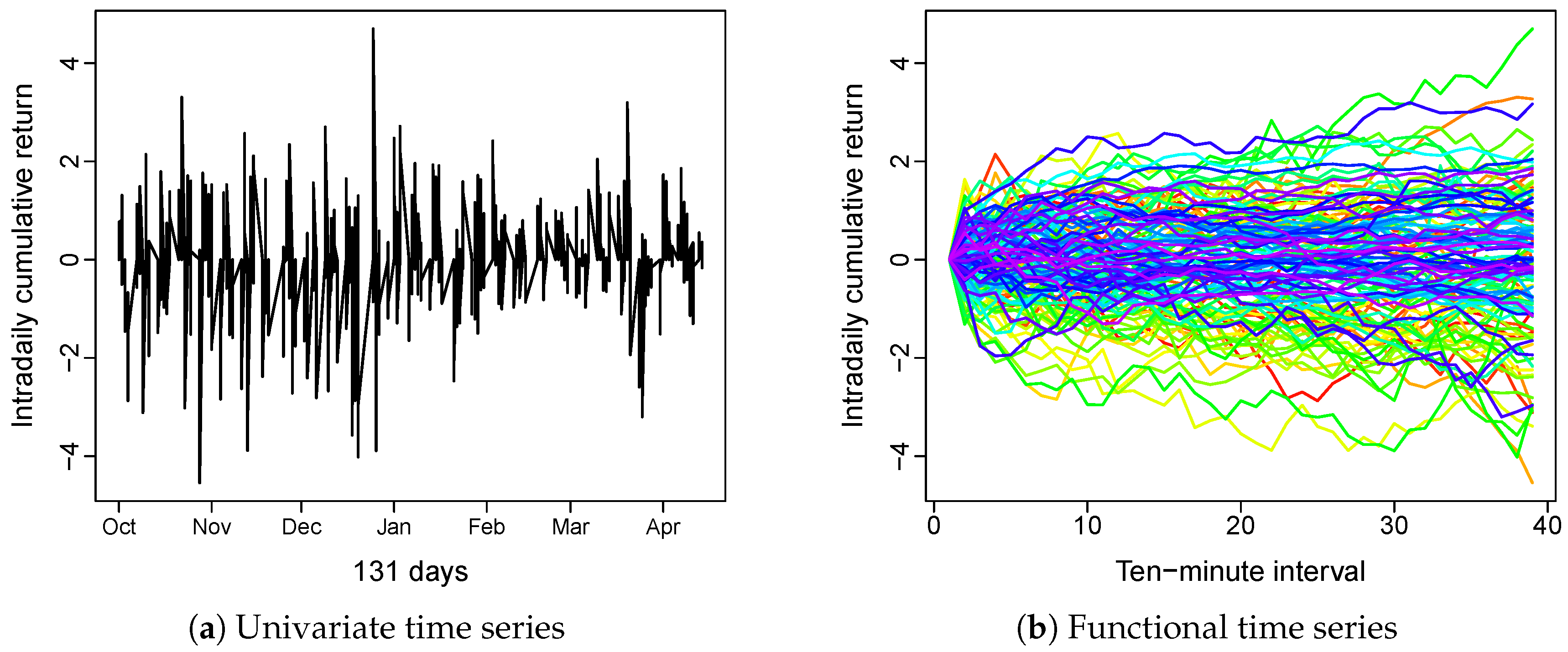
2.1. Data Conversion

Let $\{{\mathcal{Y}}_t\left(u\right):t=1,\dots ,T\}$ be the N-dimensional original FTS, where N is the number of sets of FTS, and T is the sample size or number of functions within each set of FTS. At each time t, ${\mathcal{Y}}_t\left(u\right)={[{\mathcal{Y}}_t^{\left(1\right)}\left(u\right),\dots ,{\mathcal{Y}}_t^{\left(N\right)}\left(u\right)]}^{\top }$, where each ${\mathcal{Y}}_t^{\left(i\right)}\left(u\right)$ is defined in $L^2\left(\mathcal{I}\right)$, a Hilbert space of square integrable functions on a real interval $\mathcal{I}\in [a,b]$, with the inner product $⟨f,g⟩={\int }_{\mathcal{I}}f\left(u\right)g\left(u\right)$ with the norm $\parallel ·\parallel ={⟨·,·⟩}^{\frac{1}{2}}$. If we focus on one dimension of the HDFTS, for each i, where $i=1,2,\dots ,N$, $\{{\mathcal{Y}}_t^{\left(i\right)}\left(u\right):t=1,\dots ,T\}$ represents the $i\mathrm{th}$ set of FTS.

In order to convert the HDFTS into matrix-valued time series, the measurement error is smoothed out so that the smoothness assumption is met, that is, observations at discretized grid points on the functions are sampled from the smoothed trajectories. Then, the values at discretized grid points of the HDFTS can be arranged into each matrix of the matrix-valued time series in the time sequence.

While there is no formal definition of “dense” functional data, conventional consent has been reached (Wang et al. 2016). Suppose each function, ${\mathcal{Y}}_t^{\left(i\right)}\left(u\right)$, is densely observed at discrete points $u_j$ for $j\in \{1,\dots ,J\}$ with errors such that

$${\mathcal{Y}}_t^{\left(i\right)}\left(u_j\right)={\mathcal{X}}_t^{\left(i\right)}\left(u_j\right)+{ϵ}_{t,j}^{\left(i\right)},$$

where ${\mathcal{X}}_t^{\left(i\right)}\left(u_j\right)$ is the smoothed trajectory observed at discrete point $u_j$, and ${ϵ}_{t,j}^{\left(i\right)}$ is the smooth error. Then, the discretized smooth HDFTS can be arranged into matrix-valued time series $\{{\mathit{X}}_t:t=1,\dots ,T\}$ such that

$${\mathit{X}}_t=\left[\begin{array}{cccc}{\mathcal{X}}_t^{\left(1\right)}\left(u_1\right)& {\mathcal{X}}_t^{\left(2\right)}\left(u_1\right)& \cdots & {\mathcal{X}}_t^{\left(N\right)}\left(u_1\right)\\ {\mathcal{X}}_t^{\left(1\right)}\left(u_2\right)& {\mathcal{X}}_t^{\left(2\right)}\left(u_2\right)& \cdots & {\mathcal{X}}_t^{\left(N\right)}\left(u_2\right)\\ ⋮& \ddots & \ddots & ⋮\\ {\mathcal{X}}_t^{\left(1\right)}\left(u_J\right)& {\mathcal{X}}_t^{\left(2\right)}\left(u_J\right)& \cdots & {\mathcal{X}}_t^{\left(N\right)}\left(u_J\right)\end{array}\right].$$

In the matrix-valued time series $\{{\mathit{X}}_t:t=1,\dots ,T\}$, the observation at time t, ${\mathit{X}}_t$, is a matrix where the $j\mathrm{th}$ column represents values at each grid point of the $t\mathrm{th}$ function of the $j\mathrm{th}$ set of smoothed FTS. Through the matrix conversion, we can preserve the different sets of information along the function (column-wise) and across the function (row-wise), and more importantly, we can capture the comovement of different grid points from different functions. Moreover, using the smoothed functional data instead of the original functional data with measurement error allows us to pool observations at neighboring grid points so that the benefits brought by the smoothness assumption of FDA can be employed.

2.2. Model

Applying the matrix factor model of Wang et al. (2019) to the matrix-valued time series converted from the HDFTS, we assume a few latent factors drive the HDFTS. Unlike the classical factor model, the factor is in a matrix form, and we use two loadings to capture the dependency across the row and the column. The matrix factor model for ${\mathit{X}}_t$ can be expressed as

$${\mathit{X}}_t={\lambda }^{\prime }{\mathit{F}}_t\mathsf{\Phi }+{ϵ}_t,t=1,\dots ,T,$$

(1)

where ${\mathit{F}}_t$ is an $r\times k$ unobserved matrix-valued time series of common fundamental factors, ${\lambda }^{\prime }$ is a $J\times r$ front loading matrix, $\mathsf{\Phi }$ is $k\times N$ back loading matrix, and ${ϵ}_t$ is an $J\times N$ error matrix.

2.3. Interpretation

The front loading matrix corresponds to the row effect, while the back loading matrix corresponds to the column effect. Equation (1) can be expressed in matrix format  

$$\begin{array}{c}\hfill \left[\begin{array}{ccc}{X}_t^{\left(1\right)}\left(u_1\right)& \cdots & X_t^{\left(N\right)}\left(u_1\right)\\ ⋮& \ddots & ⋮\\ X_t^{\left(1\right)}\left(u_J\right)& \cdots & X_t^{\left(N\right)}\left(u_J\right)\end{array}\right]=\left[\begin{array}{ccc}{\lambda }_{11}& \cdots & {\lambda }_{r1}\\ ⋮& \ddots & ⋮\\ {\lambda }_{1J}& \cdots & {\lambda }_{rJ}\end{array}\right]·\left[\begin{array}{ccc}{F}_{t,11}& \cdots & F_{t,1k}\\ ⋮& \ddots & ⋮\\ F_{t,r1}& \cdots & F_{t,rk}\end{array}\right]·\left[\begin{array}{ccc}{\mathsf{\Phi }}_{11}& \cdots & {\mathsf{\Phi }}_{1N}\\ ⋮& \ddots & ⋮\\ {\mathsf{\Phi }}_{k1}& \cdots & {\mathsf{\Phi }}_{kN}\end{array}\right]\end{array}$$

(2)

To view the effect of one loading matrix separately, we set the other front loading as an identity matrix. To isolate the column effect, assuming $\lambda$ is a $J\times J$ identity matrix, the model in (1) can be expressed as ${\mathit{X}}_t={\mathit{F}}_t\mathsf{\Phi }+{ϵ}_t$, where ${\mathit{F}}_t$ is a $J\times k$ matrix, and $\mathsf{\Phi }$ is the $k\times N$ loading matrix. Equation (2) can be expressed as

$$\begin{array}{c}\hfill \left[\begin{array}{ccc}{X}_t^{\left(1\right)}\left(u_1\right)& \cdots & X_t^{\left(N\right)}\left(u_1\right)\\ ⋮& \ddots & ⋮\\ X_t^{\left(1\right)}\left(u_J\right)& \cdots & X_t^{\left(N\right)}\left(u_J\right)\end{array}\right]=\left[\begin{array}{ccc}{F}_{t,11}& \cdots & F_{t,1k}\\ ⋮& \ddots & ⋮\\ F_{t,J1}& \cdots & F_{t,Jk}\end{array}\right]·\left[\begin{array}{ccc}{\mathsf{\Phi }}_{11}& \cdots & {\mathsf{\Phi }}_{1N}\\ ⋮& \ddots & ⋮\\ {\mathsf{\Phi }}_{k1}& \cdots & {\mathsf{\Phi }}_{kN}\end{array}\right]\\ \hfill =\left[\begin{array}{ccc}{F}_{t,11}·{\mathsf{\Phi }}_{11}+\dots +F_{t,1k}·{\mathsf{\Phi }}_{k1},& \cdots ,& F_{t,11}·{\mathsf{\Phi }}_{1N}+\dots +F_{t,1k}·{\mathsf{\Phi }}_{kN}\\ ⋮& \ddots & ⋮\\ F_{t,J1}·{\mathsf{\Phi }}_{11}+\dots +F_{t,Jk}·{\mathsf{\Phi }}_{k1},& \cdots ,& F_{t,J1}·{\mathsf{\Phi }}_{1N}+\dots +F_{t,Jk}·{\mathsf{\Phi }}_{kN}\end{array}\right]\end{array}$$

(3)

From (3), we can see that each column of ${\mathit{X}}_t$ is a linear combination of the columns of ${\mathit{F}}_t$. Taking the constituent stocks of an index as an example, where $\{{\mathcal{X}}_t^{\left(i\right)}\left(u\right):t=1,\dots ,T\}$ represents the intraday cumulative returns at given day t for specific stock i, at the trading time $u_1,\dots ,u_J$, J is the number of trading intervals. Then, the $i\mathrm{th}$ column of ${\mathit{X}}_t$ can be expressed as

$$\begin{array}{cc}\hfill {\mathrm{stock}}_i& {\mathit{f}}_{t,·1}{\mathit{f}}_{t,·k}\hfill \\ \hfill {\left[\begin{array}{c}{X}_t^{\left(i\right)}\left(u_1\right)\\ X_t^{\left(i\right)}\left(u_2\right)\\ ⋮\\ X_t^{\left(i\right)}\left(u_J\right)\end{array}\right]}_t& ={\mathsf{\Phi }}_{1i}\left[\begin{array}{c}{F}_{t,11}\\ F_{t,21}\\ ⋮\\ F_{t,J1}\end{array}\right]+\dots +{\mathsf{\Phi }}_{ki}\left[\begin{array}{c}{F}_{t,1k}\\ F_{t,2k}\\ ⋮\\ F_{t,Jk}\end{array}\right]+{ϵ}_{t,·i}.\hfill \end{array}$$

It can be seen that the intraday cumulative returns for trading time $u_j$ only depend on the $j\mathrm{th}$ row of ${\mathit{F}}_t$. Therefore, the $j\mathrm{th}$ row is the factor for trading time $u_j$. Since the front loading is $\mathit{I}$, there are no interactions among trading times. The back loading matrix $\mathsf{\Phi }$ reflects how each stock depends on columns of ${\mathit{F}}_t$ and hence captures column interactions, i.e., interactions among stocks.

Similarly, we assume $\mathsf{\Phi }$ is an $N\times N$ identity matrix to isolate the row effect. Then, (1) can be expressed as ${\mathit{X}}_t={\lambda }^{\prime }{\mathit{F}}_t+{ϵ}_t$, where ${\mathit{F}}_t$ is an $r\times N$ factor matrix, and $\lambda$ is an $r\times J$ loading matrix. Equation (2) can be expressed as

$$\begin{array}{c}\hfill \left[\begin{array}{ccc}{X}_t^{\left(1\right)}\left(u_1\right)& \cdots & X_t^{\left(N\right)}\left(u_1\right)\\ ⋮& \ddots & ⋮\\ X_t^{\left(1\right)}\left(u_J\right)& \cdots & X_t^{\left(N\right)}\left(u_J\right)\end{array}\right]=\left[\begin{array}{ccc}{\lambda }_{11}& \cdots & {\lambda }_{r1}\\ ⋮& \ddots & ⋮\\ {\lambda }_{1J}& \cdots & {\lambda }_{rJ}\end{array}\right]·\left[\begin{array}{ccc}{F}_{t,11}& \cdots & F_{t,1N}\\ ⋮& \ddots & ⋮\\ F_{t,r1}& \cdots & F_{t,rN}\end{array}\right]\\ \hfill =\left[\begin{array}{ccc}{\lambda }_{11}·F_{t,11}+\dots +{\lambda }_{r1}·F_{t,r1},& \dots & {\lambda }_{11}·F_{t,1N}+\dots +{\lambda }_{r1}·F_{t,rN}\\ ⋮& \ddots & ⋮\\ {\lambda }_{1J}·F_{t,11}+\dots +{\lambda }_{rJ}·F_{t,r1},& \dots & {\lambda }_{1J}·F_{t,1N}+\dots +{\lambda }_{rJ}·F_{t,rN}\end{array}\right]\end{array}$$

(4)

From (4), we can see that each row ${\mathit{X}}_t$ is a linear combination of the rows of ${\mathit{F}}_t$. The $j\mathrm{th}$ row of ${\mathit{X}}_t$, ${\mathit{X}}_t\left(u_j\right)=\{X_t^{\left(1\right)}\left(u_j\right),X_t^{\left(2\right)}\left(u_j\right),\dots ,X_t^{\left(N\right)}\left(u_j\right)\}$ can be expressed as

$$\begin{array}{cc}\hfill \left[\begin{array}{c}{X}_t^{\left(1\right)}\left(u_j\right),X_t^{\left(2\right)}\left(u_j\right),\dots ,X_t^{\left(N\right)}\left(u_j\right)\end{array}\right]& ={\lambda }_{1j}\left[\begin{array}{c}{F}_{t,11},F_{t,12},\dots ,F_{t,1N}\end{array}\right]{\mathit{f}}_{t,1·}\hfill \\ \hfill & +{\lambda }_{2j}\left[\begin{array}{c}{F}_{t,21},F_{t,22},\dots ,F_{t,2N}\end{array}\right]{\mathit{f}}_{t,2·}\hfill \\ \hfill & +\hfill \\ \hfill & ⋮\hfill \\ \hfill & +{\lambda }_{rj}\left[\begin{array}{c}{F}_{t,r1},F_{t,r2},\dots ,F_{t,rN}\end{array}\right]{\mathit{f}}_{t,r·}\hfill \\ \hfill & +{ϵ}_{t,j·}\hfill \end{array}$$

It can be seen that the intraday cumulative returns for stock i only depend on the $i\mathrm{th}$ column of ${\mathit{F}}_t$. Therefore, the $i\mathrm{th}$ column is the factor for stock i. The front loading matrix ${\lambda }^{\prime }$ reflects how trading time depends on rows of ${\mathit{F}}_t$ and hence captures row interactions, i.e., interactions among trading times.

Therefore, the matrix factor model could capture how the intraday cumulative returns for different stocks interact, and how the intraday cumulative returns at different trading times interact.

2.4. Estimation

We need to estimate $\lambda$, ${\mathit{F}}_t$, and $\mathsf{\Phi }$ in (1), respectively. Due to the latent nature of the factors, assumptions on the factors are made. Here, we follow the assumption that all dynamics of the observed processes are captured by the factors (Pan and Yao 2008; Lam et al. 2011; Lam and Yao 2012; Liu and Chen 2016; Wang et al. 2019). Moreover, for factor models, there exist identifiability issues among the factors, which means model (1) is not identifiable. However, similar to the argument of Lam et al. (2011), Lam and Yao (2012), Wang et al. (2019) argued that the column spaces of $\lambda$ and $\mathsf{\Phi }$ are uniquely determined. Hence, the problem will be converted to the estimation of the column spaces of $\lambda$ and $\mathsf{\Phi }$. We follow the idea in Lam et al. (2011), $\lambda$ and $\mathsf{\Phi }$ can be decomposed as

$$\lambda ={\mathit{W}}_{\mathbf{1}}{\mathit{Q}}_1,$$

and

$$\mathsf{\Phi }={\mathit{W}}_2{\mathit{Q}}_2$$

where ${\mathit{Q}}_1$ and ${\mathit{Q}}_2$ is $r\times J$ and $k\times N$ matrices, respectively, with orthonormal rows, ${\mathit{W}}_1$ and ${\mathit{W}}_2$ are $r\times r$ and $k\times k$ nonsingular matrices, respectively. Then $\lambda$ will have the same column space as ${\mathit{Q}}_1$ and $\mathsf{\Phi }$ will have the same column space ${\mathit{Q}}_2$. Let

$${\mathbf{Z}}_t={\mathit{W}}_1^{\prime }{\mathit{F}}_t{\mathit{W}}_2$$

Then (1) can be expressed as

$${\mathit{X}}_t={\mathit{Q}}_1^{\prime }{\mathbf{Z}}_t{\mathit{Q}}_2+{ϵ}_t$$

The estimation problem becomes estimating ${\mathit{Q}}_1$ and ${\mathit{Q}}_2$ (see Lam et al. 2011; Wang et al.2019, for details). Since ${\mathit{Q}}_1$ and ${\mathit{Q}}_2$ are orthonormal, so are their estimators, ${\hat{\mathit{Q}}}_1$ and ${\hat{\mathit{Q}}}_2$, therefore

$${\hat{\mathbf{Z}}}_t={\hat{\mathit{Q}}}_1{\mathit{X}}_t{\hat{\mathit{Q}}}_2^{\prime }$$

(5)

Then, ${\hat{\mathit{Q}}}_1^{\prime }$, ${\hat{\mathbf{Z}}}_t$ and ${\hat{\mathit{Q}}}_2$ will be the estimators of $\lambda$, ${\mathit{F}}_t$ and $\mathsf{\Phi }$, respectively.

3. Forecasting Method

In this section, we outline the matrix-valued factor model and the methods we used for comparison (Gao et al. 2019; Hyndman and Shang 2009). More specifically, we outline ways to generate point forecasts and interval forecasts for each method.

3.1. Point Forecasts

3.1.1. Matrix-Valued Factor Model

With the matrix-valued factor model, the information of the high-dimensional functional time series are contained and well preserved in the matrix-valued time series of the latent factors, ${\mathit{F}}_t$. Hence, we could make forecasts on the time series of estimated latent factors and then recover the original high-dimensional functional time series using (1) to generate the forecasts of the high-dimensional functional time series. Here, we apply the univariate time series forecasting method of Hyndman and Shang (2009) to make a forecast of the estimated latent factors. More specifically, we fit $r\times k$ ARMA models on the estimate factors $\left\{{\hat{F}}_{1,sq},\dots ,{\hat{F}}_{t,sq}\right\}$, where $s\in \{1,\dots ,r\}$ and $q\in \{1,\dots ,k\}$.

The h-step ahead forecast of the factor matrix ${\hat{\mathit{F}}}_{\kappa +h|\kappa }$ can be constructed as

$${\hat{\mathit{F}}}_{\kappa +h|\kappa }=\left[\begin{array}{ccc}{\hat{F}}_{\kappa +h|\kappa ,11}& \dots & {\hat{F}}_{\kappa +h|\kappa ,1k}\\ ⋮& \ddots & ⋮\\ {\hat{F}}_{\kappa +h|\kappa ,r1}& \dots & {\hat{F}}_{\kappa +h|\kappa ,rk}\end{array}\right]$$

where $\kappa$ is the number of observations used in the univariate time series for forecasting. With a set of holdout samples, the h-step-ahead point forecast for ${\mathit{X}}_t$ can be expressed as

$${\hat{\mathit{X}}}_{\kappa +h|\kappa }={\hat{\lambda }}^{\prime }{\hat{\mathit{F}}}_{\kappa +h|\kappa }\hat{\mathsf{\Phi }},$$

where $\hat{\lambda }$ and $\hat{\mathsf{\Phi }}$ are the estimates of $\lambda$ and $\mathsf{\Phi }$, respectively, and $\kappa$ is the number of observations used in generating the point forecasts.

3.1.2. Twofold Dimensional Reduction Model

In Gao et al. (2019), the dynamics across curves within each functional time series are captured by the long-run covariance kernel, which is defined as

$$C^{\left(i\right)}(u_r,u_s)=\sum _{q=-\infty }^{\infty }{\gamma }_q^{\left(i\right)}(u_r,u_s),\mathrm{where}{\gamma }_q^{\left(i\right)}(u_r,u_s)=\mathrm{cov}\left(X_0^{\left(i\right)}\left(u_r\right),X_q^{\left(i\right)}\left(u_s\right)\right)$$

The forecasting method of the twofold dimensional reduction model consists of three steps:

• Eigen analysis is performed on the estimated long-run covariance functions to reduce dimensions of functions into a finite number of principal components p(dynamic FPCA);
• The p principal components from N functional time series are organized into p vectors of length N. p Factor models is applied separately to these $N\times 1$ vectors of the principal component scores to further reduce the dimensions of the functional time series N into r so that we have $r\times p$ factors.
• Univariate time series model is fitted to each factor to produce forecasts of factors before constructing point forecasts of functions.

3.1.3. Univariate Functional Time Series Model

We incorporate the dynamic FPCA into the univariate functional time series model of Hyndman and Shang (2009) to capture the dynamics across curves within each functional time series. Different from Gao et al. (2019), a univariate time series model is applied to the principal components scores to produce forecasts directly instead of reducing the dimension of countries further. Then, the forecast principal components are used to construct a point forecast of functions.

From this point of view, we can see that in the second dimension reduction step, Gao et al. (2019) accommodate the problem of high dimension, which also captures the correlation among sets of functional time series, which is an extension of the univariate functional time series model of Hyndman and Shang (2009), while the correlation is reflected by the dimensional-reduced data, which has information loss. While the matrix factor model reduces the dimensions of both the functions and number of functional time series simultaneously, since the matrix structure is maintained, the information within the rows and the columns are well preserved.

3.2. Interval Forecasts

To capture the uncertainties in the point forecasts, we also construct the prediction intervals based on the point forecasts of each method. Aue et al. (2015) proposed a parametric approach for constructing uniform prediction intervals, which can be extended to pointwise prediction intervals after considering the nonparametric bootstrap approach of Shang (2018). For each stock i, based on the in-sample-forecast errors, ${\widehat{ϵ}}_{\kappa +h|\kappa }^{\left(i\right)}\left(u_j\right)=X_{\kappa +h}^{\left(i\right)}\left(u_j\right)-{\hat{X}}_{\kappa +h}^{\left(i\right)}\left(u_j\right)$, we use sampling with replacement to generate a series of bootstrapped forecast errors to obtain the upper bound and lower bound, ${\gamma }_{\mathrm{lb}}^{\left(i\right)}\left(u_j\right)$ and ${\gamma }_{\mathrm{ub}}^{\left(i\right)}\left(u_j\right)$, respectively. Then, a tuning parameter, ${\tau }_{\alpha }$, can be determined, such that

$$\mathbb{P}\left\{{\tau }_{\alpha }\times {\gamma }_{\mathrm{lb}}^{\left(i\right)}\left(u_j\right)\le {\widehat{ϵ}}_{\kappa +h|\kappa }^{\left(i\right)}\le {\tau }_{\alpha }\times {\gamma }_{\mathrm{ub}}^{\left(i\right)}\left(u_j\right)\right\}=(1-\alpha )\times 100\%.$$

Then, the h-step-ahead pointwise prediction interval for stock i is as follows:

$${\hat{X}}_{\kappa +h}^{\left(i\right)}\left(u_j\right)+{\tau }_{\alpha }\times {\gamma }_{\mathrm{lb}}^{\left(i\right)}\left(u_j\right)\le X_{\kappa +h}^{\left(i\right)}\left(u_j\right)\le {\hat{X}}_{\kappa +h}^{\left(i\right)}\left(u_j\right)+{\tau }_{\alpha }\times {\gamma }_{\mathrm{ub}}^{\left(i\right)}\left(u_j\right).$$

4. Measure Forecast Accuracy

This section outlines the measures of the accuracy of point forecasts and interval forecasts.

4.1. Point Forecast Accuracy Evaluation

We use the root mean square forecast error (RMSFE) of the h-step-ahead point forecasts to evaluate the point forecast accuracy. It measures how close the forecast results are to the actual values of the data being forecast.

The h-step-ahead point forecasts are generated using an expanding window analysis, which is commonly used in time series models to evaluate model stability. Using the expanding window analysis, we firstly use the first k observations to generate the h-step-ahead point forecasts for $h=1,2,\dots ,T-\kappa$. The forecast process is then iterated by increasing the sample size by one day until reaching the end period of the data. The RMSFE for the h-step-ahead forecasts of the $i\mathrm{th}$ stock can be written as

$${\mathrm{RMSFE}}_i\left(h\right)=\sqrt{\frac{1}{J\times (T-k-h+1)}\sum _{\kappa =k}^{T-h}\sum _{j=1}^J{\left[X_{\kappa +h}^{\left(i\right)}\left(u_j\right)-{\hat{X}}_{\kappa +h}^{\left(i\right)}\left(u_j\right)\right]}^2}$$

where $\kappa$ is the number of observations used in generating the point forecasts, then $X_{\kappa +h}^{\left(i\right)}\left(u_j\right)$ is the actual holdout sample for the $(\kappa +h)$ curve at trading time $u_j$ for stock i, and ${\hat{X}}_{\kappa +h}^{\left(i\right)}\left(u_j\right)$ is the h-step-ahead point forecasts for the holdout sample based on the first $\kappa$ curves, and J is the number of grid points of each curve.

4.2. Interval Forecast Accuracy Evaluation

We use the interval scoring rule of Gneiting and Raftery (2007) to evaluate the pointwise interval forecast accuracy. The interval score for the pointwise interval forecast at time point $x_i$ is

$$\begin{array}{cc}\hfill S_{\alpha }\left[{\hat{X}}_{\kappa +h}^{\left(i\right)\left(\mathrm{lb}\right)}\left(u_j\right),{\hat{X}}_{\kappa +h}^{\left(i\right)\left(\mathrm{ub}\right)}\left(u_j\right);X_{\kappa +h}^{\left(i\right)}\left(u_j\right)\right]& =\left[{\hat{X}}_{\kappa +h}^{\left(i\right)\left(\mathrm{ub}\right)}\left(u_j\right)-{\hat{X}}_{\kappa +h}^{\left(i\right)\left(\mathrm{lb}\right)}\left(u_j\right)\right]\hfill \\ \hfill & +\frac{2}{\alpha }\left[{\hat{X}}_{\kappa +h}^{\left(i\right)\left(\mathrm{lb}\right)}\left(u_j\right)-X_{\kappa +h}^{\left(i\right)}\left(u_j\right)\right]\mathbb{1}\left\{X_{\kappa +h}^{\left(i\right)}\left(u_j\right)<{\hat{X}}_{\kappa +h}^{\left(i\right)\left(\mathrm{lb}\right)}\left(u_j\right)\right\}\hfill \\ \hfill & +\frac{2}{\alpha }\left[X_{\kappa +h}^{\left(i\right)}\left(u_j\right)-{\hat{X}}_{\kappa +h}^{\left(i\right)\left(\mathrm{ub}\right)}\left(u_j\right)\right]\mathbb{1}\left\{X_{\kappa +h}^{\left(i\right)}\left(u_j\right)>{\hat{X}}_{\kappa +h}^{\left(i\right)\left(\mathrm{ub}\right)}\left(u_j\right)\right\}\hfill \end{array}$$

where the level of significance $\alpha$ can be chosen conventionally as $0.2$. It is not difficult to find that the smaller the interval score is, the more accurate the interval forecast. An optimal (which is also minimal) interval score value can be achieved if $X_{\kappa +h}^{\left(i\right)}\left(u_j\right)$ lies between ${\hat{X}}_{\kappa +h}^{\left(i\right)\left(\mathrm{lb}\right)}\left(u_j\right)$ and ${\hat{X}}_{\kappa +h}^{\left(i\right)\left(\mathrm{ub}\right)}\left(u_j\right)$. Then, the mean interval score for the h-step-ahead forecast of the $i\mathrm{th}$ stock can be written as

$${\overline{S}}_{\alpha }^{\left(i\right)}\left(h\right)=\frac{1}{J\times (T-k-h+1)}\sum _{\kappa =k}^{T-h}\sum _{j=1}^J{S}_{\alpha }\left[{\hat{X}}_{\kappa +h}^{\left(i\right)\mathrm{lb}}\left(u_j\right),{\hat{X}}_{\kappa +h}^{\left(i\right)\mathrm{ub}}\left(u_j\right);X_{\kappa +h}^{\left(i\right)}\left(u_j\right)\right]$$

5. Empirical Results

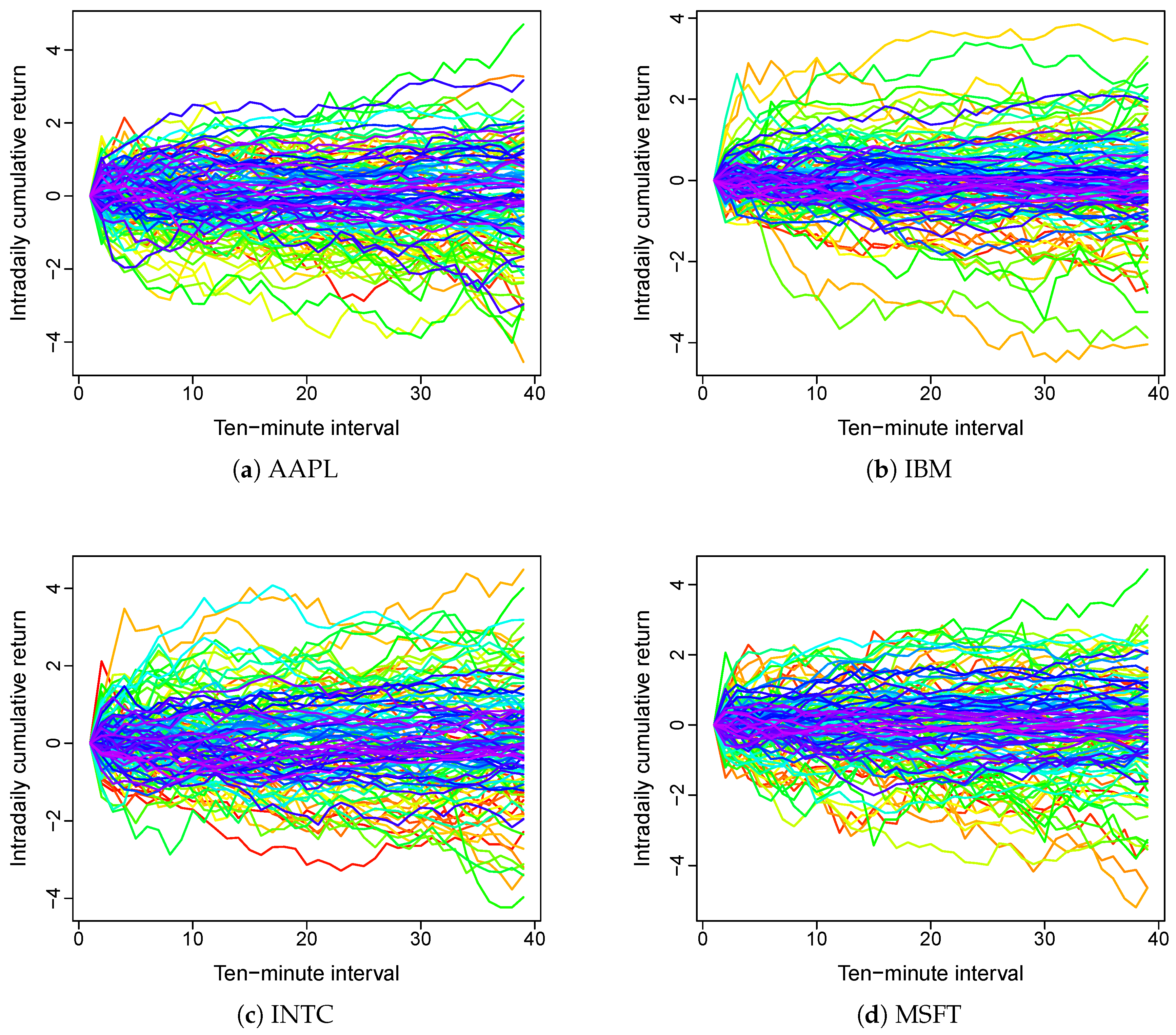
In this section, we employ the models described in Section 3 to model and forecast the DJIA constituent stocks.

5.1. Data

Originally published on 26 May 1896 and named after Charles Dow and Edward Jones, DJIA is the second-oldest US market index. It is often used as an indicator of the industrial sector in the US economy. The performance of DJIA can be influenced by many factors, such as corporate and economic reports, global political events, and all other incidents that may affect the economy. All financial crises in US history can be firstly reflected as the crashes of DJIA. Moreover, stock markets around the world are closely related to the performance of DJIA. Hence, producing accurate forecasts is of particularly important interest to all stakeholders and investors involved in activities related to DJIA. Those related parties may include governments, regulatory authorities, hedge and pension fund managers, and retailer investors.

We consider the intraday 10-min prices of 29 constituent stocks in DJIA from 3 October 2018 to 16 April 2019,1 which are sourced from Bloomberg. Table 1 list the names of these stocks and the corresponding symbols.

Table 1. List of constituent stocks in DJIA and corresponded symbols.

Company Name	Symbol
Apple Inc.	AAPL
American Express	AXP
The Boeing Company	BA
Caterpillar Inc.	CAT
Cisco Systems, Inc.	CSCO
Chevron Corporation	CVX
The Walt Disney Company	DIS
The Goldman Sachs Group, Inc.	GS
The Home Depot, Inc.	HD
International Business Machines Corporation	IBM
Intel Corporation	INTC
Johnson & Johnson	JNJ
JPMorgan Chase & Co.	JPM
The Coca-Cola Company	KO
McDonald’s Corporation	MCD
3M Company	MMM
Merck & Co., Inc.	MRK
Microsoft Corporation	MSFT
NIKE, Inc.	NKE
Pfizer Inc.	PFE
The Procter & Gamble Company	PG
The Travelers Companies, Inc.	TRV
UnitedHealth Group Incorporated	UNH
United Technologies Corporation	UTX
Visa Inc.	V
Verizon Communications Inc.	VZ
Walgreens Boots Alliance, Inc.	WBA
Walmart Inc.	WMT
Exxon Mobil Corporation	XOM

Due to the nonstationarity of the intraday price curves, we calculate returns based on those curves to drive stationary curves (Gabrys et al. 2010; Kokoszka et al. 2015) as

$$r_n\left(u_j\right)=100\times [\ln P_n\left(u_j\right)-\ln P_n\left(u_1\right)]$$

where $P_n\left(u_j\right)$ is the price of a share at time $u_j$, for $j\in \{1,\dots ,J\}$, and J is the number of grid points at which price are observed. Essentially, we assume that the intraday cumulative returns are observed at discrete time points $u_j$ from a continuous intraday cumulative return curve ${\mathcal{X}}_t$. As for the DJIA data, J is 39, representing 39 ten-minute trading intervals over the six and half hours of each trading day.

Functional time series consists of a set of random functions observed at regular time intervals, with two broad categories. One is a segmentation of an almost continuous time record into natural consecutive intervals, such as days, months, or quarters, where the continuum of each function is a time variable (see, for example, Hörmann and Kokoszka 2012). The other type arises when each of the observations in a time period represents a continuous function, where the continuum is a variable other than time (see, for example, Chiou and Müller 2009). The intraday cumulative return curves are examples of the first category. More specifically, the intraday data are segments of longer time series, and a collection of such daily curves forms the functional time series.

Figure 1 displays the intraday cumulative returns of Apple Inc. In Figure 1a, we plot the intraday cumulative returns as a univariate time series, and in Figure 1b, we segment the univariate time series into daily curves. The collection of daily curves then form functional time series. We utilize the rainbow plot of Hyndman and Shang (2010) to show the time ordering of functional time series, where the curves from older times are in red, and the more recent curves are in purple.

Figure 1. Univariate and functional time series of intraday cumulative returns of AAPL. The univariate time series is the intraday cumulative return of APPL over 131 days, and the functional time series is the intraday cumulative return of APPL based on data of these 131 days, sliced into 10-min intervals. In the rainbow plot, the curves from older times are in red and the more recent curves are in purple.

Figure 2 displays the functional time series of intraday cumulative of four selected tech companies. Apparently, shapes of those functional time series are similar to each other. This suggests that the intraday cumulative returns of these shares are correlated. Hence, it is important to consider both the dynamics within each functional time series and their pairwise correlations.

Figure 2. Functional time series of intraday cumulative returns of four selected tech companies. It is the differences in the color patterns and shapes of curves that make functional time series different.

5.2. Forecast Evaluation

We used three different methods to generate five-step-ahead point and interval forecasts, that is, we only forecast the cumulative intraday return up to 5 days. Table 2 presents the averaged RMSFE values and averaged interval scores across all stocks in the holdout sample for the different forecast methods. The bold entries highlight the method that produces the best forecasts.

Table 2. Average RMSFE and interval scores.

	Averaged RMSFE			Averaged Interval Score
h	UFTS	HDFTS	MFMTS	UFTS	HDFTS	MFMTS
1	0.7570	0.7502	0.7312	2.5381	2.5489	2.5296
2	0.7535	0.7483	0.7283	2.8369	2.8199	2.7830
3	0.7541	0.7452	0.7305	3.1635	3.1614	3.1495
4	0.7702	0.7581	0.7421	3.2891	3.2150	3.2054
5	0.7579	0.7500	0.7330	2.3043	2.3278	2.2883

Notes: Average RMSFE values and averaged interval scores in the holdout sample based on different forecasting methods are presented in this table. Bold numbers indicate the smallest error for each dataset. Forecasts based on univariate functional time series are labeled as “UFTS”, forecasts based on twofold dimensional reduction model are labeled as “HDFTS”, and forecasts based on the matrix factor model are labeled as “MFMTS”.

It is obvious that our method produces the smallest averaged RMSFE values, the twofold dimensional reduction model performs the second, and the univariate functional time series model performs the worst. Further, the pairwise Diebold–Mariano tests are conducted on the RMSFE values, and significant test results are obtained at a 5% level in all cases. This suggests that the improvements of our model over the competitors are statistically significant. This is because that the univariate functional time series model ignores the correlation of functional time series, and the twofold dimensional reduction model is based on the dimension reduced data, which may not fully reflect all the information in the correlations among stocks.

In terms of the interval forecast, the same results can be observed, i.e., our method produces the smallest mean interval score values, which means that our method performs the best in producing interval forecasts.

After comparing all the point and interval forecast results for different methods, our proposed method outperforms other competitive methods. This means that forecasts based on our model provide a more robust forecast with less variation.

6. Conclusions

By applying the factor model matrix-valued to functional data, a forecasting method for high-dimensional functional time series is proposed. The matrix factor model could reduce the dimensions of functions and number of functional time series simultaneously; this is beneficial as it maintains the matrix structure of the original data, which could result in more efficient dimensional reduction as the information carried by rows and columns are well preserved. Ultimately, this will improve forecasting accuracy.

The study on constituent stocks in the Dow Jones Industrial Average (DJIA) illustrates the merits of our model as it produces more accurate and robust forecasts than the high-dimensional functional time series method by Gao et al. (2019) and the univariate functional time series method by Hyndman and Shang (2009).

In summary, our proposed matrix factor model could be a useful tool for modeling high-dimensional correlated financial time series where the number of financial time series are relatively large, compared to the sample size T. It is worth noting that the novel COVID-19 pandemic has caused large volatilities in all financial markets. This may suggest structural changes in the parametric structure, which is beyond the scope of this paper. Future extensions may be therefore conducted to investigate the incorporating of structural changes, as well as the robust methodologies to address the potential outliers.

References

- Aue, Alexander, Diogo Dubart Norinho, and Siegfried Hörmann. 2015. On the prediction of stationary functional time series. Journal of the American Statistical Association 110: 378–92. [Google Scholar] [CrossRef] [Green Version]
- Berrendero, José Ramón, Ana Justel, and Marcela Svarc. 2011. Principal components for multivariate functional data. Computational Statistics & Data Analysis 55: 2619–34. [Google Scholar]
- Bühlmann, Peter, and Sara Van De Geer. 2011. Statistics for High-Dimensional Data: Methods, Theory and Applications. Berlin: Springer Science & Business Media. [Google Scholar]
- Cai, Tony, and Xiaotong Chen. 2010. High-Dimensional Data Analysis. Beijing: Higher Education Press. [Google Scholar]
- Cardot, Hervé. 2000. Nonparametric estimation of smoothed principal components analysis of sampled noisy functions. Journal of Nonparametric Statistics 12: 503–38. [Google Scholar] [CrossRef]
- Chiou, Jeng-Min, Yu-Ting Chen, and Ya-Fang Yang. 2014. Multivariate functional principal component analysis: A normalization approach. Statistica Sinica 24: 1571–96. [Google Scholar] [CrossRef] [Green Version]
- Chiou, Jeng-Min, and Hans-Georg Müller. 2009. Modeling hazard rates as functional data for the analysis of cohort lifetables and mortality forecasting. Journal of the American Statistical Association 104: 572–85. [Google Scholar] [CrossRef] [Green Version]
- Ferraty, Frédéric, and Philippe Vieu. 2006. Nonparametric Functional Data Analysis: Theory and Practice. Berlin: Springer Science & Business Media. [Google Scholar]
- Gabrys, Robertas, Lajos Horváth, and Piotr Kokoszka. 2010. Tests for error correlation in the functional linear model. Journal of the American Statistical Association 105: 1113–25. [Google Scholar] [CrossRef]
- Gao, Yuan, Han Lin Shang, and Yanrong Yang. 2019. High-dimensional functional time series forecasting: An application to age-specific mortality rates. Journal of Multivariate Analysis 170: 232–43. [Google Scholar] [CrossRef] [Green Version]
- Gneiting, Tilmann, and Adrian E. Raftery. 2007. Strictly proper scoring rules, prediction, and estimation. Journal of the American Statistical Association 102: 359–78. [Google Scholar] [CrossRef]
- Hays, Spencer, Haipeng Shen, and Jianhua Z. Huang. 2012. Functional dynamic factor models with application to yield curve forecasting. The Annals of Applied Statistics 6: 870–94. [Google Scholar] [CrossRef]
- Hörmann, Siegfried, ukasz Kidziński, and Marc Hallin. 2015. Dynamic functional principal components. Journal of the Royal Statistical Society: Series B (Statistical Methodology) 77: 319–48. [Google Scholar] [CrossRef]
- Hörmann, Siegfried, and Piotr Kokoszka. 2012. Functional time series. In Handbook of Statistics. Edited by Tata Subba Rao, Suhasini Subba Rao and Calyampudi Radhakrishna Rao. Amsterdam: Elsevier, vol. 30, pp. 157–86. [Google Scholar]
- Horváth, Lajos, and Piotr Kokoszka. 2012. Inference For Functional Data with Applications. New York: Springer Science & Business Media. [Google Scholar]
- Hyndman, Rob J., and Han Lin Shang. 2009. Forecasting functional time series. Journal of the Korean Statistical Society 38: 199–211. [Google Scholar] [CrossRef]
- Hyndman, Rob J., and Han Lin Shang. 2010. Rainbow plots, bagplots, and boxplots for functional data. Journal of Computational and Graphical Statistics 19: 29–45. [Google Scholar] [CrossRef] [Green Version]
- Jungbacker, Borus, Siem Jan Koopman, and Michel Van Der Wel. 2014. Smooth dynamic factor analysis with application to the US term structure of interest rates. Journal of Applied Econometrics 29: 65–90. [Google Scholar] [CrossRef]
- Kokoszka, Piotr, Hong Miao, and Xi Zhang. 2015. Functional dynamic factor model for intraday price curves. Journal of Financial Econometrics 13: 456–77. [Google Scholar] [CrossRef] [Green Version]
- Kokoszka, Piotr, and Matthew Reimherr. 2017. Introduction to Functional Data Analysis. Cleveland: CRC press. [Google Scholar]
- Lam, Clifford, and Qiwei Yao. 2012. Factor modeling for high-dimensional time series: Inference for the number of factors. The Annals of Statistics 40: 694–726. [Google Scholar] [CrossRef] [Green Version]
- Lam, Clifford, Qiwei Yao, and Neil Bathia. 2011. Estimation of latent factors for high-dimensional time series. Biometrika 98: 901–18. [Google Scholar] [CrossRef]
- Liebl, Dominik. 2013. Modeling and forecasting electricity spot prices: A functional data perspective. The Annals of Applied Statistics 7: 1562–92. [Google Scholar] [CrossRef] [Green Version]
- Liu, Xialu, and Rong Chen. 2016. Regime-switching factor models for high-dimensional time series. Statistica Sinica 26: 1427–51. [Google Scholar] [CrossRef]
- Martínez-Hernández, Israel, Jesús Gonzalo, and Graciela González-Farías. 2020. Nonparametric estimation of functional dynamic factor model. arXiv arXiv:2011.01831. [Google Scholar]
- Pan, Jiazhu, and Qiwei Yao. 2008. Modelling multiple time series via common factors. Biometrika 95: 365–79. [Google Scholar] [CrossRef] [Green Version]
- Panaretos, Victor M., and Shahin Tavakoli. 2013. Cramér–karhunen–loève representation and harmonic principal component analysis of functional time series. Stochastic Processes and their Applications 123: 2779–807. [Google Scholar] [CrossRef]
- Ramsay, James O., and Bernard W. Silverman. 2006. Functional Data Analysis. New York: Springer Science & Business Media. [Google Scholar]
- Rice, Gregory, and Han Lin Shang. 2017. A plug-in bandwidth selection procedure for long-run covariance estimation with stationary functional time series. Journal of Time Series Analysis 38: 591–609. [Google Scholar] [CrossRef] [Green Version]
- Shang, Han Lin. 2017. Forecasting intraday s&p 500 index returns: A functional time series approach. Journal of Forecasting 36: 741–55. [Google Scholar]
- Shang, Han Lin. 2018. Bootstrap methods for stationary functional time series. Statistics and Computing 28: 1–10. [Google Scholar] [CrossRef] [Green Version]
- Shang, Han Lin, Yang Yang, and Fearghal Kearney. 2019. Intraday forecasts of a volatility index: Functional time series methods with dynamic updating. Annals of Operations Research 282: 331–54. [Google Scholar] [CrossRef] [Green Version]
- Wang, Dong, Xialu Liu, and Rong Chen. 2019. Factor models for matrix-valued high-dimensional time series. Journal of Econometrics 208: 231–48. [Google Scholar] [CrossRef] [Green Version]
- Wang, Jane-Ling, Jeng-Min Chiou, and Hans-Georg Müller. 2016. Functional data analysis. Annual Review of Statistics and Its Application 3: 257–95. [Google Scholar] [CrossRef] [Green Version]
- Zhang, Jin-Ting, and Jianwei Chen. 2007. Statistical inferences for functional data. The Annals of Statistics 35: 1052–79. [Google Scholar] [CrossRef] [Green Version]
- Zhang, Xiaoke, and Jane-Ling Wang. 2016. From sparse to dense functional data and beyond. The Annals of Statistics 44: 2281–321. [Google Scholar] [CrossRef]
Publisher’s Note: MDPI stays neutral with regard to jurisdictional claims in published maps and institutional affiliations. |
© 2021 by the authors. Licensee MDPI, Basel, Switzerland. This article is an open access article distributed under the terms and conditions of the Creative Commons Attribution (CC BY) license (https://creativecommons.org/licenses/by/4.0/).