First to React Is the Last to Forgive: Evidence from the Stock Market Impact of COVID 19

Abstract

The COVID 19 pandemic has had wide-ranging and severe effects on global economies. Stock markets as usual were the first to react, with drop rates as much as the global financial crises of 2008. This study uses daily data to model the dynamic impact of the COVID 19 pandemic on the first affected countries’ stock market indices and the global commodity markets. The panel least squares Vector Auto-Regressive (VAR) estimation results confirm the negative short-termed impact of the virus spread rate on the returns of the stock market indices. The spread rate is also significant to explain changes related to the prices of platinum, silver, West Texas Intermediate (WTI), and Brent crude oil.

1. Background

As the world is getting ready for a new year, health authorities in Wuhan, China has reported to the World Health Organization (WHO) the outbreak of an unknown cluster of viral pneumonia cases on the last day of December 2019. After a formal investigation of these cases by the beginning of 2020, the world witnessed the birth of the SARS‑CoV‑2 (COVID 19) virus. As of 15 December, more than 73 million infection cases and more than 1,600,000 deaths have been globally declared to be associated with COVID 19 pandemic (World Health Organization (WHO 2020). COVID 19 is the fifth in the 21st-century list of pandemics, after Influenza H1N1, Coronavirus (Bats), and Ebolavirus, Coronavirus (Camels). H1N1 is the furriest among the list as it was associated with 151,700 to 575,400 deaths worldwide (Center for Disease Control and Prevention (CDC 2019).

While the exact global economic impacts of COVID 19 are not yet clear, it is considered deadlier than the other two Coronaviruses and has affected a massively larger number of people over a shorter period. SARS and MERS have affected respectively, 8437 and 2499 cases, and with 813 and 816 associated deaths (WHO 2012; CDC 2004). This study contributes to the newly developed COVID 19 empirical research by examining the impact of the COVID 19 contamination rate on returns of stock market indices and prices of selected globally trade commodities, namely gold, platinum, silver, WTI, and Brent oil. We utilize daily data of selected stock markets from the firstly affected countries, China, the USA, Spain, Italy, South Korea, and Japan. The methodology adopted is a k-variate panel VAR of order $\mathrm{p}$ based on (Abrigo and Love 2016).

The overall panel least squares VAR estimation indicates a negative short termed impact of 2.3% in the performances of the stock markets when the spread rate of coronavirus increases by 1% across countries in time ceteris paribu. The coronavirus contamination rate is not statistically significant to explain the changes in the exchange rate and the growth of the prices of gold in the countries of analysis, regardless of this result, the virus spread rate is significant at the 90% confidence level to explain changes related to the prices of platinum, silver, WTI, and Brent crude oil. According to the Driscoll–Kraay approach, we found that the fluctuations of the exchange rate, platinum, and gold prices are the main drivers for stock market movements.

Global stock markets reacted strongly and wildly to the outbreak of COVID 19. In March 2020, the US stock market hit the circuit breaker mechanism four times in ten days. Since its inception in 1987, the breaker has only ever been triggered once, in 1997. Stock markets in Europe and Asia have also dramatically reacted. FTSE of the UK has dropped on the 12th of March more than 10% on its worst day since 1987 and the stock market in Japan has lost more than 20% from its highest position at the end of 2019 (Zhang et al. 2020). Gormsen and Koijen (2020) showed that stock markets have dropped in response to COVID 19 as much as the global financial crises of 2008, yet the markets during the pandemic have recovered quicker especially in Europe.

The pandemic severity varies across countries hence begetting non-uniform individual stock markets reactions, Capelle-Blancard and Desroziers (2020) have accounted for such heterogeneity across 74 countries and found that the number of infected people in each country was the primary driver for stock market reactions, and volatility heaved as concerns about the pandemic grew. Their results also showed that the number of COVID 19 infection cases in wealthy neighboring countries has affected investors’ decisions. He et al. (2020) used conventional t-tests and non-parametric Mann–Whitney tests to analyze the impact of COVID 19 on selected stock markets in Asia and Europe. They found that COVID 19 has a negative, bidirectional, and short-termed impact on stock markets between Asian, American, and European stock markets, yet the impact tends to intensify as the virus spreads.

Examining a different perspective of heterogeneity, Albuquerque et al. (2020) argued that COVID 19 have triggered unparalleled shocks to stocks, those with higher Environmental, Social, and Governance activities (ESG) rating have shown more resilience, maintained higher returns and higher operating profit margins relative to their counterparts during the first quarter of 2020. The logic here follows Albuquerque et al. (2019) model that investing in ESG policies feeds into the firms’ customer loyalty and reduces the price elasticity of demand for their products.

2. Literature Review

Studies of the macroeconomic impact of past pandemics have mainly aimed to quantify the effects in terms of lost output and growth, however firm conclusions about the pandemics’ long-run economic effects have not been well researched (Bell and Lewis 2004). Studies of such a scope usually study the short-term economic effects of pandemics through their impact on supply and demand, stock market, fertility rate, trade, labor inputs, and tourism (Jonung and Roeger 2006).

One of the few studies on the economic effects of Spanish influenza between 1918–1919, suggested that this pandemic has stimulated the growth of the US economy post the pandemic years in the 1920s (Brainerd and Siegler 2003), contrary to Correia et al. (2020) who showed that a sharp decline in economic activity has persisted until at least 1923. Comparing the Spanish flu effects across 43 countries between 1918 and 1920, Barro et al. (2020) concluded that the flu-associated death rates caused declines in GDP and consumption of about 6%. Karlsson et al. (2014) found no discernible effect of the 1918 influenza pandemic on earnings in Sweden. The state of the economy during a pandemic defines extensively the speed and severity of the ensued economic effects. Benmelech and Frydman (2020) argued that the increase in the government’s demand for World War I-related products during the 1918 influenza pandemic has made up for the contraction in consumer spending and private investment, leaving only modest and short-termed effects on US and European economies. It is generally perceived also that during pandemics, regions with a higher degree of global exposure and economic integration are affected more sturdily than less integrated regions (Verikios et al. 2012).

May 2009 witnessed the emergence of a new H1N1 commonly known as “swine flu” due to its close association with North American and Eurasian pig influenza. Verikios et al. (2012) is one of the few studies that investigated the economic effects of the H1N1 epidemic, by applying on Australia, their MONASH. Health model simulation results showed that the epidemic is associated with significant short-termed adverse macroeconomic effects that extend only within two or four quarters then the economy reverts to normal rates. The preceded contractionary effect would reduce tourism, household demands for international travel and industries would face increased costs via absenteeism and loss of labor force (Verikios et al. 2012).

As we move forward in time and from north to south on the map, Young (2005) projected an increasing trend in per capita consumption post the AIDS epidemic in South Africa. The widespread community infection measures during the epidemic have lowered national fertility rates, both directly, through a reduction in the willingness to engage in unprotected sexual activity and increasing the scarcity of labor and the value of a woman’s time. On contrary, the World Bank (2016) postulated that the recent Ebola epidemic in West Africa during 2014–2015 has had severe and adverse shocks to the private sector as well as has posed threats to national food security due to the decline in agricultural production.

Regarding the impact of the current COVID 19 pandemic on the global financial markets, Baker et al. (2020) stated that the US stock market has reacted more forcefully to the current pandemic than any other pandemic in the US history. Albulesco (2020) showed that the news about the new infection cases has enhanced the volatility of the United States S&P 500. Similar findings were portrayed by Zhang et al. (2020) on a global sample. Ashraf (2020b) studied the impact of COVID 19 on stock market returns using a global sample of 64 countries and found that stock market returns declined as the number of confirmed cases increased. Bakas and Triantafyllou (2020) analyzed the impact of the pandemic on global commodity markets, they showed that the pandemic uncertainty has decreased the volatility of commodity markets, especially on the crude oil market, while the effect on the gold market is positive but less significant.

Following a similar approach to our paper, but by applying to Africa, Takyi and Bentum-Ennin (2020) estimated the negative impact of COVID 19 on stock market performance to between 2.7% and 21% across their sample of 13 countries. Markets react un-uniformly to COVID 19 shocks, one possible reason according to Ashraf (2020a) is the level of cultural uncertainty avoidance, meaning that investors in countries with a higher level of uncertainty aversion are more likely to engage in panic selling to avoid uncertainty causing this market to be more vulnerable to COVID 19 shock relative to their counterparts. Engelhardt et al. (2020) suggest that high- trust levels between fellow citizens as well as for the government, contribute largely to reducing market volatility in response to the COVID 19 announcements. This paper contributes to the growing literature on the stock market effects of the COVID 19 pandemic. Using a sample of the 6 first affected countries, we use panel K VAR methodology to capture the interdependencies and homogeneity between COVID 19 contamination rate, stock market return, and selected global market commodities across countries and time.

3. Stylized Facts

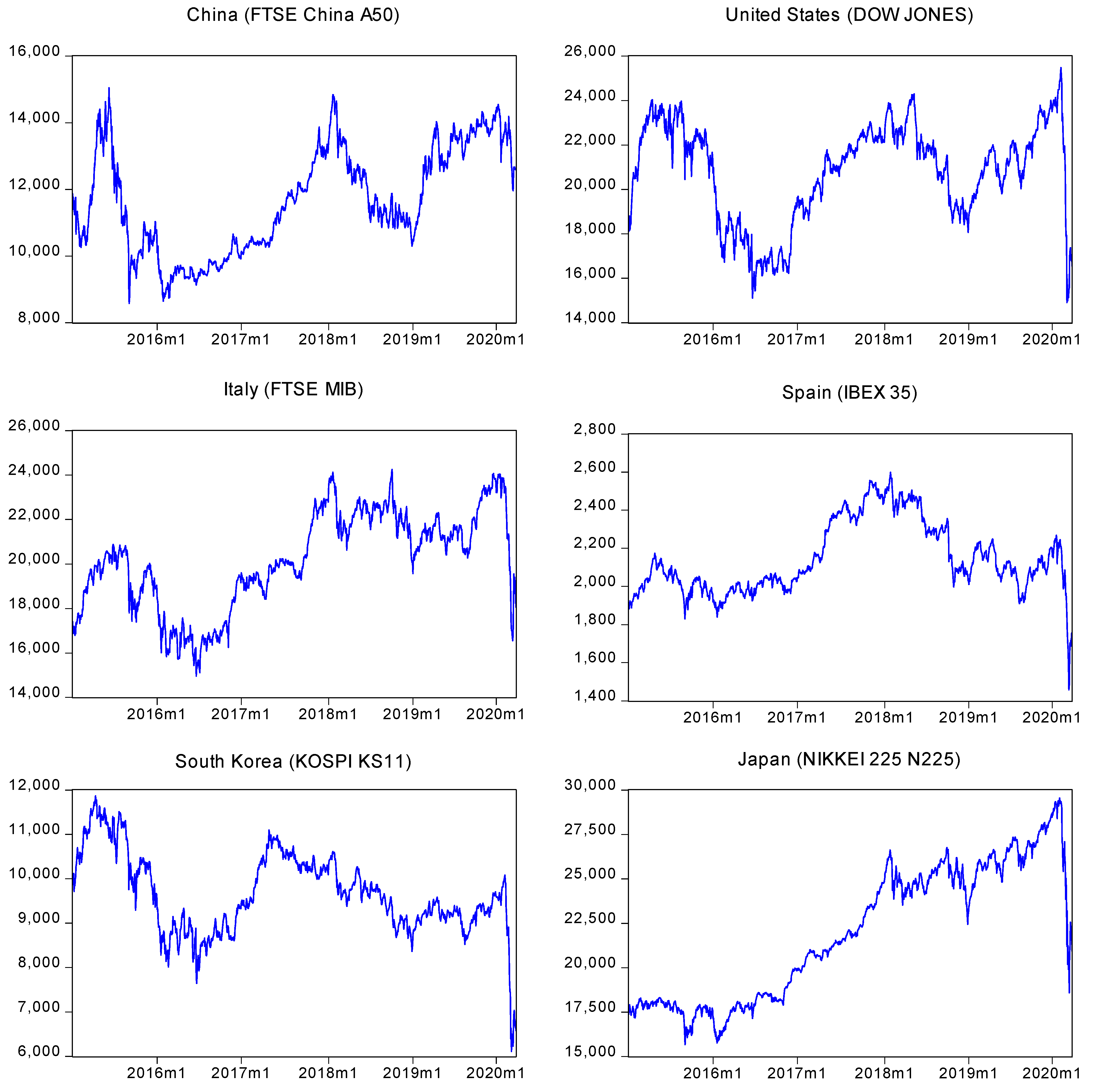
Since the outbreak of the COVID 19 in January 2020 and on, a persistent decrease in stock market returns is observed in Figure 1 in the first affected countries.

Figure 1. Stock market prices in local currencies. Source: Data Stream (2020).

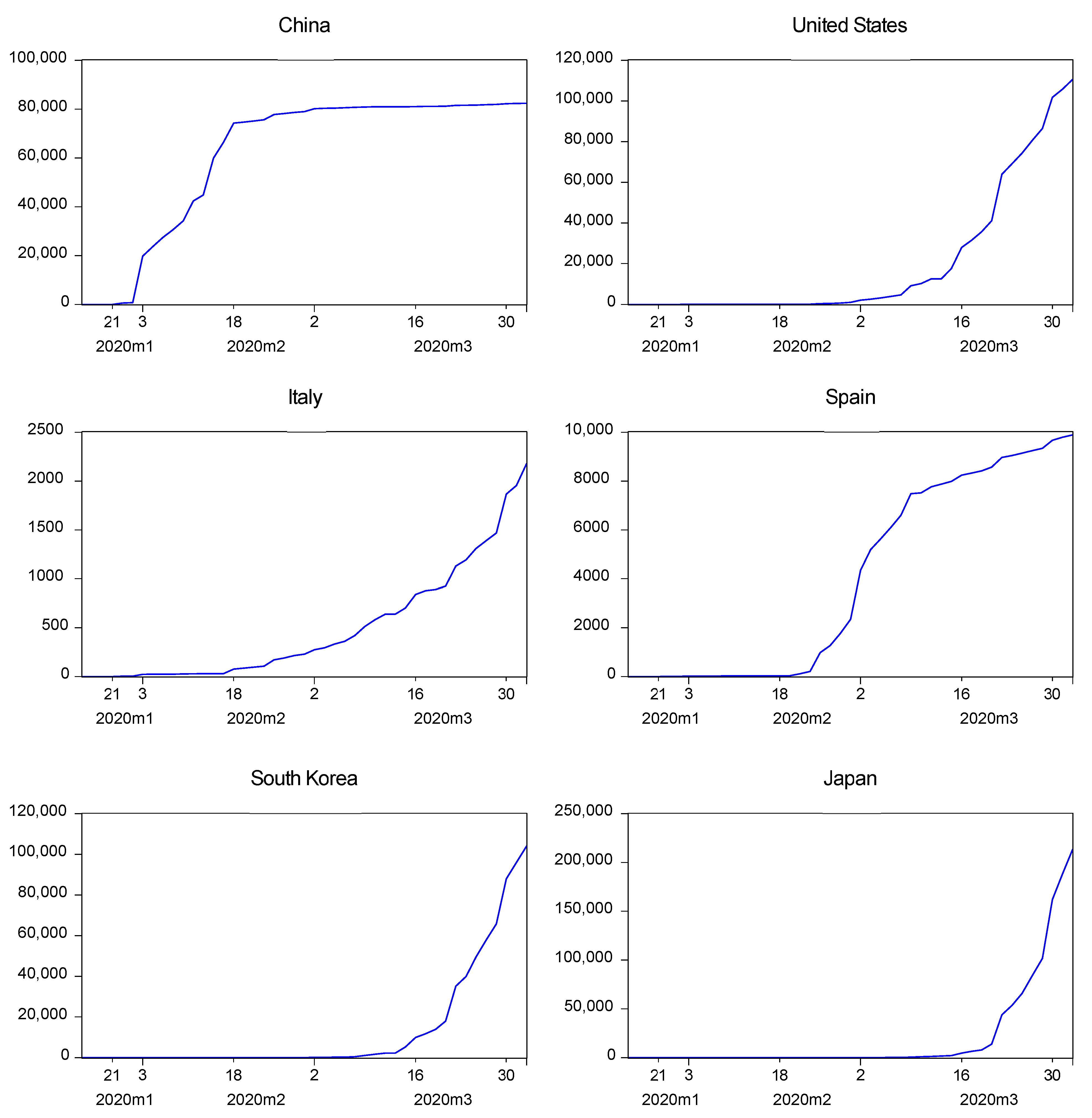
The decrease in the stock market prices corresponds with the surge in the overall number of people contaminated per day in each country (see Figure 2), where the first transmission pattern is appointed to the factor of close contact with infected individuals. The behavior of the absolute number of people infected per day in these countries suggests an inverse correlation with the stock market returns.

Figure 2. People infected per day with Covid-19. Note: M1 to M3 represents the months from January to March of 2020. The numbers in the X-axis covers the days within the months. Source: CSSE (2020).

The number of people contaminated per day is shown ahead, and the increasing trend is evident. China is considered the best performer to control the virus spread rate. The rest of the countries are struggling to keep the curve plane; however, Japan and United States have the largest contamination speed considering that the outbreak on a large scale started in February (even when the first case was detected earlier).

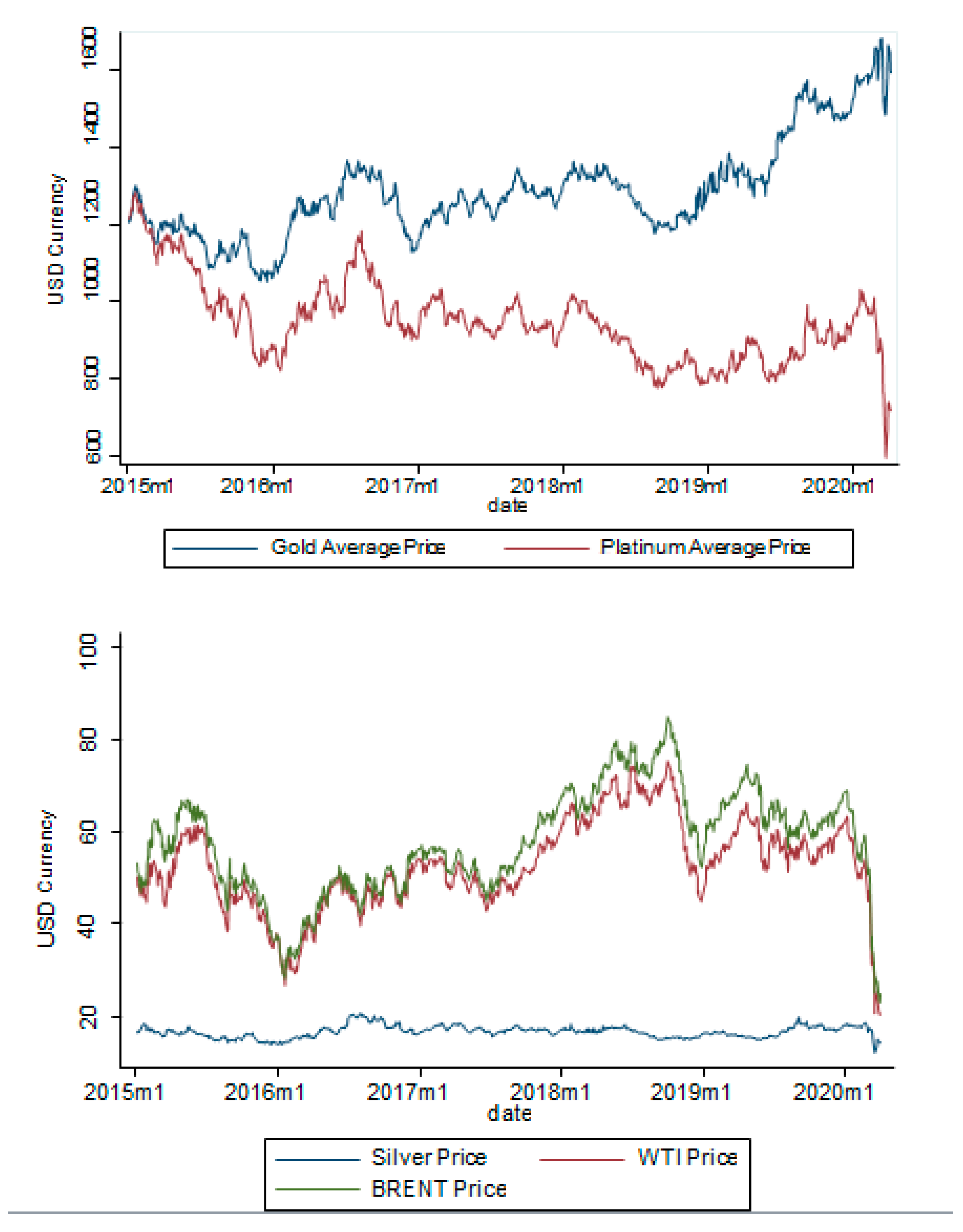
Since the financial market is closely linked with the commodity market and the overall economic production, the prices (as a measure of value) of the commodities are also influenced by COVID 19. In January 2020, it can be seen from Figure 3, that a significant prices’ drop-down started to appear with the outbreak of coronavirus across countries and it was more intense for the commodities of Gold, Platinum (measured in 1 troy ounce for each), Brent and WTI crude oil (measured in 1 barrel of oil).

Figure 3. Commodity Price Behavior. Source: Data Stream (2020).

A correlation analysis (see Table 1) measuring growth as percentage change using log-differences of these variables suggest that the contamination growth rate of Covid-19 is statistically significant and negatively correlated with the performance of the stock markets and the commodity prices, except for exchange rate and gold prices1. The highest negative correlation coefficients of the contamination growth rate of Covid-19 are with the price of the Brent oil barrel and the stock market performance.

Table 1. Correlation Matrix.

Variables	(1)	(2)	(3)	(4)	(5)	(6)	(7)	(8)
(1) Stock Market Performance	1.000	−0.120 ***	−0.002	−0.060 ***	0.093 ***	0.197 ***	0.232 ***	0.247 ***
(2) Contamination G. R.	−0.120 ***	1.000	0.002	0.004	−0.087 ***	−0.058 ***	−0.085 ***	−0.124 ***
(3) Exchange Rate G. R.	−0.002	0.002	1.000	0.120 ***	0.099 ***	0.131 ***	0.034 ***	0.028 **
(4) Gold Price G. R.	−0.060 ***	0.004	0.120 ***	1.000	0.571 ***	0.488 ***	0.049 ***	0.027 **
(5) Silver Price G. R	0.093 ***	−0.087 ***	0.099 ***	0.571 ***	1.000	0.527 ***	0.206 ***	0.196 ***
(6) Platinum Price G. R	0.197 ***	−0.058 ***	0.131 ***	0.488 ***	0.527 ***	1.000	0.214 ***	0.228 ***
(7) WTI Price G. R	0.232 ***	−0.085 ***	0.034 ***	0.049 ***	0.206 ***	0.214 ***	1.000	0.915 ***
(8) BRENT Change	0.247 ***	−0.124 ***	0.028 **	0.027 **	0.196 ***	0.228 ***	0.915 ***	1.000

Note: Pair-wise correlation coefficients are presented in the table. P-values *** p < 0.01, ** p < 0.05, significance levels Source: Own Elaboration.

Average positive returns from the stock markets of Japan, the United States, China, South Korea, Spain, and Italy are reported in Table 2 during the period between 2015 and 2020. The average number of people contaminated per day is 21,002 for all of these countries. The prices of gold and silver have an average growth of 0.016% and 0.129%, respectively. The prices of platinum, WTI, and Brent oil are decreasing during the same period. The price of the oil Brent barrel has the highest volatility, while the exchange rate has the lowest volatility. The selected stock markets for each of these countries exhibit positive returns except for Spain (see Table 3). China (FTSE China A50) has a higher return on average than the United States (Dow Jones) from 2015 to 2020.

Table 2. Descriptive Statistics.

Variable	Obs	Mean	Std.Dev.	Min	Max
Stock Market Performance	6798	0.0001105	0.013	−0.169	0.114
# of People contaminated per day *	258	21,002.61	36,291.3	0	213,372
Exchange Rate G. R.	6798	0.0000168	0.008	−0.111	0.125
Gold Price G. R	6798	0.0001613	0.01	−0.046	0.058
Silver Price G. R	6798	0.0012936	0.018	−0.136	0.076
Platinum Price G. R	6798	−0.0001951	0.014	−0.121	0.104
WTI Price G. R	6798	−0.0002151	0.027	−0.246	0.238
BRENT Change	6798	−0.0001893	0.025	−0.241	0.144

Note: The period of these descriptive statistics except the # of People contaminated per day is from the 1st of January of 2015 to the 1st of April of 2020. * The statistics associated with the infections are derived from the first reported case in the data of CSSE. Source: Own Elaboration.

Table 3. Basic statistics by country.

Country	Total Infections/Population	Statistic	Number of People Contaminated Per Day	Stock Market Performance (Returns)	Exchange Rate G.R.
China		Mean	63,934.72	0.0003436	−0.0001023
	0.19%	Minimum	0	−0.0899	−0.018
		Maximum	82,361	0.0707	0.0111
		Std. Dev.	27,530.32	0.015367	0.0024559
Italy		Mean	21,146.79	0.0000781	−0.0000218
	1.50%	Minimum	0	−0.1692	−0.0239
		Maximum	110,574	0.0893	0.0307
		Std. Dev.	33,990.32	0.0152327	0.0054836
Japan		Mean	514.9535	0.0001076	0.0001546
	0.02%	Minimum	0	−0.0792	−0.0318
		Maximum	2178	0.0804	0.0333
		Std. Dev.	596.0662	0.0129665	0.0062192
South Korea		Mean	4230.558	0.0000217	0.0000414
	0.35%	Minimum	0	−0.0839	−0.1111
		Maximum	9887	0.086	0.125
		Std. Dev.	4033.996	0.009589	0.0158595
Spain		Mean	14,032.74	−0.0001861	−0.0000218
	1.29%	Minimum	0	−0.1406	−0.0239
		Maximum	104,118	0.0782	0.0307
		Std. Dev.	28,047.99	0.0130819	0.0054836
USA		Mean	22,155.88	0.0002982	0.0000507
	0.29%	Minimum	0	−0.1293	−0.0295
		Maximum	213,372	0.1137	0.0246
		Std. Dev.	51,832.97	0.0121533	0.0054717
Total		Mean	21,002.61	0.0001105	0.0000168
	0.26%	Minimum	0	−0.1692	−0.1111
		Maximum	213,372	0.1137	0.125
		Std. Dev.	36,291.3	0.0132068	0.0080215

Note: The period of these descriptive statistics is from 1st of January of 2015 to the 1st of April of 2020 except for the number of people contaminated per day. Statistics are sourced calculated from the first reported case of the data of CSSE. All exchange rates are estimated relative to the USD. In the case of the USA exchange rate, it is measured in nominal terms of the Euro. Source: Own Elaboration.

4. Methodology

We utilize a k-variate panel VAR of order $p$ to empirically investigate the impact of the contamination rate of COVID 19 on stock market returns of first-affected countries. Following the description of Abrigo and Love (2016), the general model specification is expressed as follows:

$$\begin{array}{c}{Y}_{\mathit{i}\mathit{t}}={\displaystyle {\displaystyle \sum }_{\mathit{\gamma }=\mathbf{1}}^{\mathit{p}}}{Y}_{\mathit{i}\mathit{t}-\mathit{\gamma }}{A}_{\mathit{\gamma }}+X_{\mathit{i}\mathit{t}}B+u_{\mathit{i}}+e_{it}\\ \mathit{i}\in \left\{\mathbf{1}, 2, \dots , \mathit{N}\right\}, \mathit{t}\in \left\{\mathbf{1}, \mathbf{2}, \dots , {\mathit{T}}_{\mathit{i}}\right\}\end{array}$$

(1)

where $Y_{it}$ is a (1 × k) vector of the dependent stationary variables, which includes the performance of the stock market of country i at time t as the variable of interest, and later a set of endogenous regressors which includes the growth rate of the current exchange rates of country i at time t, the growth rate of the prices of commodities of gold, platinum, silver, WTI & BRENT oil. We assume parameter homogeneity for $A_{\gamma }\left(k \times k\right)$ and $B$ which is a matrix of $\left(l \times k\right)$ of parameters.

$X_{it}$ is the (1 × l) vector of exogenous covariates, which includes the growth rate of contagious per day of COVID 192, among this exogenous variable, the fixed effects are captured in ${\mathit{u}}_i$.

From (1) by defining $Y_{it}=\mathbf{\left[}{y}_{it}^{\mathbf{1}\mathbf{*}}\dots y_{it}^{k\mathbf{*}} \mathbf{\right]}$ as the vector of k endogenous dependent variables with $\widetilde{Z_{\mathit{i}\mathit{t}}}=\mathbf{\left[}{Y}_{\mathit{i}\mathit{t}-\mathbf{1}} \dots Y_{\mathit{i}\mathit{t}-\mathit{p}} X_{\mathit{i}\mathit{t}} \mathbf{\right]}$, which contains the autoregressive lag orders of the endogenous and exogenous variables. The matrix of coefficients is defined by $A{}^{\prime }=\mathbf{\left[}{A}_1^{{}^{\prime }} \dots A_p^{{}^{\prime }} B^{\prime } \mathbf{\right]}$ and the least-squares estimator from this panel data structure is given by $A={\mathbf{\left(}\tilde{Z}{}^{\prime }\tilde{Z}\mathbf{\right)}}^{-\mathbf{1}}\mathbf{\left(}\tilde{Z}{}^{\prime }Y\mathbf{\right)}$ which is the result of minimizing the sums of squares of the vector $e_{it}=\mathbf{\left[}{e}_{it}^{\mathbf{1}\mathbf{*}}\dots e_{it}^{k\mathbf{*}}\mathbf{\right]}$. We use the log-returns and log growth rates of all the variables to provide better economic inferences.

The performance (or returns) of the stock market which is the main variable of interest is given as

$$\mathit{r}=\frac{{\mathit{s}}_{\mathit{i}\mathit{t}+\mathit{1}}-{\mathit{s}}_{\mathit{i}\mathit{t}}}{{\mathit{s}}_{\mathit{i}\mathit{t}}}\approx \mathbf{ln}\left(\frac{{\mathit{s}}_{\mathit{i}\mathit{t}+\mathbf{1}}}{{\mathit{s}}_{\mathit{i}\mathit{t}}}\right)$$

(2)

where for country i at day t the closing stock price is represented in $s$, and it would be assumed as the growth rate of the last price registered of the stock market, equivalent to the difference in natural logarithms. Similarly, the same idea is used for the growth rates of the current exchange rate for the countries of analysis and the prices of the commodities. We use daily stock market data from China, the United States, Italy, Spain, South Korea, and Japan during the period from the 1st of January of 2015 to the 1st of April of 2020 (Datastream 2020).

Table 4 presents the stock markets used in the analysis. They are selected based on having the highest index value by each country:

Table 4. Selected stock markets.

ID	Country of Analysis	Stock Market
1	China	FTSE China A50
2	United States	DOW JONES
3	Italy	FTSE MIB
4	Spain	IBEX 35
5	South Korea	KOSPI KS11
6	Japan	NIKKEI 225 (N225)

Source: Own Elaboration.

The information regarding the number of people infected per day in each of these countries was collected from the Center for Systems Science and Engineering (CSSE) of the John Hopkins Whiting School of Engineering (CSSE 2020). CSSE provides well-documented data on the positive cases in absolute values of the population contaminated3 for all of the countries of the world.

As we are working with financial data, problems of highly persistent serial correlation and heteroskedasticity are possible. To account for these issues and to provide robustness checks for the estimations, the following methodologies are utilized4: (1) The overall panel VAR will be estimated using the panel least squares method and then compared with the Maximum Likelihood approach using the standard normal density function. (2) White–Arellano estimator (White 1980, 1984; Arellano 1987) with cross-section weights and Driscoll and Kraay (2006) robust standard errors both are used to account for heteroskedasticity and serially correlated errors5. These robust standard errors are proper in the context of our data structure that has a longer time dimension relative to panel groups (T > N) and considering the heteroskedastic, cross-sectionally dependent, and autocorrelated error structure (Hoechle 2007)6. As a VAR model is, in essence, a Seemly Unrelated Regression (SUR) model (Triacca 2014), we can follow Woolridge’s (2002) recommendation to use the generalized least square method to estimate (1). By doing this, we improve the efficiency of the results unlike using conventional OLS.

The advantage of the SUR estimation is that the correlation between the errors of the equations in (1) can be examined with the Breusch and Pagan Lagrange Multiplier (Breusch and Pagan 1980) test. De Hoyos and Sarafidis (2006) recommend this test to confirm the presence of cross-sectional dependence in the context of large panels (T > N). Based on the test results, we can confirm if Driscoll–Kraay’s robust standard errors outperform the other estimations, resulting in consistent results that account for serial correlation, heteroskedasticity, and cross-sectional dependence (Hoechle 2007).

The methodology involves confirming the property of stationarity among the variables with the first generation of panel unit-roots, considering the test of Levin et al. (2002). The second-generation tests are also performed using the ones proposed by Im et al. (2003) and the Fisher-type unit-root test (Choi 2001). For Equation (1) panel VAR with the generalized method of moments (GMM) becomes unfeasible7 for the scale of T. Nevertheless, the approximation in (1) has the same structure compared with the original panel VAR model proposed by Abrigo and Love (2016) where the model accounts for the effects with fixed individual effects, but with the explicit difference that we are working with a large scale of T in comparison to N units.

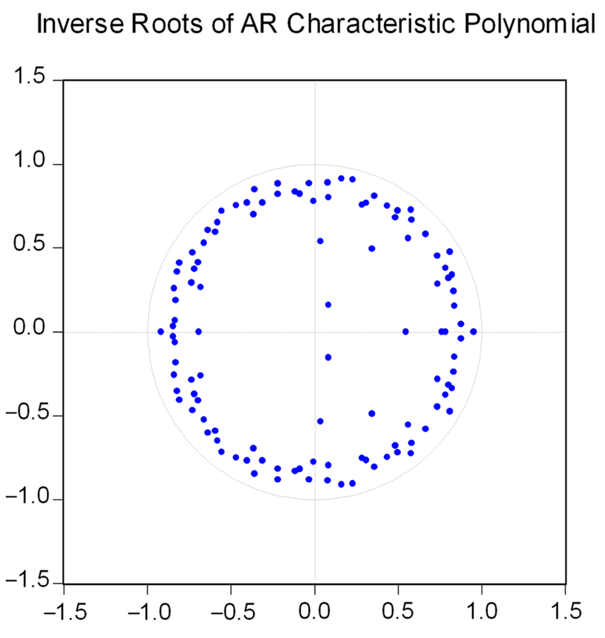
The lag selection for$p$ in Equation (1) is a problematic issue since the available literature cannot provide a proper guide for the same type of application, threatening the feasibility to perform the optimal moment and model selection criteria (MMSC) of Andrews and Lu (2001). The number of lags in $p$ is selected based on two criteria: (1) using sufficient lags to capture the persistent serial correlation in time and (2) fulfilling the condition of stability of the model regarding the autoregressive coefficients. This is considered since with too many lags, the inverse roots of the AR characteristic polynomial can shift outside the unit circle and become unstable, the concept of parsimony is imperative in this selection.

An advantage with the current structure of the data is that endogeneity bias which emerges due to the correlation of the unobserved heterogeneity and the lagged values of the dependent variable can be corrected with the fixed effects approach. Wherein as $T\to \infty$, the average error term becomes close to zero, therefore the bias induced in the dynamic panel data models can be avoided as recommended by Beck and Katz (1995).

5. Results

The first and second generation of panel unit-root tests confirmed the stationarity of the stock market performance, the growth rates of the exchange rate, the growth in the commodity prices of gold, platinum, silver, WTI, and Brent (see Appendix A). An ideal number of lags were selected based on the error criteria of AIC, BIC, FPS, and Hannan–Quinn of the VAR model8.

The overall panel least squares VAR estimation and the Maximum Likelihood approach yield identical results, which indicates a negative impact of 2.3% on the performance of the stock markets when the virus contamination rate increases by 1% across countries at the 99% confidence level. The model’s stability test is satisfactory but the Breush–Pagan Lagrange Multiplier test results report the presence of autocorrelation in the residuals. To account for this problem, the White–Arellano period estimator with cross-sectional weights, SUR, and the Driscoll–Kraay approaches were utilized. The results however remain robust, a decrease of around 2.3% of the performance of the stock markets is explained by the Corona Virus contamination. A slight reduction in the magnitude of the stock market performance variable to 2.1% is observed with the White–Arellano estimator (see Appendix B for all the regression outputs).

According to the SUR model, the Breusch–Pagan test of independence is rejected, indicating the presence of cross-sectional dependence in the model of Equation (1), therefore, the Driscoll–Kraay approach provides the most accurate results as it accounts for the problems of serial correlation, heteroskedasticity, and cross-sectional dependence. The results from this approach are consistent with the rest of the estimations, yielding an empirical finding of a negative impact of 2.3% in the stock market performance across countries in time, significant at the 99% confidence level ceteris paribus.

The coronavirus is not statistically significant to explain the changes in the exchange rate and the growth of the prices of gold in the countries of analysis, regardless of this result, it is significant at the 90% confidence level to explain changes related to the prices of platinum, silver, WTI, and Brent crude oil. By a 1% increase of the coronavirus contamination rate, a significant reduction of 1.1%, 1.6%, 3.26%, and 4.08% in the prices of platinum, silver, WTI, and Brent occur. It can be noted that the biggest drop is associated with the Brent oil price, similar to Bakas and Triantafyllou (2020) results.

Empirical findings regarding the Granger-causality tests derived from the Driscoll–Kraay approach are located in Appendix C. Considering the transformation of all of the variables in growth rates related to the closing prices, these tests allow to enhance the understanding of the model inner dynamics, and permits a differential view of the propensities among the correlations between the variables. The results are as follows: (1) Exchange rate, platinum, and gold granger cause the stock market performance. (2) Stock market performance, platinum, and gold granger cause exchange rate. (3) WTI, exchange rate, and oil granger cause gold. (4) Brent, WTI, and gold and silver granger cause platinum. (5) Exchange rate, Brent, WTI, Gold, and platinum granger cause silver. (6) Silver is the only variable that granger causes WTI, and Brent is granger-caused by the exchange rate. It is important to note that these dynamics are observed only during the period from January of 2015 to April of 2020, therefore, possible market deviations or new intercorrelations might arise in the future as the coronavirus endure.

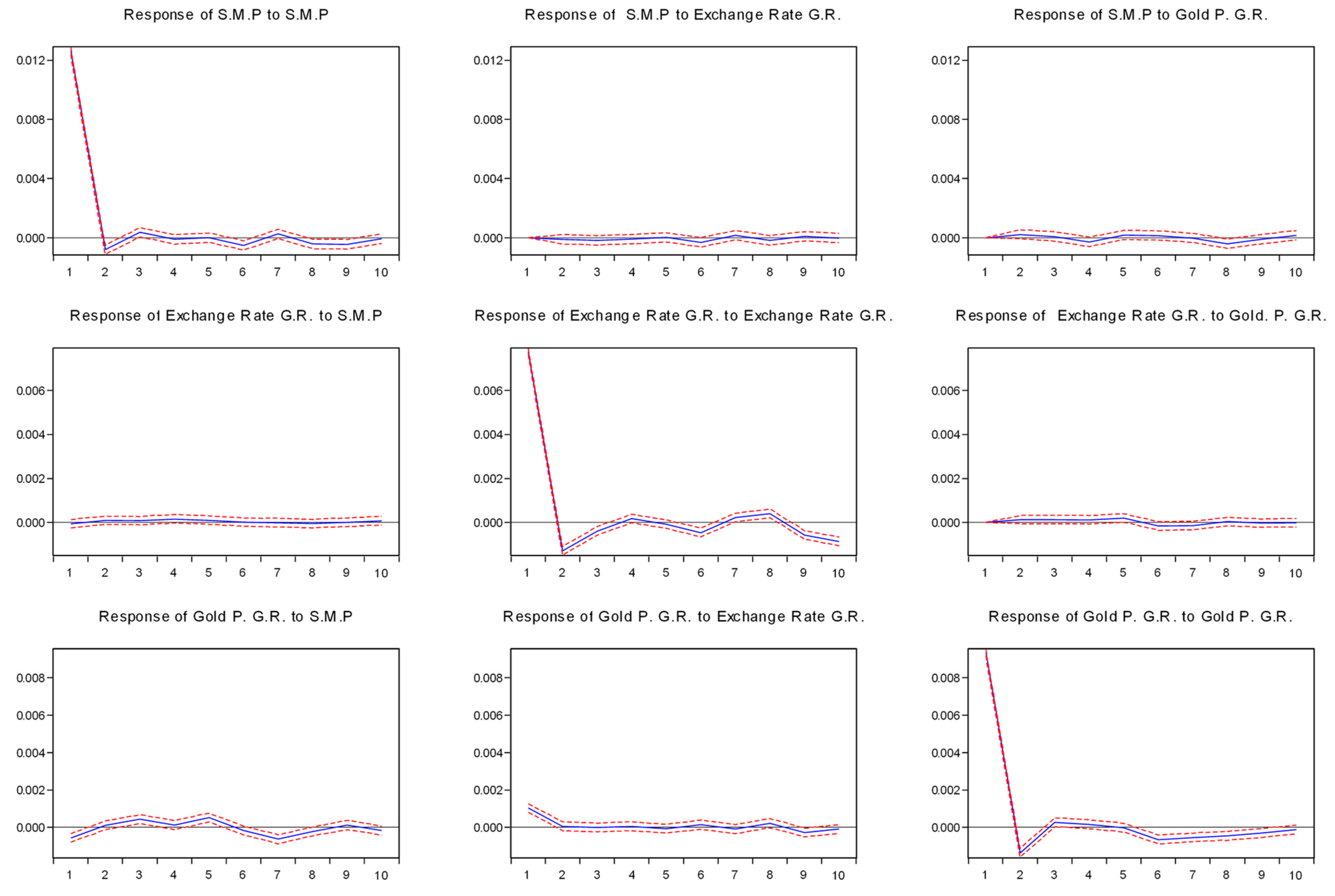
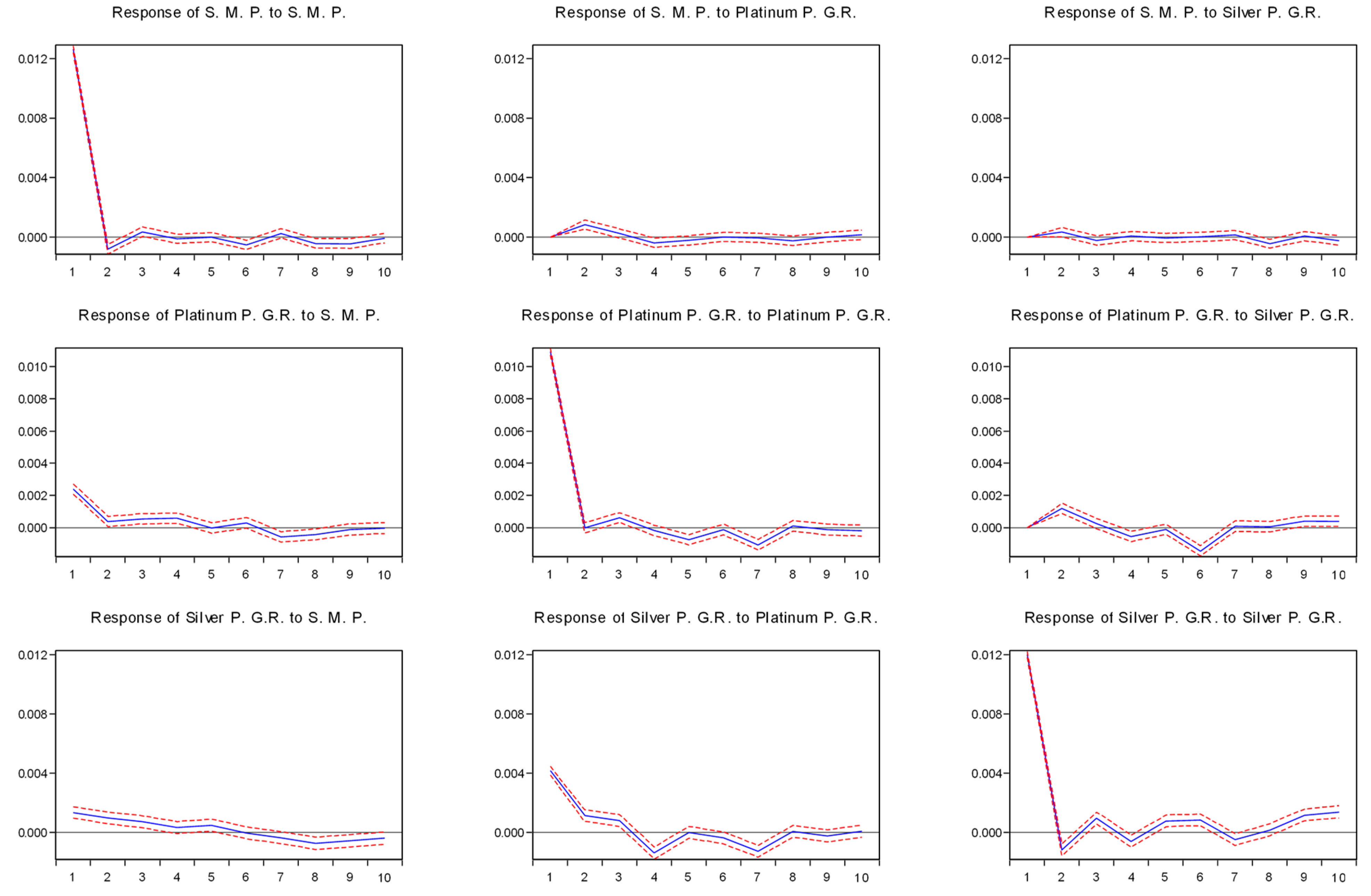
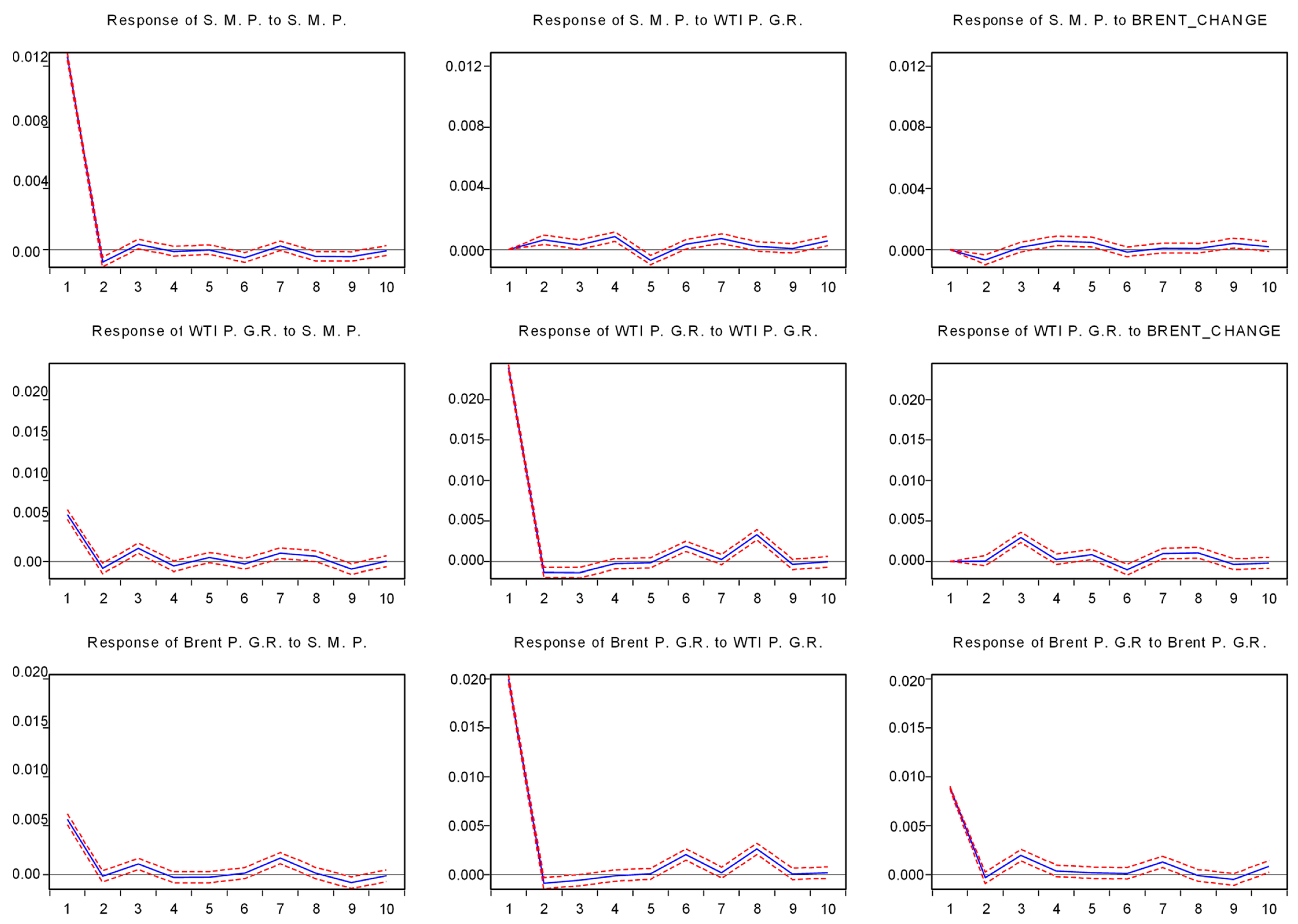
The impulse response function of the panel VAR model is presented in Appendix D, and it indicates that within an initial shock, for each variable considering the response for its own, there’s a decreasing but significant effect, which tends to disappear in 8–10 days. A positive shock in stock market performance causes a short-termed positive shock in gold, WTI, and Brent oil. Platinum and silver commodities tend to behave similarly yet for a relatively long period, around 4 days after initial shock in the stock market performance. A positive shock in Brent tends to increase WTI prices. Silver reacts positively to stock market performance for a short time, then the effect reverts after the fifth day and becomes negative.

6. Conclusions

This research empirically quantifies the negative impact of the coronavirus on the stock market performance in China, the United States, Italy, South Korea, Spain, and Japan. The results across the different estimations suggest that a 1% increase in the virus contamination rate, reduces stock market returns by 2.3% on daily basis. The negative impact of the Coronavirus contamination extends to adversely influence the prices of global commodities like platinum, silver, Brent and WTI oil. The largest drop is observed in oil barrel prices, wherein an increase in the virus spread rate causes a decline of 4.08% and 3.26% in Brent and WTI oil prices respectively. These results reflect the state of global stagnation as well the severe changes in individual and institutional supply and demand behavior as the Virus hit the world. The oil price dropdown cannot be solely explained by the Coronavirus-related induced reduction in global demand, the ”Oil Price War” between Saudi Arabia and Russia also contributes to pushing down and destabilize the oil prices (Cohen 2020). With the pandemic yet on the rise and the death toll has not ended, any economic analysis or projection for the long-term effects of the virus on the stock market is subject to uncertainty. Further market disruptions are anticipated, institutions and individuals are, and will continue, experiencing liquidity stress that stimulates the demand for corporate and private debt. The drop in the demand and supply of global commodities is lower relative to the oil drop, but as the pandemic endure, severe behavioral changes by end-users will alter the global demand for commodities and industrial services. Ashraf’s (2020a) argument that the cultural risk aversion level defines the intensity of the market response to COVID 19, comes in line with our results. Market agents opt to reduce the ensued adverse effects by shifting their preferences towards safer investment heavens. This explains the sluggish and non-significant COVID 19 impact on gold and exchange rate in our results relative to the conventional stock market portfolios.

References

- Abrigo, Michael R., and Inessa Love. 2016. Estimation of panel vector autoregression in Stata. The Stata Journal 16: 778–804. [Google Scholar] [CrossRef]
- Albulesco, Claudiu Tiberiu. 2020. COVID-19 and the United States financial markets’ volatility. Finance Research Letters. in press. [Google Scholar] [CrossRef]
- Albuquerque, Rui, Yrjo Koskinen, and Chendi Zhang. 2019. Corporate social responsibility and firm risk: Theory and empirical evidence. Management Science 65: 4451–69. [Google Scholar] [CrossRef]
- Albuquerque, Rui, Yrjo Koskinen, Shuai Yang, and Chendi Zhang. 2020. Resiliency of environmental and social stocks: An analysis of the exogenous Covid-19 market crash. The Review of Corporate Finance Studies 9: 593–621, ECGI paper No. 676. [Google Scholar] [CrossRef]
- Andrews, Donald Wilfrid Kao, and Biao Lu. 2001. Consistent model and moment selection procedures for GMM estimation with application to dynamic panel data models. Journal of Econometrics 101: 123–64. [Google Scholar] [CrossRef]
- Arellano, Manuel. 1987. Practitioners’ corner: Computing robust standard errors for within-groups estimators. Oxford Bulletin of Economics & Statistics 49: 431–34. [Google Scholar]
- Ashraf, Badar Nadeem. 2020a. Stock markets’ reaction to Covid-19: Moderating role of national culture. Finance Research Letter. [Google Scholar] [CrossRef]
- Ashraf, Badar Nadeem. 2020b. Stock markets’ reaction to COVID-19: Cases or fatalities. Research in International Business and Finance 54: 101249. [Google Scholar] [CrossRef]
- Bakas, Dimitrios, and Athanasios Triantafyllou. 2020. Commodity price volatility and the economic uncertainty of pandemic. Economic Letters 193: 109283. [Google Scholar] [CrossRef]
- Baker, Scott R., Nicholas Bloom, Steven J. Davis, Kyle J. Kost, Marco C. Sammon, and Tasaneeya Viratyosin. 2020. The Unprecedented Stock Market Impact of COVID-19. NBER Working Paper No. 26954. Cambridge: National Bureau of Economic Research, Inc. [Google Scholar]
- Barro, Robert, José F. Ursua, and Joanna Weng. 2020. The Coronavirus and the Great Influenza Pandemic: Lessons from the “Spanish Flu” for the Coronavirus’s Potential Effects on Mortality and Economic Activity. NBER Working Paper No. 26866. Cambridge: National Bureau of Economic Research, Inc. [Google Scholar]
- Beck, Nathaniel, and Jonathan Katz. 1995. What to do (and not to do) with time-series cross-section data. The American Political Science Review 89: 634–47. [Google Scholar] [CrossRef]
- Bell, Clive, and Maureen Lewis. 2004. The Economic Implications of Epidemics Old and New. World Economics 5: 137–74. [Google Scholar]
- Benmelech, Efraim, and Carola Frydman. 2020. The 1918 Influenza Did Not Kill the US Economy. Retrieved from VOXEU. Available online: https://voxeu.org/article/1918-influenza-did-not-kill-us-economy (accessed on 12 July 2020).
- Brainerd, Elizabeth, and Mark Siegler. 2003. The Economic Effects of the 1918 Influenza Epidemic. CEPR Discussion Paper No. 3791. London: Centre for Economic Policy Research. [Google Scholar]
- Breusch, Trevor Stanley, and Adrian Rodney Pagan. 1980. The Lagrange multiplier test and its applications to model specification in econometrics. Review of Economic Studies 47: 239–53. [Google Scholar] [CrossRef]
- Capelle-Blancard, G., and A. Desroziers. 2020. The Stock Market Is Not The Economy? Insights From The COVID-19 Crisis. Covid Economics: Vetted and Real-Time Papers. London: CEPR Centre for Economic Policy Research. [Google Scholar]
- CDC. 2004. SARS (10 Years After). Retrieved from Centers for Diesease Cintrol and Prevention. Available online: https://www.cdc.gov/dotw/sars/index.html (accessed on 27 June 2020).
- CDC. 2019. Ten Years of Gains: A Look Back at Progress since the 2009 H1N1 Pandemic. Retrieved from Centers for Diesease Cintrol and Prevention. Available online: https://www.cdc.gov/flu/spotlights/2018-2019/decade-since-h1n1-pandemic.html (accessed on 25 June 2020).
- Choi, In. 2001. Unit root tests for panel data. Journal of International Money and Finance 20: 249–72. [Google Scholar] [CrossRef]
- Cohen, Ariel. 2020. Too Little too Late? Russia and Saudi Arabia Reach Truce in Oil Price War. Retrived from Forbes. Available online: https://bit.ly/2W9STZC (accessed on 20 April 2020).
- Correia, Sergio, Stephan Luck, and Emil Verner. 2020. Pandemics Depress the Economy, Public Health Interventions Do Not: Evidence from the 1918 Flu. Available online: https://ssrn.com/abstract=3561560 (accessed on 5 June 2020).
- CSSE. 2020. Time-Series Covid19 Confirmed Global Cases. Retrieved from Center for Systems Science and Engineering. John Hopkins Whiting School of Engineering, John Hopkins, Baltimore. Available online: https://bit.ly/3j3Qzxt (accessed on 20 April 2020).
- Datastream. 2020. Datastream International. Available online: https://libguides.princeton.edu/datastream/ (accessed on 20 April 2020).
- De Hoyos, Rafael, and Vasilis Sarafidis. 2006. Testing for cross-sectional dependence in panel-data models. The Stata Journal 6: 482–96. [Google Scholar] [CrossRef]
- Driscoll, John C., and Aart C. Kraay. 2006. Consistent covariance matrix estimation with spatially dependent panel data. Review of Economics and Statistics 80: 549–60. [Google Scholar] [CrossRef]
- Engelhardt, Nils, Miguel Krause, Daniel Neukirchen, and Peter N. Posch. 2020. Trust and stock market volatility during the COVID-19 crisis. Finance Research Letters. [Google Scholar] [CrossRef]
- Gormsen, Niels Joachim, and Ralph S. J. Koijen. 2020. Coronavirus: Impact On Stock Prices And Growth Expectations. NBER Working Paper No. 27387. Cambridge: National Bureau of Economic Research, Inc. [Google Scholar]
- He, Qing, Junyi Liu, Sizhu Wang, and Jishuang Yu. 2020. The impact of COVID-19 on stock markets. Economic and Political Studies. [Google Scholar] [CrossRef]
- Hoechle, Daniel. 2007. Robust standard errors for panel regressions with cross-sectional dependence. The Stata Journal 7: 281–312. [Google Scholar] [CrossRef]
- Im, Kyung So, Mohammad Pesaran, and Yongcheol Shin. 2003. Testing for unit roots in heterogeneous panels. Journal of Econometrics 115: 53–74. [Google Scholar] [CrossRef]
- Jonung, Lars, and Werner Roeger. 2006. The Macroeconomic Effects of a Pandemic in Europe—A Model-Based Assessment. European Commission Working Paper No. 251. Brussels: European Commission. [Google Scholar]
- Karlsson, Martin, Therese Nilsson, and Stefan Pichler. 2014. The impact of the 1918 Spanish flu epidemic oneconomic performance in Sweden: An investigation into the consequences of an extraordinary mortality shock. Journal of Health Economics 36: 1–19. [Google Scholar] [CrossRef]
- Levin, Andrew, Chien-Fu Lin, and Chia-Shang-James Chu. 2002. Unit root tests in panel data: Asymptotic and finite-sample properties. Journal of Econometrics 108: 1–24. [Google Scholar] [CrossRef]
- Moundigbaye, Mantobaye, William S. Rea, and W. Robert Reed. 2018. Which panel data estimator should I use?: A corrigendum and extension. Economics E-Journal 12: 1–33. [Google Scholar] [CrossRef]
- Takyi, Paul Owusu, and Isaac Bentum-Ennin. 2020. The impact of COVID-19 on stock market performance in Africa: A Bayesian structural time series approach. Journal of Economics and Business. [Google Scholar] [CrossRef] [PubMed]
- Triacca, Umberto. 2014. Lesson 17: Vector Autoregressive Models. Retrieved from Dipartimento di Ingegneria e Scienze dell’Informazione e Matematica, Universit’a dell’Aquila. Available online: http://www.phdeconomics.sssup.it/documents/Lesson17.pdf (accessed on 22 April 2020).
- Verikios, Geroge, James McCaw, Jodie McVernon, and Anthony Harris. 2012. H1N1 influenza and the Australian macroeconomy. Journal of the Asia Pacific Economy 17: 22–51. [Google Scholar] [CrossRef]
- White, Halbert. 1980. Asymptotic Theory for Econometricians. Orlando: Academic Press. [Google Scholar]
- White, Halbert. 1984. Heteroskedasticity–consistent covariance matrix and a direct test for heteroskedasticity. Econometrica 48: 817–38. [Google Scholar] [CrossRef]
- WHO. 2012. Middle East Respiratory Syndrome Coronavirus (MERS-CoV). Retrieved from World Health Organization. Available online: https://www.who.int/emergencies/mers-cov/en/ (accessed on 12 July 2020).
- WHO. 2020. Coronavirus Disease (COVID-19) Pandemic. Retrieved from World Health Organization. Available online: https://www.who.int/emergencies/diseases/novel-coronavirus-2019 (accessed on 12 July 2020).
- Woolridge, J. 2002. Econometric Analysis of Cross Section and Panel Data. Cambridge: The MIT Press. [Google Scholar]
- World Bank 2016. 2014–2015 West Africa Ebola Crisis: Impact Update. Retrieved from World Bank. Available online: https://www.worldbank.org/en/topic/macroeconomics/publication/2014-2015-west-africa-ebola-crisis-impact-update (accessed on 22 June 2020).
- Young, Alwyn. 2005. The gift of the dying: The tragedy of Aids and the welfare of future African generations. The Quarterly Journal of Economics 120: 423–66. [Google Scholar]
- Zhang, Dayong, Min Hu, and Qiang Ji. 2020. Financial markets under the global pandemic of COVID-19. Finance Research Letter. [Google Scholar] [CrossRef]