Pricing and Hedging American-Style Options with Deep Learning

Abstract

In this paper we introduce a deep learning method for pricing and hedging American-style options. It first computes a candidate optimal stopping policy. From there it derives a lower bound for the price. Then it calculates an upper bound, a point estimate and confidence intervals. Finally, it constructs an approximate dynamic hedging strategy. We test the approach on different specifications of a Bermudan max-call option. In all cases it produces highly accurate prices and dynamic hedging strategies with small replication errors.

1. Introduction

Early exercise options are notoriously difficult to value. For up to three underlying risk factors, tree based and classical PDE approximation methods usually yield good numerical results; see, e.g., Forsyth and Vetzal (2002); Hull (2003); Reisinger and Witte (2012) and the references therein. To treat higher-dimensional problems, various simulation based methods have been developed; see, e.g., Tilley (1993); Barraquand and Martineau (1995); Carriere (1996); Andersen (2000); Longstaff and Schwartz (2001); Tsitsiklis and Van Roy (2001); García (2003); Broadie and Glasserman (2004); Bally et al. (2005); Kolodko and Schoenmakers (2006); Egloff et al. (2007); Broadie and Cao (2008); Berridge and Schumacher (2008); Jain and Oosterlee (2015). Haugh and Kogan (2004) as well as Kohler et al. (2010) have already used shallow1 neural networks to estimate continuation values. More recently, in Sirignano and Spiliopoulos (2018) optimal stopping problems in continuous time have been solved by approximating the solutions of the corresponding free boundary PDEs with deep neural networks. In Becker et al. (2019a, 2019b), deep learning has been used to directly learn optimal stopping strategies. The main focus of these papers is to derive optimal stopping rules and accurate price estimates.

The goal of this article is to develop a deep learning method which learns the optimal exercise behavior, prices and hedging strategies from samples of the underlying risk factors. It first learns a candidate optimal stopping strategy by regressing continuation values on multilayer neural networks. Employing the learned stopping strategy on a new set of Monte Carlo samples gives a low-biased estimate of the price. Moreover, the candidate optimal stopping strategy can be used to construct an approximate solution to the dual martingale problem introduced by Rogers (2002) and Haugh and Kogan (2004), yielding a high-biased estimate and confidence intervals for the price. In the last step, our method learns a dynamic hedging strategy in the spirit of Han et al. (2018) and Buehler et al. (2019). However, here, the continuation value approximations learned during the construction of the optimal stopping strategy can be used to break the hedging problem down into a sequence of smaller problems that learn the hedging portfolio only from one possible exercise date to the next. Alternative ways of computing hedging strategies consist in calculating sensitivities of option prices (see, e.g., Bally et al. 2005; Bouchard and Warin 2012; Jain and Oosterlee 2015) or approximating a solution to the dual martingale problem (see, e.g., Rogers 2002, 2010).

Our work is related to the preprints Lapeyre and Lelong (2019) and Chen and Wan (2019). Lapeyre and Lelong (2019) also use neural network regression to estimate continuation values. However, the networks are slightly different. While they work with leaky ReLU activation functions, we use tanh activation. Moreover, Lapeyre and Lelong (2019) study the convergence of the pricing algorithm as the number of simulations and the size of the network go to infinity, whereas we calculate a posteriori guarantees for the prices and use the estimated continuation value functions to implement efficient hedging strategies. Chen and Wan (2019) propose an alternative way of calculating prices and hedging strategies for American-style options by solving BSDEs.

The rest of the paper is organized as follows. In Section 2 we describe our neural network version of the Longstaff–Schwartz algorithm to estimate continuation values and construct a candidate optimal stopping strategy. In Section 3 the latter is used to derive lower and upper bounds as well as confidence intervals for the price. Section 4 discusses two different ways of computing dynamic hedging strategies. In Section 5 the results of the paper are applied to price and hedge a Bermudan call option on the maximum of different underlying assets. Section 6 concludes.

2. Calculating a Candidate Optimal Stopping Strategy

We consider an American-style option that can be exercised at any one of finitely2 many times $0=t_0<t_1<\cdots <t_N=T$. If exercised at time $t_n$, it yields a discounted payoff given by a square-integrable random variable $G_n$ defined on a filtered probability space $(\Omega ,\mathcal{F},\mathbb{F}={\left({\mathcal{F}}_n\right)}_{n=0}^N,\mathbb{P})$. We assume that ${\mathcal{F}}_n$ describes the information available at time $t_n$ and $G_n$ is of the form $g(n,X_n)$ for a measurable function $g:\left\{0,1,\dots ,N\right\}\times {\mathbb{R}}^d\to [0,\infty )$ and a d-dimensional $\mathbb{F}$-Markov process3 ${\left(X_n\right)}_{n=0}^N$. We assume $X_0$ to be deterministic and $\mathbb{P}$ to be the pricing measure. So that the value of the option at time 0 is given by

$$V=\underset{\tau \in \mathcal{T}}{\sup }\mathbb{E}{G}_{\tau },$$

where $\mathcal{T}$ is the set of all $\mathbb{F}$-stopping times $\tau :\Omega \to \left\{0,1,\dots ,N\right\}$. If the option has not been exercised before time $t_n$, its discounted value at that time is

$$V_{t_n}={\mathrm{ess}\sup }_{\tau \in {\mathcal{T}}_n}\mathbb{E}[G_{\tau }\mid {\mathcal{F}}_n],$$

(1)

where ${\mathcal{T}}_n$ is the set of all $\mathbb{F}$-stopping times satisfying $n\le \tau \le N$.

Obviously, ${\tau }_N\equiv N$ is optimal for $V_T=G_N$. From there, one can recursively construct the stopping times

$${\tau }_n:=\left\{\begin{array}{cc}n\hfill & \mathrm{if} G_n\ge \mathbb{E}[G_{{\tau }_{n+1}}\mid X_n]\hfill \\ {\tau }_{n+1}\hfill & \mathrm{if} G_n<\mathbb{E}[G_{{\tau }_{n+1}}\mid X_n].\hfill \end{array}\right.$$

(2)

Clearly, ${\tau }_n$ belongs to ${\mathcal{T}}_n$, and it can be checked inductively that

$$V_{t_n}=\mathbb{E}[G_{{\tau }_n}\mid {\mathcal{F}}_n]=G_n\vee \mathbb{E}[V_{t_{n+1}}\mid X_n]\mathrm{for} \mathrm{all} n\le N-1.$$

In particular, ${\tau }_n$ is an optimizer of (1).

Recursion (2) is the theoretical basis of the Longstaff and Schwartz (2001) method. Its main computational challenge is the approximation of the conditional expectations $\mathbb{E}[G_{{\tau }_{n+1}}\mid X_n]$. It is well known that $\mathbb{E}[G_{{\tau }_{n+1}}\mid X_n]$ is of the form $c\left(X_n\right)$, where $c:{\mathbb{R}}^d\to \mathbb{R}$ minimizes the mean squared distance $\mathbb{E}\left[{\left\{G_{{\tau }_{n+1}}-c\left(X_n\right)\right\}}^2\right]$ over all Borel measurable functions from ${\mathbb{R}}^d$ to $\mathbb{R}$; see, e.g., Bru and Heinich (1985). The Longstaff–Schwartz algorithm approximates $\mathbb{E}[G_{{\tau }_{n+1}}\mid X_n]$ by projecting $G_{{\tau }_{n+1}}$ on the linear span of finitely many basis functions. However, it is also possible to project on a different subset. If the subset is given by $c^{\theta }\left(X_n\right)$ for a function family $c^{\theta }:{\mathbb{R}}^d\to \mathbb{R}$ parametrized by $\theta$, one can apply the following variant4 of the Longstaff–Schwartz algorithm:

(i)

Simulate5 paths ${\left(x_n^k\right)}_{n=0}^N$, $k=1,\dots ,K$, of the underlying process ${\left(X_n\right)}_{n=0}^N$.

(ii)

Set $s_N^k\equiv N$ for all k.

(iii)

For $1\le n\le N-1$, approximate $\mathbb{E}\left[G_{{\tau }_{n+1}}\mid X_n\right]$ with $c^{{\theta }_n}\left(X_n\right)$ by minimizing the sum

$$\sum _{k=1}^K{\left(g(s_{n+1}^k,x_{s_{n+1}^k}^k)-c^{\theta }\left(x_n^k\right)\right)}^2\mathrm{over}\theta .$$

(3)

(iv)

Set

$$s_n^k:=\left\{\begin{array}{cc}n\hfill & \mathrm{if} g(n,x_n^k)\ge c^{{\theta }_n}\left(x_n^k\right)\hfill \\ s_{n+1}^k\hfill & \mathrm{otherwise}.\hfill \end{array}\right.$$

(v)

Define ${\theta }_0:=\frac{1}{K}{\sum }_{k=1}^{K}g(s_1^k,x_{s_1^k}^k)$, and set $c^{{\theta }_0}$ constantly equal to ${\theta }_0$.

In this paper we specify $c^{\theta }$ as a feedforward neural network, which in general, is of the form

$$a_I^{\theta }\circ {\phi }_{q_{I-1}}\circ a_{I-1}^{\theta }\circ \cdots \circ {\phi }_{q_1}\circ a_1^{\theta },$$

(4)

where

• $I\ge 1$ denotes the depth and $q_0,q_1,\dots ,q_I$ the numbers of nodes in the different layers;
• $a_1^{\theta }:{\mathbb{R}}^{q_0}\to {\mathbb{R}}^{q_1},\dots ,a_I^{\theta }:{\mathbb{R}}^{q_{I-1}}\to {\mathbb{R}}^{q_I}$ are affine functions;
• For $j\in \mathbb{N}$, ${\phi }_j:{\mathbb{R}}^j\to {\mathbb{R}}^j$ is of the form ${\phi }_j(x_1,\dots ,x_j)=(\phi \left(x_1\right),\dots ,\phi \left(x_j\right))$ for a given activation function $\phi :\mathbb{R}\to \mathbb{R}$.

The components of the parameter $\theta$ consist of the entries of the matrices $A_1,\dots ,A_I$ and vectors $b_1,\dots ,b_I$ appearing in the representation of the affine functions $a_i^{\theta }x=A_{i}x+b_i$, $i=1,\dots ,I$. So, $\theta$ lives in ${\mathbb{R}}^q$ for $q={\sum }_{i=1}^I{q}_i(q_{i-1}+1)$. To minimize (3) we choose a network with $q_I=1$ and employ a stochastic gradient descent method.

3. Pricing

3.1. Lower Bound

Once ${\theta }_0,{\theta }_1,\dots ,{\theta }_{N-1}$ have been determined, we set $\Theta =({\theta }_0,\dots ,{\theta }_{N-1})$ and define

$${\tau }^{\Theta }:=\min \left\{n\in \left\{0,1,\dots ,N-1\right\}:g(n,X_n)\ge c^{{\theta }_n}\left(X_n\right)\right\},\mathrm{where} \min \varnothing \mathrm{is} \mathrm{understood} \mathrm{as} N.$$

This defines a valid $\mathbb{F}$-stopping time. Therefore, $L=\mathbb{E}g({\tau }^{\Theta },X_{{\tau }^{\theta }})$ is a lower bound for the optimal value V. However, typically, it is not possible to calculate the expectation exactly. Therefore, we generate simulations $g^k$ of $g({\tau }^{\Theta },X_{{\tau }^{\Theta }})$ based on independent sample paths6 ${\left(x_n^k\right)}_{n=0}^N$, $k=K+1,\dots ,K+K_L$, of ${\left(X_n\right)}_{n=0}^N$ and approximate L with the Monte Carlo average

$$\widehat{L}=\frac{1}{K_L}\sum _{k=K+1}^{K+K_L}{g}^k.$$

Denote by $z_{\alpha /2}$ the $1-\alpha /2$ quantile of the standard normal distribution and consider the sample standard deviation

$${\widehat{\sigma }}_L=\sqrt{\frac{1}{K_L-1}\sum _{k=K+1}^{K+K_L}{\left(g^k-\widehat{L}\right)}^2}.$$

Then one obtains from the central limit theorem that

$$\left[\widehat{L}-z_{\alpha /2}\frac{{\widehat{\sigma }}_L}{\sqrt{K_L}},\infty \right)$$

(5)

is an asymptotically valid $1-\alpha /2$ confidence interval for L.

3.2. Upper Bound, Point Estimate and Confidence Intervals

Our derivation of an upper bound is based on the duality results of Rogers (2002); Haugh and Kogan (2004) and Becker et al. (2019a). By Rogers (2002) and Haugh and Kogan (2004), the optimal value V can be written as

$$V=\mathbb{E}\left[\underset{0\le n\le N}{\max }\left(G_n-M_n\right)\right],$$

where ${\left(M_n\right)}_{n=0}^N$ is the martingale part of the smallest $\mathbb{F}$-supermartingale dominating the payoff process ${\left(G_n\right)}_{n=0}^N$. We approximate ${\left(M_n\right)}_{n=0}^N$ with the $\mathbb{F}$-martingale ${\left(M_n^{\Theta }\right)}_{n=0}^N$ obtained from the stopping decisions implied by the trained continuation value functions $c^{{\theta }_n}$, $n=0,\dots ,N-1$, as in Section 3.2 of Becker et al. (2019a). We know from Proposition 7 of Becker et al. (2019a) that if ${\left({\epsilon }_n\right)}_{n=0}^N$ is a sequence of integrable random variables satisfying $\mathbb{E}\left[{\epsilon }_n\mid {\mathcal{F}}_n\right]=0$ for all $n=0,1,\dots ,N$, then

$$U=\mathbb{E}\left[\underset{0\le n\le N}{\max }\left(G_n-M_n^{\Theta }-{\epsilon }_n\right)\right]$$

is an upper bound for V. As in Becker et al. (2019a), we use nested simulation7 to generate realizations $m_n^k$ of $M_n^{\Theta }+{\epsilon }_n$ along independent realizations ${\left(x_n^k\right)}_{n=0}^N$, $k=K+K_L+1,\dots ,K+K_L+K_U$, of ${\left(X_n\right)}_{n=0}^N$ sampled independently of ${\left(x_n^k\right)}_{n=0}^N$, $k=1,\dots K$, and estimate U as

$$\widehat{U}=\frac{1}{K_U}\sum _{k=K+K_L+1}^{K+K_L+K_U}\underset{0\le n\le N}{\max }(g(n,x_n^k)-m_n^k).$$

Our point estimate of V is

$$\widehat{V}=\frac{\widehat{L}+\widehat{U}}{2}.$$

The sample standard deviation of the estimator $\widehat{U}$, given by

$${\widehat{\sigma }}_U=\sqrt{\frac{1}{K_U-1}\sum _{k=K+K_L+1}^{K+K_L+K_U}{\left(\underset{0\le n\le N}{\max }(g(n,x_n^k)-m_n^k)-\widehat{U}\right)}^2},$$

can be used together with the one-sided confidence interval (5) to construct the asymptotically valid two-sided $1-\alpha$ confidence interval

$$\left[\widehat{L}-z_{\alpha /2}\frac{{\widehat{\sigma }}_L}{\sqrt{K_L}},\widehat{U}+z_{\alpha /2}\frac{{\widehat{\sigma }}_U}{\sqrt{K_U}}\right]$$

(6)

for the true value V; see Section 3.3 of Becker et al. (2019a).

4. Hedging

We now consider a savings account together with $e\in \mathbb{N}$ financial securities as hedging instruments. We fix a positive integer M and introduce a time grid $0=u_1<u_2<\cdots <u_{NM}$ such that $u_{nM}=t_n$ for all $n=0,1,\dots ,N$. We suppose that the information available at time $u_m$ is described by ${\mathcal{H}}_m$, where $\mathbb{H}={\left({\mathcal{H}}_m\right)}_{m=0}^{MN}$ is a filtration satisfying ${\mathcal{H}}_{nM}={\mathcal{F}}_n$ for all n. If any of the financial securities pay dividends, they are immediately reinvested. We assume that the resulting discounted8 value processes are of the form $P_{u_m}=p_m\left(Y_m\right)$ for measurable functions $p_m:{\mathbb{R}}^d\to {\mathbb{R}}^e$ and an $\mathbb{H}$-Markov process9 ${\left(Y_m\right)}_{m=0}^{NM}$ such that $Y_{nM}=X_n$ for all $n=0,\dots ,N$. A hedging strategy consists of a sequence $h={\left(h_m\right)}_{m=0}^{NM-1}$ of functions $h_m:{\mathbb{R}}^d\to {\mathbb{R}}^e$ specifying the time-$u_m$ holdings in $P_{u_m}^1,\dots ,P_{u_m}^e$. As usual, money is dynamically deposited in or borrowed from the savings account to make the strategy self-financing. The resulting discounted gains at time $u_m$ are given by

$${(h·P)}_{u_m}:=\sum _{j=0}^{m-1}{h}_j\left(Y_j\right)·\left(p_{j+1}\left(Y_{j+1}\right)-p_j\left(Y_j\right)\right):=\sum _{j=0}^{m-1}\sum _{i=1}^e{h}_j^i\left(Y_j\right)\left(p_{j+1}^i\left(Y_{j+1}\right)-p_j^i\left(Y_j\right)\right).$$

4.1. Hedging Until the First Possible Exercise Date

For a typical Bermudan option, the time between two possible exercise dates $t_n-t_{n-1}$ might range between a week and several months. In case of an American option, we choose $t_n=n\Delta$ for a small amount of time $\Delta$ such as a day. We assume ${\tau }^{\Theta }$ does not stop at time 0. Otherwise, there is nothing to hedge. In a first step, we only compute the hedge until time $t_1$. If the option is still alive at time $t_1$, the hedge can then be computed until time $t_2$ and so on. To construct a hedge from time 0 to $t_1$, we approximate the time-$t_1$ value of the option with $V_{t_1}^{{\theta }_1}=v^{{\theta }_1}\left(X_1\right)$ for the function $v^{{\theta }_1}\left(x\right)=g(1,x)\vee c^{{\theta }_1}\left(x\right)$, where $c^{{\theta }_1}:{\mathbb{R}}^d\to \mathbb{R}$ is the time-$t_1$ continuation value function estimated in Section 2. Then we search for hedging positions $h_m$, $m=0,1,\dots ,M-1$, that minimize the mean squared error

$$\mathbb{E}\left[{\left(\widehat{V}+{(h·P)}_{t_1}-V_{t_1}^{{\theta }_1}\right)}^2\right].$$

To do that we approximate the functions $h_m$ with neural networks $h^{\lambda }:{\mathbb{R}}^d\to {\mathbb{R}}^e$ of the form (4) and try to find parameters ${\lambda }_0,\dots ,{\lambda }_{M-1}$ that minimize

$$\sum _{k=1}^{K_H}{\left(\widehat{V}+\sum _{m=0}^{M-1}{h}^{{\lambda }_m}\left(y_m^k\right)·\left(p_{m+1}\left(y_{m+1}^k\right)-p_m\left(y_m^k\right)\right)-v^{{\theta }_1}\left(y_M^k\right)\right)}^2$$

(7)

for independent realizations of ${\left(y_m^k\right)}_{m=0}^M$, $k=1,\dots ,K_H$ of ${\left(Y_m\right)}_{m=0}^M$. We train the networks $h^{{\lambda }_0},\dots ,h^{{\lambda }_{M-1}}$ together, again using a stochastic gradient descent method. Instead of (7), one could also minimize a different deviation measure. However, (7) has the advantage that it yields hedging strategies with an average hedging error close to zero10.

Once ${\lambda }_0,\dots ,{\lambda }_{M-1}$ have been determined, we assess the quality of the hedge by simulating new11 independent realizations ${\left(y_m^k\right)}_{m=0}^M$, $k=K_H+1,\dots ,K_H+K_E$ of ${\left(Y_m\right)}_{m=0}^M$ and calculating the average hedging error

$$\frac{1}{K_E}\sum _{k=K_H+1}^{K_H+K_E}\left(\widehat{V}+\sum _{m=0}^{M-1}{h}^{{\lambda }_m}\left(y_m^k\right)·\left(p_{m+1}\left(y_{m+1}^k\right)-p_m\left(y_m^k\right)\right)-v^{{\theta }_1}\left(y_M^k\right)\right)$$

(8)

and the empirical hedging shortfall

$$\frac{1}{K_E}\sum _{k=K_H+1}^{K_H+K_E}{\left(\widehat{V}+\sum _{m=0}^{M-1}{h}^{{\lambda }_m}\left(y_m^k\right)·\left(p_{m+1}\left(y_{m+1}^k\right)-p_m\left(y_m^k\right)\right)-v^{{\theta }_1}\left(y_M^k\right)\right)}^{-}$$

(9)

over the time interval $[0,t_1]$.

4.2. Hedging Until the Exercise Time

Alternatively, one can precompute the whole hedging strategy from time 0 to T and then use it until the option is exercised. In order to do that we introduce the functions

$$v^{{\theta }_n}\left(x\right):=g(n,x)\vee c^{{\theta }_n}\left(x\right),C^{{\theta }_n}\left(x\right):=0\vee c^{{\theta }_n}\left(x\right),x\in {\mathbb{R}}^d,$$

and hedge the difference $v^{{\theta }_n}\left(Y_{nM}\right)-C^{{\theta }_{n-1}}\left(Y_{(n-1)M}\right)$ on each of the time intervals $[t_{n-1},t_n]$, $n=1,\dots ,N$, separately. $v^{{\theta }_n}$ describes the approximate value of the option at time $t_n$ if it has not been exercised before, and the definition of $C^{{\theta }_n}$ takes into account that the true continuation values are non-negative due to the non-negativity of the payoff function g. The hedging strategy can be computed as in Section 4.1, except that we now have to simulate complete paths ${\left(y_m^k\right)}_{m=0}^{NM}$ of ${\left(Y_m\right)}_{m=0}^{NM}$, $k=1,\dots ,K_H$, and then for all $n=1,\dots ,N$, find parameters ${\lambda }_{(n-1)M},\dots ,{\lambda }_{nM-1}$ which minimize

$$\sum _{k=1}^{K_H}{\left(C^{{\theta }_{n-1}}\left(y_{(n-1)M}^k\right)+\sum _{m=(n-1)M}^{nM-1}{h}^{{\lambda }_m}\left(y_m^k\right)·\left(p_{m+1}\left(y_{m+1}^k\right)-p_m\left(y_m^k\right)\right)-v^{{\theta }_n}\left(y_{nM}^k\right)\right)}^2.$$

Once the hedging strategy has been trained, we simulate independent samples ${\left(y_m^k\right)}_{m=0}^{NM}$, $k=K_H+1,\dots ,K_H+K_E$, of ${\left(Y_m\right)}_{m=0}^{NM}$ and denote the realization of ${\tau }^{\Theta }$ along each sample path ${\left(y_m^k\right)}_{m=0}^{NM}$ by ${\tau }^k$. The corresponding average hedging error is given by

$$\frac{1}{K_E}\sum _{k=K_H+1}^{K_H+K_E}\left(\widehat{V}+\sum _{m=0}^{{\tau }^{k}M-1}{h}^{{\lambda }_m}\left(y_m^k\right)·\left(p_{m+1}\left(y_{m+1}^k\right)-p_m\left(y_m^k\right)\right)-g({\tau }^k,X_{{\tau }^k})\right)$$

(10)

and the empirical hedging shortfall by

$$\frac{1}{K_E}\sum _{k=K_H+1}^{K_H+K_E}{\left(\widehat{V}+\sum _{m=0}^{{\tau }^{k}M-1}{h}^{{\lambda }_m}\left(y_m^k\right)·\left(p_{m+1}\left(y_{m+1}^k\right)-p_m\left(y_m^k\right)\right)-g({\tau }^k,X_{{\tau }^k})\right)}^{-}.$$

(11)

5. Example

In this section we study12 a Bermudan max-call option13 on d financial securities with risk-neutral price dynamics

$$S_t^i=s_0^i\exp \left([r-{\delta }_i-{\sigma }_i^2/2]t+{\sigma }_i{W}_t^i\right),i=1,2,\dots ,d,$$

for a risk-free interest rate $r\in \mathbb{R}$, initial values $s_0^i\in (0,\infty )$, dividend yields ${\delta }_i\in [0,\infty )$, volatilities ${\sigma }_i\in (0,\infty )$ and a d-dimensional Brownian motion W with constant instantaneous correlations14 ${\rho }_{ij}\in \mathbb{R}$ between different components $W^i$ and $W^j$. The option has time-t payoff ${\left({\max }_{1\le i\le d}{S}_t^i-K\right)}^{+}$ for a strike price $K\in [0,\infty )$ and can be exercised at one of finitely many times $0=t_0<t_1<\cdots <t_N=T$. In addition, we suppose there is a savings account where money can be deposited and borrowed at rate r.

For notational simplicity, we assume in the following that $t_n=nT/N$ for $n=0,1,\dots ,N$, and all assets have the same15 characteristics; that is, $s_0^i=s_0$, ${\delta }_i=\delta$ and ${\sigma }_i=\sigma$ for all $i=1,\dots ,d$.

5.1. Pricing Results

Let us denote $X_n=S_{t_n}$, $n=0,1,\dots ,N$. Then the price of the option is given by

$$\underset{\tau }{\sup }\mathbb{E}\left[e^{-r\frac{\tau T}{N}}{\left(\underset{1\le i\le d}{\max }{X}_{\tau }^i-K\right)}^{+}\right],$$

where the supremum is over all stopping times $\tau :\Omega \to \{0,1,\dots ,N\}$ with respect to the filtration generated by ${\left(X_n\right)}_{n=0}^N$. The option payoff does not carry any information not already contained in $X_n$. However, the training of the continuation values worked more efficiently when we used it as an additional feature. So instead of $X_n$ we simulated the extended state process ${\widehat{X}}_n=(X_n^1,\dots ,X_n^d,X_n^{d+1})$ for

$$X_n^{d+1}=e^{-r\frac{nT}{N}}{\left(\underset{1\le i\le d}{\max }{X}_n^i-K\right)}^{+}$$

to train the continuation value functions $c^{{\theta }_n}$, $n=1,\dots ,N-1$. The network $c^{\theta }:{\mathbb{R}}^{d+1}\to \mathbb{R}$ was chosen of the form (4) with depth $I=3$ (two hidden layers), $d+50$ nodes in each hidden layer and activation function $\phi =\tanh$. For training we used stochastic gradient descent with mini-batches of size 8192 and batch normalization (Ioffe and Szegedy 2015). At time $N-1$ we used Xavier (Glorot and Bengio 2010) initialization and performed 6000 Adam (Kingma and Ba 2015) updating steps16. For $n\le N-2$, we started the gradient descent from the trained network parameters ${\theta }_{n+1}$ and made 3500 Adam updating steps${}^{16}$. To calculate $\widehat{L}$ we simulated $K_L=$ 4,096,000 paths of ${\left(X_n\right)}_{n=0}^N$. For $\widehat{U}$ we generated $K_U=$ 2048 outer and 2048 × 2048 inner simulations.

Our results for $\widehat{L}$, $\widehat{U}$, $\widehat{V}$ and 95% confidence intervals for different specifications of the model parameters are reported in Table 1. To achieve a pricing accuracy comparable to the more direct methods of Becker et al. (2019a, 2019b), the networks used in the construction of the candidate optimal stopping strategy had to be trained for a longer time. But in exchange, the approach yields approximate continuation values that can be used to break down the hedging problem into a series of smaller problems.

Table 1. Price estimates for max-call options on 5 and 10 symmetric assets for parameter values of $r=5\%$, $\delta =10\%$, $\sigma =20\%$, $\rho =0$, $K=100$, $T=3$, $N=9$. $t_L$ is the number of seconds it took to train ${\tau }^{\Theta }$ and compute $\widehat{L}$. $t_U$ is the computation time for $\widehat{U}$ in seconds. 95% CI is the 95% confidence interval (6). The last column lists the 95% confidence intervals computed in Becker et al. (2019a).

d	${\mathit{s}}_0$	$\widehat{\mathit{L}}$	${\mathit{t}}_{\mathit{L}}$	$\widehat{\mathit{U}}$	${\mathit{t}}_{\mathit{U}}$	Point Est.	$95\%$ CI	DOS $95\%$ CI
5	90	$16.644$	132	$16.648$	8	$16.646$	$[16.628,16.664]$	$[16.633,16.648]$
5	100	$26.156$	134	$26.152$	8	$26.154$	$[26.138,26.171]$	$[26.138,26.174]$
5	110	$36.780$	133	$36.796$	8	$36.788$	$[36.758,36.818]$	$[36.745,36.789]$
10	90	$26.277$	136	$26.283$	8	$26.280$	$[26.259,26.302]$	$[26.189,26.289]$
10	100	$38.355$	136	$38.378$	7	$38.367$	$[38.335,38.399]$	$[38.300,38.367]$
10	110	$50.869$	135	$50.932$	8	$50.900$	$[50.846,50.957]$	$[50.834,50.937]$

5.2. Hedging Results

Suppose the hedging portfolio can be rebalanced at the times $u_m=mT/\left(NM\right)$, $m=0,1,\dots ,NM$, for a positive integer M. We assume dividends paid by shares of $S^i$ held in the hedging portfolio are continuously reinvested in $S^i$. This results in the adjusted discounted security prices

$$P_{u_m}^i=s_0\exp \left(\sigma W_{u_m}^i-{\sigma }^2{u}_m/2\right),m=0,1,\dots ,NM.$$

We set $Y_m^i=P_{u_m}^i$. To learn the hedging strategy, we trained neural networks $h^{{\lambda }_m}:{\mathbb{R}}^d\to {\mathbb{R}}^d$, $m=0,\dots ,NM-1$, of the form (4) with depth $I=3$ (two hidden layers), $d+50$ nodes in each hidden layer and activation function $\phi =\tanh$. As in Section 5.1, we used stochastic gradient descent with mini-batches of size 8192 and batch normalization (Ioffe and Szegedy 2015). For $m=0,\dots ,M-1$, we initialized the networks according to Xavier (Glorot and Bengio 2010) and performed 10,000 Adam (Kingma and Ba 2015) updating steps${}^{16}$, whereas for $m\ge M$, we started the gradient trajectories from the trained network parameters ${\lambda }_{m-M}$ and made 3000 Adam updating steps${}^{16}$.

Table 2 reports the average hedging errors (8) and (10) together with the empirical hedging shortfalls (9) and (11) for different numbers M of rebalancing times between two consecutive exercise dates $t_{n-1}$ and $t_n$. They were computed using $K_E=$ 4,096,000 simulations of ${\left(Y_m\right)}_{m=0}^{NM}$.

Table 2. Average hedging errors and empirical hedging shortfalls for 5 and 10 underlying assets and different numbers M of rehedging times between consecutive exercise times $t_{n-1}$ and $t_n$. The values of the parameters r, $\delta$, $\sigma$, $\rho$, K, T and N were chosen as in Table 1. IHE is the intermediate average hedging error (8), IHS the intermediate hedging shortfall (9), HE the total average hedging error (10) and HS the total hedging shortfall (11). $\widehat{V}$ is our price estimate from Table 1. T1 is the computation time in seconds for training the hedging strategy from time 0 to $t_1=T/N$. T2 is the number of seconds it took to train the complete hedging strategy from time 0 to T.

$\mathit{d}$	${\mathit{s}}_{\mathbf{0}}$	$\mathit{M}$	IHE	IHS	IHS/$\widehat{\mathit{V}}$	T1	HE	HS	HS/$\widehat{\mathit{V}}$	T2
5	90	12	$0.007$	$0.190$	$1.1\%$	102	$-0.001$	$0.676$	$4.1\%$	379
5	90	24	$0.007$	$0.139$	$0.8\%$	129	$-0.002$	$0.492$	$3.0\%$	473
5	90	48	$0.007$	$0.104$	$0.6\%$	234	$-0.001$	$0.367$	$2.2\%$	839
5	90	96	$0.007$	$0.081$	$0.5\%$	436	$-0.001$	$0.294$	$1.8\%$	$1546$
5	100	12	$0.013$	$0.228$	$1.4\%$	102	$0.006$	$0.785$	$4.7\%$	407
5	100	24	$0.013$	$0.163$	$1.0\%$	131	$0.006$	$0.569$	$3.4\%$	512
5	100	48	$0.013$	$0.118$	$0.7\%$	252	$0.007$	$0.423$	$2.5\%$	931
5	100	96	$0.013$	$0.089$	$0.5\%$	470	$0.006$	$0.335$	$2.0\%$	$1668$
5	110	12	$0.002$	$0.268$	$1.6\%$	102	$-0.012$	$0.881$	$5.3\%$	380
5	110	24	$0.002$	$0.192$	$1.2\%$	130	$-0.012$	$0.638$	$3.8\%$	511
5	110	48	$0.002$	$0.139$	$0.8\%$	262	$-0.013$	$0.474$	$2.9\%$	950
5	110	96	$0.002$	$0.105$	$0.6\%$	471	$-0.010$	$0.374$	$2.3\%$	$1673$
10	90	12	$-0.015$	$0.192$	$0.7\%$	111	$-0.010$	$0.902$	$3.4\%$	414
10	90	24	$-0.014$	$0.147$	$0.6\%$	145	$-0.011$	$0.704$	$2.7\%$	534
10	90	48	$-0.015$	$0.136$	$0.5\%$	269	$-0.011$	$0.611$	$2.3\%$	958
10	90	96	$-0.015$	$0.121$	$0.5\%$	506	$-0.012$	$0.551$	$2.1\%$	$1792$
10	100	12	$0.008$	$0.230$	$0.9\%$	111	$0.015$	$1.025$	$3.9\%$	414
10	100	24	$0.008$	$0.176$	$0.7\%$	152	$0.014$	$0.797$	$3.0\%$	531
10	100	48	$0.008$	$0.150$	$0.6\%$	271	$0.016$	$0.682$	$2.6\%$	978
10	100	96	$0.008$	$0.132$	$0.5\%$	512	$0.014$	$0.672$	$2.6\%$	$1803$
10	110	12	$-0.029$	$0.249$	$1.0\%$	112	$-0.026$	$1.146$	$4.4\%$	410
10	110	24	$-0.029$	$0.189$	$0.7\%$	146	$-0.027$	$0.908$	$3.5\%$	530
10	110	48	$-0.029$	$0.160$	$0.6\%$	269	$-0.026$	$0.782$	$3.0\%$	965
10	110	96	$-0.029$	$0.151$	$0.6\%$	507	$-0.024$	$0.666$	$2.5\%$	$1777$

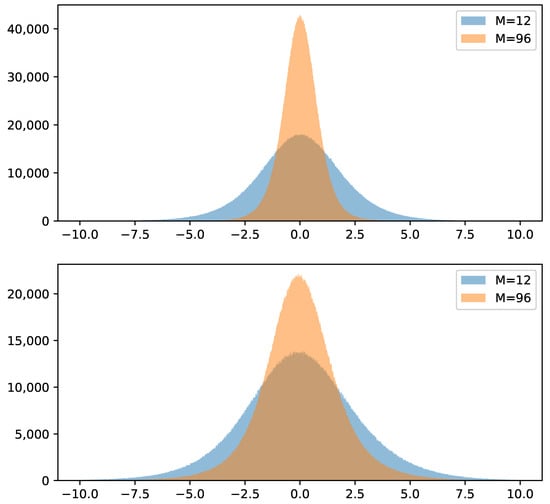
Figure 1 shows histograms of the total hedging errors

$$\widehat{V}+\sum _{m=0}^{{\tau }^{k}M-1}{h}^{{\lambda }_m}\left(y_m^k\right)·\left(p_{m+1}\left(y_{m+1}^k\right)-p_m\left(y_m^k\right)\right)-g({\tau }^k,X_{{\tau }^k}),k=K_H+1,\dots ,K_E,$$

for $d\in \left\{5,10\right\}$ and $M\in \left\{12,96\right\}$.

Figure 1. Total hedging errors for $s_0=100$, $M\in \{12,96\}$, $d=5$ (top) and $d=10$ (bottom) along 4,096,000 sample paths of ${\left(Y_m\right)}_{m=0}^{NM}$. The values of the parameters r, $\delta$, $\sigma$, $\rho$, K, T and N were as in Table 1 and Table 2.

6. Conclusions

In this article, we used deep learning to price and hedge American-style options. In a first step our method employs a neural network version of the Longstaff–Schwartz algorithm to estimate continuation values and derive a candidate optimal stopping rule. The learned stopping rule immediately yields a low-biased estimate of the price. In addition, it can be used to construct an approximate solution of the dual martingale problem of Rogers (2002) and Haugh and Kogan (2004). This gives a high-biased estimate and confidence intervals for the price. To achieve the same pricing accuracy as the more direct approaches of Becker et al. (2019a, 2019b), we had to train the neural network approximations of the continuation values for a longer time. However, computing approximate continuation values has the advantage that they can be used to break the hedging problem into a sequence of subproblems that compute the hedge only from one possible exercise date to the next.

References

- Andersen, Leif. 2000. A simple approach to the pricing of Bermudan swaptions in the multifactor LIBOR market model. The Journal of Computational Finance 3: 5–32. [Google Scholar] [CrossRef]
- Bally, Vlad, Gilles Pagès, and Jacques Printems. 2005. A quantization tree method for pricing and hedging multidimensional American options. Mathematical Finance 15: 119–68. [Google Scholar] [CrossRef]
- Barraquand, Jérôme, and Didier Martineau. 1995. Numerical valuation of high dimensional multivariate American securities. The Journal of Financial and Quantitative Analysis 30: 383–405. [Google Scholar] [CrossRef]
- Becker, Sebastian, Patrick Cheridito, and Arnulf Jentzen. 2019a. Deep optimal stopping. Journal of Machine Learning Research 20: 1–25. [Google Scholar]
- Becker, Sebastian, Patrick Cheridito, Arnulf Jentzen, and Timo Welti. 2019b. Solving high-dimensional optimal stopping problems using deep learning. arXiv arXiv:1908.01602. [Google Scholar]
- Berridge, Steffan J., and Johannes M. Schumacher. 2008. An irregular grid approach for pricing high-dimensional American options. Journal of Computational and Applied Mathematics 222: 94–111. [Google Scholar] [CrossRef]
- Bouchard, Bruno, and Xavier Warin. 2012. Monte-Carlo valuation of American options: Facts and new algorithms to improve existing methods. In Numerical Methods in Finance. Berlin and Heidelberg: Springer, pp. 215–255. [Google Scholar]
- Broadie, Mark, and Menghui Cao. 2008. Improved lower and upper bound algorithms for pricing American options by simulation. Quantitative Finance 8: 845–61. [Google Scholar] [CrossRef]
- Broadie, Mark, and Paul Glasserman. 2004. A stochastic mesh method for pricing high-dimensional American options. Journal of Computational Finance 7: 35–72. [Google Scholar] [CrossRef]
- Bru, Bernard, and Henri Heinich. 1985. Meilleures approximations et médianes conditionnelles. Annales de l’I.H.P. Probabilités et Statistiques 21: 197–224. [Google Scholar]
- Buehler, Hans, Lukas Gonon, Josef Teichmann, and Ben Wood. 2019. Deep hedging. Quantitative Finance 19: 1271–91. [Google Scholar] [CrossRef]
- Carriere, Jacques F. 1996. Valuation of the early-exercise price for options using simulations and nonparametric regression. Insurance: Mathematics and Economics 19: 19–30. [Google Scholar] [CrossRef]
- Chen, Yangang, and Justin W.L. Wan. 2019. Deep neural network framework based on backward stochastic differential equations for pricing and hedging American options in high dimensions. arXiv arXiv:1909.11532. [Google Scholar]
- Egloff, Daniel, Michael Kohler, and Nebojsa Todorovic. 2007. A dynamic look-ahead Monte Carlo algorithm for pricing Bermudan options. Annals of Applied Probability 17: 1138–71. [Google Scholar] [CrossRef]
- Forsyth, Peter A., and Ken R. Vetzal. 2002. Quadratic convergence for valuing American options using a penalty method. SIAM Journal on Scientific Computing 23: 2095–122. [Google Scholar] [CrossRef]
- García, Diego. 2003. Convergence and biases of Monte Carlo estimates of American option prices using a parametric exercise rule. Journal of Economic Dynamics and Control 27: 1855–79. [Google Scholar] [CrossRef]
- Glorot, Xavier, and Yoshua Bengio. 2010. Understanding the difficulty of training deep feedforward neural networks. Paper Presented at Thirteenth International Conference on Artificial Intelligence and Statistics, PMLR, Sardinia, Italy, May 13–15, vol. 9, pp. 249–256. [Google Scholar]
- Han, Jiequn, Arnulf Jentzen, and Weinan E. 2018. Solving high-dimensional partial differential equations using deep learning. Proceedings of the National Academy of Sciences of the United States of America 115: 8505–10. [Google Scholar] [CrossRef]
- Haugh, Martin B., and Leonid Kogan. 2004. Pricing American options: a duality approach. Operations Research 52: 258–70. [Google Scholar] [CrossRef]
- Hull, John C. 2003. Options, Futures and Other Derivatives. London: Pearson. Upper Saddle River: Prentice Hall. [Google Scholar]
- Ioffe, Sergey, and Christian Szegedy. 2015. Batch normalization: accelerating deep network training by reducing internal covariate shift. Paper presented at 32nd International Conference on Machine Learning, ICML 2015, Lille, France, July 6–11, vol. 37, pp. 448–456. [Google Scholar]
- Jain, Shashi, and Cornelis W. Oosterlee. 2015. The stochastic grid bundling method: efficient pricing of Bermudan options and their Greeks. Applied Mathematics and Computation 269: 412–31. [Google Scholar] [CrossRef]
- Kingma, Diederik P., and Jimmy Ba. 2015. Adam: A method for stochastic optimization. Paper Presented at International Conference on Learning Representations, San Diego, CA, USA, May 7–9. [Google Scholar]
- Kohler, Michael, Adam Krzyżak, and Nebojsa Todorovic. 2010. Pricing of high-dimensional American options by neural networks. Mathematical Finance 20: 383–410. [Google Scholar] [CrossRef]
- Kolodko, Anastasia, and John Schoenmakers. 2006. Iterative construction of the optimal Bermudan stopping time. Finance and Stochastics 10: 27–49. [Google Scholar] [CrossRef]
- Lapeyre, Bernard, and Jérôme Lelong. 2019. Neural network regression for Bermudan option pricing. arXiv arXiv:1907.06474. [Google Scholar]
- Longstaff, Francis A., and Eduardo S. Schwartz. 2001. Valuing American options by simulation: a simple least-squares approach. The Review of Financial Studies 14: 113–47. [Google Scholar] [CrossRef]
- Reisinger, Christoph, and Jan H. Witte. 2012. On the use of policy iteration as an easy way of pricing American options. SIAM J. Financial Math. 3: 459–78. [Google Scholar] [CrossRef]
- Rogers, Chris. 2002. Monte Carlo valuation of American options. Mathematical Finance 12: 271–86. [Google Scholar] [CrossRef]
- Rogers, Chris. 2010. Dual valuation and hedging of Bermudan options. SIAM Journal on Financial Mathematics 1: 604–8. [Google Scholar] [CrossRef]
- Sirignano, Justin, and Konstantinos Spiliopoulos. 2018. DGM: A deep learning algorithm for solving partial differential equations. Journal of Computational Physics 375: 1339–64. [Google Scholar] [CrossRef]
- Tilley, James A. 1993. Valuing American options in a path simulation model. Transactions of the Society of Actuaries 45: 83–104. [Google Scholar]
- Tsitsiklis, John N., and Benjamin Van Roy. 2001. Regression methods for pricing complex American-style options. IEEE Transactions on Neural Networks 12: 694–703. [Google Scholar] [CrossRef]