The Distribution of Cross Sectional Momentum Returns When Underlying Asset Returns Are Student’s t Distributed

Abstract

In Kwon and Satchell (2018), a theoretical framework was introduced to investigate the distributional properties of the cross-sectional momentum returns under the assumption that the vector of asset returns over the ranking and holding periods were multivariate normal. In this paper, the framework is extended to derive the corresponding results when the asset returns are multivariate Student’s t. In particular, we derive the probability density function and the moments of the cross-sectional momentum returns and examine in detail the special case of two underlying assets to demonstrate that many of the salient features reported in the empirical literature are consistent with the theoretical implications.

1. Introduction

Empirical investigation of the observed patterns in asset returns has been an active area of research in finance, with momentum, or persistence, in asset returns being one of the more popular examples of this line of research. Of these, perhaps the most prominent is cross-sectional momentum (CSM), which refers to the observation that the set of assets that outperform relative to another set over a prior period tend to continue to outperform over a subsequent period. The existence of CSM is usually tested empirically by sorting the assets according to their returns over a prior “ranking” period, and constructing a portfolio over a subsequent “holding” period by taking a long position in the “winners” and a short position in the “losers”. Statistically significant excess returns from following such a strategy would then support the existence of cross-sectional momentum.

Cross sectional momentum strategies are popular with practitioners since they tend to generate positive returns, while they are popular with academics due to the fact their existence would run contrary to an implication of the efficient market hypothesis that there does not exist any discernible patterns in asset returns. There is an extensive academic literature investigating the properties of CSM returns covering various asset classes, markets, and jurisdictions. The most notable findings are that CSM returns are generally slightly positive, but become highly negative during times of market uncertainty, and that losses during such periods tend to cancel out, or at least significantly reduce, the prior gains.

Various authors, including Fama and French (1992), Jegadeesh and Titman (1993, 2001), Asness (1994), and Israel and Moskowitz (2013), found that momentum strategies are profitable in US equities markets over different time periods dating back to 1927. Analogous results were found for country equity indices by Richards (1997), Asness et al. (1997), Chan et al. (2000), and Hameed and Yuanto (2002), for emerging markets by Rouwenhorst (1998), for exchange rate markets in Okunev and White (2003) and Menkhoff et al. (2012), for commodities by Erb and Harvey (2006), for futures contracts in Moskowitz et al. (2012), and in industries by Sefton and Scowcroft (2004). Similar results were also found by Asness et al. (2013) and Daniel and Moskowitz (2016) for markets in the European Union, Japan, the United Kingdom, and the United States, and across asset classes including fixed income, commodities, foreign exchange, and equity from 1972 through 2013.

Despite the extensive literature on the empirical properties of momentum based returns, there are relatively few that consider the distributional properties of these returns from a theoretical viewpoint, with Kwon and Satchell (2018) being a notable exception that addresses the CSM returns as defined in this paper. Most of the known theoretical results, obtained for example by Lo and MacKinlay (1990), Jegadeesh and Titman (1993), Lewellen (2002), and Moskowitz et al. (2012), are concerned only with the expected values and first order autocorrelations of returns from the so-called weighted relative strength strategy in which the portfolio over the holding period is constructed from all underlying assets weighted, essentially, in proportion to their absolute or relative returns over the ranking period. The reason why we wish to calculate the distribution of CSM returns is that we can then calculate percentiles, quantiles, and related quantities. We can deduce the degree to which moments of returns exist and their precise form. Such information can be used, for example, to assess the fatness of the tails of the distribution and this is valuable for risk management calculations as well as understanding the benefits and limitations of portfolio construction.

By assuming that underlying asset returns are Gaussian, the distribution and the moments of the CSM returns were derived in Kwon and Satchell (2018). In this paper, we extend their results to the case where the underlying asset returns are Student’s t to derive the probability density function and the moments of the CSM returns. The t distribution arises naturally, for example, in a framework where asset volatility is stochastic, and conventional mean-variance analysis will create returns which are very similar to t-distributed returns. The important distinction between Student’s t returns and normal returns is that the distribution of Student’s t has an additional parameter which governs the fatness of the tails of the distribution and can be used to assess tail risk. There is a trade-off between realism and complexity; we would like to use a more complex distribution such as the skewed Student’s t considered in Theodossiou (1998) and Hansen et al. (2010), but the analytical complexity that results becomes prohibitive.

Although the individual asset returns do not exhibit skewness under the generalization to Student’s t, they can be leptokurtic which is a well-established feature in the empirical literature. Moreover, the CSM returns can, and do, exhibit skewness that depends on the statistical properties of the underlying assets. A detailed analysis of the special case of two underlying assets reveals that many of the salient features of the CSM returns reported in the empirical literature are consistent with the theoretical implications from this framework. This analysis is of interest because Kwon and Satchell (2018) were able to show that non-normality was a consequence of the momentum structure, even when the underlying returns were normal. We therefore wish to assess what the impact of assuming non-normality in the underlying returns will have on CSM returns. For example, will it exacerbate non-normality or make very little difference? Answers to this question will shed light on applying CSM to universes of assets which are fundamentally non-normal, such as emerging markets.

It should be pointed out that since we work under the assumption that asset returns over the ranking and holding periods are jointly t-distributed, there are limitations in the properties of momentum returns that can be addressed in the theoretical framework of this paper. For example, it is not possible to adequately address properties that depend on certain firm specific, economic, or financial factors such as liquidity, credit spread, market sentiment, business cycle, and information asymmetry since these factors cannot easily be captured in the distributional assumption on asset returns. Theoretical investigation of such properties would require an extension with the ability to incorporate such factors.

Finally, it may be asked what the connection is between our analysis and the extensive linear factor modelling that dominates the asset pricing literature. This literature essentially says that the time t mean of an asset, say the first, is a linear function of factor returns. In the framework of this paper, we can accommodate such modelling by interpreting the asset mean to be conditional on factor returns.

The remainder of this paper is organized as follows: Section 2 introduces the notation and the key results on multivariate normal distributions, and Section 3 provides a mathematically precise definition of CSM returns. Although the expressions for the CSM return density and the associated moments are quite complex in general, they simplify considerably in the case of two assets with one winner and one loser, and this special case is examined in detail in Section 4, along with implications to the empirically observed features reported in the literature, and the paper concludes with Section 5.

2. Notation and Preliminaries

For the convenience of the reader, we introduce in this section the notation that will be used throughout the paper, and present some known results that will be relied upon in subsequent sections.

2.1. Notation

For any $\mathit{x}\in {\mathbb{R}}^n$, we will write $x_i$ for the i-th coordinate of $\mathit{x}$, and given $\mathit{y}\in {\mathbb{R}}^n$ write $\mathit{x}\prec \mathit{y}$ if and only if $x_i<y_i$ for all $1\le i\le n$. Similarly, given a matrix $M\in {\mathbb{R}}^{m\times k}$, we will write $M_{i,j}$ for the $(i,j)$-th entry of M, and the transpose of a vector or a matrix will be denoted by the superscript ${}^{\prime }$. The vector in ${\mathbb{R}}^n$ with all entries equal to 1 will be denoted ${\mathbf{1}}_n$, and given a subset $A\in {\mathbb{R}}^n$, we will denote by ${\mathbb{I}}_A$ the indicator function on A.

Given a random vector, $\mathit{X}$, with values in a region ${\mathcal{D}}_{\mathit{X}}\subset {\mathbb{R}}^n$, we will write $f_{\mathit{X}}\left(\mathit{x}\right)$ and $F_{\mathit{X}}\left(\mathit{x}\right)$ for the probability density and the cumulative density functions of $\mathit{X}$, respectively. Moreover, given another random vector $\mathit{Y}$, with values in ${\mathcal{D}}_{\mathit{Y}}\subset {\mathbb{R}}^m$, we will denote by $f_{\mathit{X}|\mathit{Y}}\left(\mathit{x}\right|\mathit{y})$ and $F_{\mathit{X}|\mathit{Y}}\left(\mathit{x}\right|\mathit{y})$ the conditional probability density and conditional cumulative density functions of $\mathit{X}$ given $\mathit{Y}=\mathit{y}$, respectively.

For any $n\in \mathbb{N}$, let $\left[n\right]=\{1,2,\dots ,n\}$ and let $S_n$ be the set of permutations of $\left[n\right]$. We will denote the permutation that maps $1\mapsto i_1,2\mapsto i_2,\dots ,n\mapsto i_n$ by a sequence $(i_1,i_2,\dots ,i_n)$, and given any $\tau \in S_n$ write $\tau \left(i\right)$ for the image of i under $\tau$ so that if $\tau =(1,3,2)$, for example, then $\tau \left(1\right)=1$, $\tau \left(2\right)=3$, and $\tau \left(3\right)=2$. Given a permutation $\tau \in S_n$, we will denote by $P_{\tau }\in {\mathbb{R}}^{n\times n}$ the permutation matrix corresponding to $\tau$ and denote by $D_n\in {\mathbb{R}}^{(n-1)\times n}$ the matrix

$$\begin{array}{c}\hfill D_n=\left[\begin{array}{c}-1\hspace{1em}\hspace{1em}1\hspace{1em}\hspace{1em}0\hspace{1em}\hspace{1em}0\hspace{1em}\hspace{1em}\cdots \hspace{1em}\hspace{1em}0\hspace{1em}\hspace{1em}0\hspace{1em}\hspace{1em}0\\ 0\hspace{1em}\hspace{1em}-1\hspace{1em}\hspace{1em}1\hspace{1em}\hspace{1em}0\hspace{1em}\hspace{1em}\cdots \hspace{1em}\hspace{1em}0\hspace{1em}\hspace{1em}0\hspace{1em}\hspace{1em}0\\ \hspace{1em}\hspace{1em}\hspace{1em}\hspace{1em}\cdots \cdots \cdots \cdots \cdots \cdots \hspace{1em}\hspace{1em}\hspace{1em}\hspace{1em}\\ 0\hspace{1em}\hspace{1em}\hspace{1em}0\hspace{1em}\hspace{1em}0\hspace{1em}\hspace{1em}0\hspace{1em}\hspace{1em}\cdots \hspace{1em}\hspace{1em}0\hspace{1em}\hspace{1em}-1\hspace{1em}\hspace{1em}1\end{array}\right].\end{array}$$

(1)

The elements of the permutation group $S_n$ act naturally on the set of polynomials, $\mathbb{R}[x_1,\dots ,x_n]$ by the rule

$$\begin{array}{c}\hfill \tau p(x_1,\dots ,x_n)=p(x_{{\tau }_1},\dots ,x_{{\tau }_n})\end{array}$$

for any polynomial $p\in \mathbb{R}[x_1,\dots ,x_n]$ and $\tau \in S_n$. For any $n_1,n_2\in \mathbb{N}$, let $p_{n_1,2n_2}\in \mathbb{R}[x_1,\dots ,x_{n_1+2n_2}]$ be the polynomial

$$\begin{array}{c}\hfill p_{n_1,2n_2}(x_1,\dots ,x_{n_1+2n_2})=\left(\prod _{i=1}^{n_1}{x}_i\right)\left(\prod _{i=1}^{n_2}{(x_{n_1+2i}-x_{n_1+2i-1})}^2\right).\end{array}$$

(2)

Denote by $Z(n_1,2n_2)$ the stabilizer of $p_{n_1,2n_2}$ under the action of $S_{n_1+2n_2}$ so that

$$\begin{array}{c}\hfill Z(n_1,2n_2)=\{\tau \in S_{n_1+2n_2}\mid \tau p_{n_1,2n_2}=p_{n_1,2n_2}\},\end{array}$$

(3)

and let $Q(n_1,2n_2)=S_{n_1+2n_2}/Z(n_1,2n_2)$ be the quotient group,1 with elements of $Q(n_1,2n_2)$ identified with their coset representatives $\tau \in S_{n_1+2n_2}$. Finally, define

$$\begin{array}{c}\hfill {\left[n\right]}^m=\prod _{i=1}^m\{1,2,\dots ,n\}=\{(i_1,i_2,\dots ,i_m)\mid 1\le i_j\le n,1\le j\le m\}\end{array}$$

(4)

as the m-fold Cartesian product of $\left[n\right]=\{1,2,\dots ,n\}$.

2.2. Multivariate Normal Distributions

The density of an n-dimensional normal distribution with mean $\mathit{\mu }$ and covariance $\mathsf{\Sigma }$ at $\mathit{x}\in {\mathbb{R}}^n$ will be denoted ${\varphi }_n(\mathit{x};\mathit{\mu },\mathsf{\Sigma })$, and the corresponding cumulative density function will be denoted ${\mathsf{\Phi }}_n(\mathit{x};\mathit{\mu },\mathsf{\Sigma })$. In general, given random variables ${\mathit{X}}_1,\dots ,{\mathit{X}}_n$, their joint probability density function will be denoted $f_{{\mathit{X}}_1,\cdots ,{\mathit{X}}_n}$, and we will write $F_{{\mathit{X}}_1,\cdots ,{\mathit{X}}_n}$ for the cumulative density function.

Theorem 1.

Let $n_1,n_2\in \mathbb{N}$ and suppose $\mathit{X}\sim {\mathcal{N}}_{n_1+n_2}\left(\mathit{\mu },\mathsf{\Sigma }\right)$, where

$$\begin{array}{c}\hfill \mathit{X}=\left[\begin{array}{c}{\mathit{X}}_1\\ {\mathit{X}}_2\end{array}\right],\mathit{\mu }=\left[\begin{array}{c}{\mathit{\mu }}_1\\ {\mathit{\mu }}_2\end{array}\right],\mathsf{\Sigma }=\left[\begin{array}{cc}{\mathsf{\Sigma }}_{1,1}& {\mathsf{\Sigma }}_{1,2}\\ {\mathsf{\Sigma }}_{2,1}& {\mathsf{\Sigma }}_{2,2}\end{array}\right],\end{array}$$

(5)

with ${\mathit{X}}_i,{\mathit{\mu }}_i\in {\mathbb{R}}^{n_i}$ and ${\mathsf{\Sigma }}_{i,j}\in {\mathbb{R}}^{n_i\times n_j}$ for $1\le i,j\le 2$, and Σ positive definite. Then, the conditional distribution of ${\mathit{X}}_1$ given ${\mathit{X}}_2$ is normal with mean and covariance

$$\begin{array}{cc}\hfill {\mathit{\mu }}_{{\mathit{X}}_1\mid {\mathit{X}}_2}& ={\mathit{\mu }}_1+{\mathsf{\Sigma }}_{1,2}{\mathsf{\Sigma }}_{2,2}^{-1}({\mathit{X}}_2-{\mathit{\mu }}_2),\hfill \end{array}$$

(6)

$$\begin{array}{cc}\hfill {\mathsf{\Sigma }}_{{\mathit{X}}_1\mid {\mathit{X}}_2}& ={\mathsf{\Sigma }}_{1,1}-{\mathsf{\Sigma }}_{1,2}{\mathsf{\Sigma }}_{2,2}^{-1}{\mathsf{\Sigma }}_{2,1},\hfill \end{array}$$

(7)

respectively, and ${\varphi }_{n_1+n_2}(\mathit{x};\mathit{\mu },\mathsf{\Sigma })$ decomposes as

$$\begin{array}{c}\hfill {\varphi }_{n_1+n_2}(\mathit{x};\mathit{\mu },\mathsf{\Sigma })={\varphi }_{n_1}\left({\mathit{x}}_1;{\mathit{\mu }}_{{\mathit{X}}_1\mid {\mathit{X}}_2},{\mathsf{\Sigma }}_{{\mathit{X}}_1\mid {\mathit{X}}_2}\right){\varphi }_{n_2}({\mathit{x}}_2;{\mathit{\mu }}_2,{\mathsf{\Sigma }}_{2,2}).\end{array}$$

(8)

Proof. 

Refer to Muirhead (1982) Theorem 1.2.11.  □

Given an n-dimensional random vector $\mathit{X}$ and $\mathit{p}=(p_1,\dots ,p_m)\in {\{1,2,\dots ,n\}}^m$, we will denote by ${\mathit{\mu }}_{\mathit{p}}\left(\mathit{X}\right)$ the $\mathit{p}$-th moment of $\mathit{X}$ so that

$$\begin{array}{c}\hfill {\mathit{\mu }}_{\mathit{p}}\left(\mathit{X}\right)=\mathbb{E}\left[\prod _{i=1}^m{X}_{p_i}\right].\end{array}$$

(9)

Note that the subscripts, $p_i$, in (9) may be repeated so that the above definition is equivalent to the more familiar definition of moments in which the powers of the components of $\mathit{X}$ appear inside the expectation on the right-hand side, viz. $\mathbb{E}\left[{\prod }_{i=1}^n{X}_i^{k_i}\right]$ with $0\le k_i\in \mathbb{N}$ for $1\le i\le n$. For example, we have $\mathbb{E}\left[X_1^2{X}_2^3\right]=\mathbb{E}\left[X_1{X}_1{X}_2{X}_2{X}_2\right]$, and so in the notation of (9) we have $m=5$, $\mathit{d}=(d_1,d_2,d_3,d_4,d_5)=(1,1,2,2,2)$, and ${\mu }_{(1,1,2,2,2)}\left(\mathit{X}\right)=\mathbb{E}\left[X_1^2{X}_2^3\right]$.

Theorem 2.

Let $\mathit{X}\sim {\mathcal{N}}_n(\mathit{\mu },\mathsf{\Sigma })$, where $n\in \mathbb{N}$, $\mathit{\mu }\in {\mathbb{R}}^n$ and $\mathsf{\Sigma }\in {\mathbb{R}}^{n\times n}$ is positive definite. Then, for any $\mathit{p}=(p_1,\dots ,p_m)\in {\{1,2,\dots ,n\}}^m$, we have

$$\begin{array}{c}\hfill {\mu }_{\mathit{p}}\left(\mathit{X}\right)=\sum _{\begin{array}{c}k,l\in \mathbb{N}\\ k+2l=m\end{array}}\sum _{\tau \in Q(k,2l)}\left(\prod _{i=1}^k{\mu }_{p_{{\tau }_i}}\right)\left(\prod _{i=1}^l{\mathsf{\Sigma }}_{p_{{\tau }_{k+2i-1}},p_{{\tau }_{k+2i}}}\right).\end{array}$$

(10)

In particular, if $\mathit{\mu }=\mathbf{0}$ and m is even, then

$$\begin{array}{c}\hfill {\mu }_{\mathit{p}}\left(\mathit{X}\right)=\sum _{\tau \in Q(0,m)}\prod _{i=1}^{\frac{1}{2}m}{\mathsf{\Sigma }}_{p_{{\tau }_{2i-1}},p_{{\tau }_{2i}}}.\end{array}$$

(11)

Proof. 

Refer to Withers (1985) Theorem 1.1.  □

An alternative expression for ${\mu }_{\mathit{p}}\left(\mathit{X}\right)$, where $\mathit{X}$ is multivarite normal, is given in Kan (2008) Proposition 2.

Corollary 1.

Let $X\sim {\mathcal{N}}_1(\mu ,{\sigma }^2)$. Then, for any $m\in \mathbb{N}$, the m-th moment of X is given by

$$\begin{array}{c}\hfill {\mu }_m\left(X\right)=\sum _{\begin{array}{c}i=0\\ i\mathit{even}\end{array}}^m\left(\genfrac{}{}{0pt}{}{m}{i}\right)(i-1)!!{\sigma }^i{\mu }^{m-i},\end{array}$$

(12)

where $k!!={\prod }_{i=0}^{\lfloor \frac{k}{2}\rfloor }(k-2i)$ is the double factorial of $k\in \mathbb{N}$. In the special case where $\mu =0$ and m is even, we have ${\mu }_m\left(X\right)=(m-1)!!{\sigma }^m$.

Proof. 

Follows from Theorem 2, since the inner sum in (10), for which $2l=i$, consists of $\left(\genfrac{}{}{0pt}{}{m}{i}\right)(i-1)!!$ identical terms that are all equal to ${\sigma }^i{\mu }^{m-i}$.  □

2.3. Multivariate Student’s t Distribution

Asset returns are often assumed to be normally distributed in the academic literature for theoretical convenience, in which case they are completely determined by the location and the scale parameters. However, it is widely reported in the empirical literature that the observed asset returns exhibit excess kurtosis. Student’s t-distribution is a distribution from the elliptical family with an additional parameter $\nu$, viz. number of degrees of freedom that controls the kurtosis. The Student’s t distribution reduces to the normal in the limit as $\nu \to \infty$, and hence provides a convenient framework under which to investigate the impact of excess kurtosis in the underlying asset returns on the distributional properties of the CSM return. This subsection provides a brief summary of the key properties of the Student’s t distribution that will be required in the remainder of this paper.

The t distribution has a long history in mathematical statistics. The univariate probability density function (pdf), t ($\mu$,${\sigma }^2$,$\nu$), of a t-variate with mean $\mu$, scale parameter $\sigma$, and degrees of freedom $\nu$ is given by

$$\begin{array}{c}\hfill t(\mu ,{\sigma }^2,\nu )=\frac{\mathsf{\Gamma }\left(\frac{\nu +1}{2}\right)}{\sigma \sqrt{\nu \pi }\mathsf{\Gamma }\left(\frac{\nu }{2}\right)}{\left(1+\frac{1}{\nu }{\left(\frac{x-\mu }{\sigma }\right)}^2\right)}^{-\frac{1}{2}(\nu +1)}.\end{array}$$

(13)

From the origins of the t-test in mathematical finance, it is clear that we can write the corresponding random variable as $x=\mu +z/Y$, where z and Y are independent, $z\sim \mathcal{N}(0,{\sigma }^2)$, $Y=\sqrt{g/\nu }$, and $g\sim {\chi }^2\left(\nu \right)$.

In extending the definition of the t distribution to the multivariate case, we are faced with a choice. Although the choice $\mathit{z}\sim {\mathcal{N}}_n\left(\mathbf{0},\mathsf{\Sigma }\right)$ is clear, Y can be defined in various ways. For example:

• each component, $z_i$, of $\mathit{z}$ is normalized by independent $Y_i=\sqrt{g_i/{\nu }_i}$ with same or differing ${\nu }_i$,
• $Y_i$ could be jointly dependent,
• single common Y.

All three of these choices have a stochastic volatility interpretation corresponding to

• idiosyncratic shocks,
• common factor shocks,
• economy-wide or market-wide shock.

Although we have chosen the final characterization, cross sectional momentum could also be analyzed under other characterizations.

Throughout this paper, the probability density function of n-dimensional Student’s t distribution, ${St}_{n_1+n_2}\left(\mathit{\mu },\mathsf{\Sigma },\nu \right)$, with $\nu$ degrees of freedom, location $\mathit{\mu }$, and shape matrix $\mathsf{\Sigma }$ at $\mathit{x}\in {\mathbb{R}}^n$ will be denoted $t_n(\mathit{x};\mathit{\mu },\mathsf{\Sigma },\nu )$, and we will write $T_n(\mathit{x};\mathit{\mu },\mathsf{\Sigma },\nu )$ for the corresponding cumulative density function. The next theorem shows that multivariate Student’s t distribution is closed under conditioning, in the sense that the conditional density of a subset given its complement is again Student’s t. This property will be crucial in the investigation of the CSM returns in later sections.

Theorem 3.

Let $n_1,n_2\in \mathbb{N}$ and suppose $\mathit{X}\sim {St}_{n_1+n_2}\left(\mathit{\mu },\mathsf{\Sigma },\nu \right)$, where $\nu \in {\mathbb{R}}_{+}$,

$$\begin{array}{c}\hfill \mathit{X}=\left[\begin{array}{c}{\mathit{X}}_1\\ {\mathit{X}}_2\end{array}\right],\mathit{\mu }=\left[\begin{array}{c}{\mathit{\mu }}_1\\ {\mathit{\mu }}_2\end{array}\right],\mathsf{\Sigma }=\left[\begin{array}{cc}{\mathsf{\Sigma }}_{1,1}& {\mathsf{\Sigma }}_{1,2}\\ {\mathsf{\Sigma }}_{2,1}& {\mathsf{\Sigma }}_{2,2}\end{array}\right],\end{array}$$

(14)

with ${\mathit{X}}_i,{\mathit{\mu }}_i\in {\mathbb{R}}^{n_i}$ and ${\mathsf{\Sigma }}_{i,j}\in {\mathbb{R}}^{n_i\times n_j}$ for $1\le i,j\le 2$, and Σ positive definite. Then, the conditional distribution of ${\mathit{X}}_1$ given ${\mathit{X}}_2$ is Student’s t with degrees of freedom ${\nu }_{{\mathit{X}}_1\mid {\mathit{X}}_2}=\nu +n_2$, and location and shape matrix

$$\begin{array}{cc}\hfill {\mathit{\mu }}_{{\mathit{X}}_1\mid {\mathit{X}}_2}& ={\mathit{\mu }}_1+{\mathsf{\Sigma }}_{1,2}{\mathsf{\Sigma }}_{2,2}^{-1}({\mathit{X}}_2-{\mathit{\mu }}_2),\hfill \end{array}$$

(15)

$$\begin{array}{cc}\hfill {\mathsf{\Sigma }}_{{\mathit{X}}_1\mid {\mathit{X}}_2}& =\frac{\nu +{\left({\mathit{X}}_2-{\mathit{\mu }}_2\right)}^{\prime }{\mathsf{\Sigma }}_{2,2}^{-1}\left({\mathit{X}}_2-{\mathit{\mu }}_2\right)}{\nu +n_2}\left({\mathsf{\Sigma }}_{1,1}-{\mathsf{\Sigma }}_{1,2}{\mathsf{\Sigma }}_{2,2}^{-1},{\mathsf{\Sigma }}_{2,1}\right),\hfill \end{array}$$

(16)

respectively, and $t_{n_1+n_2}(\mathit{x};\mathit{\mu },\mathsf{\Sigma },\nu )$ decomposes as

$$\begin{array}{c}\hfill t_{n_1+n_2}(\mathit{x};\mathit{\mu },\mathsf{\Sigma },\nu )=t_{n_1}\left({\mathit{x}}_1;{\mathit{\mu }}_{{\mathit{X}}_1\mid {\mathit{X}}_2},{\mathsf{\Sigma }}_{{\mathit{X}}_1\mid {\mathit{X}}_2},{\nu }_{{\mathit{X}}_1\mid {\mathit{X}}_2}\right)t_{n_2}({\mathit{x}}_2;{\mathit{\mu }}_2,{\mathsf{\Sigma }}_{2,2},\nu ).\end{array}$$

(17)

Proof. 

Refer to Roth (2013) Appendix A.6, or Muirhead (1982) Problems 1.29 and 1.30.  □

Although a Student’s t distribution does not have finite moments of all orders, the next theorem provides an explicit expression for those that do exist.

Theorem 4.

Let $\mathit{X}\sim {St}_n(\mathit{\mu },\mathsf{\Sigma },\nu )$, where $n\in \mathbb{N}$, $\nu \in {\mathbb{R}}_{+}$, $\mathit{\mu }\in {\mathbb{R}}^n$ and $\mathsf{\Sigma }\in {\mathbb{R}}^{n\times n}$ is positive definite. Moreover, for any $m\in \mathbb{N}$, denote by ${\mathcal{P}}_m$ the set of subsets of the set $\{1,2,\dots ,m\}$ of size k such that $m-k$ is even, where $0\le k\le m$. Then, for any $\mathit{p}=(p_1,\dots ,p_m)\in {\{1,2,\dots ,n\}}^m$ such that $m<\nu$, we have

$$\begin{array}{cc}\hfill {\mu }_{\mathit{p}}\left(\mathit{X}\right)& =\sum _{P\in {\mathcal{P}}_m}\frac{\mathsf{\Gamma }\left(\frac{\nu }{2}-\frac{1}{2}\left|P^c\right|\right)}{\mathsf{\Gamma }\left(\frac{\nu }{2}\right)}{\left(\frac{\nu }{2}\right)}^{\frac{1}{2}\left|P^c\right|}\prod _{k\in P}{\mu }_{p_{i_k}}\sum _{\tau \in Q(0,|P^c\left|\right)}\left(\prod _{j=1}^{\frac{1}{2}\left|P^c\right|}{\mathsf{\Sigma }}_{p_{i_{{\tau }_{2j-1}}},p_{i_{{\tau }_{2j}}}}\right),\hfill \end{array}$$

(18)

where $P^c=\{i_1,i_2,\dots ,i_{k+2l}\}$ in the final sum.

Proof. 

Refer to Appendix A.  □

Setting $n=1$ gives the moments of the one-dimensional Student’s t distribution.

Corollary 2.

Let $X\sim {St}_1(\mu ,{\sigma }^2,\nu )$. Then, for any $m\in \mathbb{N}$ such that $m<\nu$, the m-th moment of X is given by

$$\begin{array}{c}\hfill {\mu }_m\left(X\right)=\sum _{\begin{array}{c}k=0\\ k\mathrm{even}\end{array}}^m\left(\genfrac{}{}{0pt}{}{m}{k}\right)(k-1)!!\frac{\mathsf{\Gamma }\left(\frac{1}{2}(\nu -k)\right)}{\mathsf{\Gamma }\left(\frac{\nu }{2}\right)}{\left(\frac{\nu }{2}\right)}^{\frac{k}{2}}{\mu }^{m-k}{\sigma }^k,\end{array}$$

(19)

where $k!!$ is the double factorial defined in Corollary 1.

Proof. 

Follows from similar arguments to Theorem 4 noting that the indices $p_{i_j}$ are all equal in this case.  □

For an alternative derivation of the moments of Student’s t distribution, refer to Kirkby et al. (2019).

2.4. Unified Skew t Family of Distributions

Multivariate skew-normal (SN) distributions were introduced in Azzalini and Valle (1985) to generalize normal distributions to those that allow non-zero skewness, and the seemingly disparate distributions related to the multivariate SN distributions were brought together under the umbrella of the so-called unified skew-normal (SUN) family of distributions in Arellano-Valle and Azzalini (2006), where it was shown that the SUN family contains many of these skew-normal variants as special cases. The extension of the normal family to those with non-zero skewness was then extended to the elliptical family of distributions in Arellano-Valle and Genton (2010). In what follows, we only summarize the results on the extension for the multivariate Student’s t distributions that will be required in this paper, and refer the reader to Arellano-Valle and Genton (2010) and Jamalizadeh and Balakrishnan (2012) for the details.

Given $\nu \in {\mathbb{R}}_{+}$, $n_i\in \mathbb{N}$, ${\mathit{\mu }}_i\in {\mathbb{R}}^{n_i}$, ${\mathsf{\Sigma }}_{i,j}\in {\mathbb{R}}^{n_1\times n_2}$ for $1\le i\le j$, where ${\mathsf{\Sigma }}_{2,1}^{\prime }={\mathsf{\Sigma }}_{1,2}$ and ${\mathsf{\Sigma }}_{i,i}$ are positive definite, let

$$\begin{array}{c}\hfill \left[\begin{array}{c}{\mathit{X}}_1\\ {\mathit{X}}_2\end{array}\right]\sim {St}_{n_1+n_2}\left(\left[\begin{array}{c}{\mathit{\mu }}_1\\ {\mathit{\mu }}_2\end{array}\right],\left[\begin{array}{cc}{\mathsf{\Sigma }}_{1,1}& {\mathsf{\Sigma }}_{1,2}\\ {\mathsf{\Sigma }}_{1,2}^{\prime }& {\mathsf{\Sigma }}_{2,2}\end{array}\right],\nu \right).\end{array}$$

(20)

Then, the probability density function, $f_{\mathit{U}}\left(\mathit{u}\right)$, of an $n_1$-dimensional unified skew t (SUT) distributed random variable, $\mathit{U}$, associated with ${({\mathit{X}}_1^{\prime },{\mathit{X}}_2^{\prime })}^{\prime }$ given by

$$\begin{array}{c}\hfill f_{\mathit{U}}\left(\mathit{u}\right)=\frac{t_{n_2}(\mathit{u};{\mathit{\mu }}_2,{\mathsf{\Sigma }}_{2,2},\nu )}{T_{n_1}\left(\mathbf{0};-{\mathit{\mu }}_1,{\mathsf{\Sigma }}_{1,1},\nu \right)}{T}_{n_1}\left(\mathbf{0};-{\mathit{\mu }}_1-{\mathsf{\Sigma }}_{1,2}{\mathsf{\Sigma }}_{2,2}^{-1}(\mathit{u}-{\mathit{\mu }}_2),{\mathsf{\Sigma }}_{1,1;2}\left(\mathit{u}\right),\nu +n_2\right),\end{array}$$

(21)

where

$$\begin{array}{c}\hfill {\mathsf{\Sigma }}_{1,1;2}\left(\mathit{u}\right)=\frac{\nu +{\left(\mathit{u}-{\mathit{\mu }}_2\right)}^{\prime }{\mathsf{\Sigma }}_{2,2}^{-1}\left(\mathit{u}-{\mathit{\mu }}_2\right)}{\nu +n_2}\left({\mathsf{\Sigma }}_{1,1}-{\mathsf{\Sigma }}_{1,2}{\mathsf{\Sigma }}_{2,2}^{-1}{\mathsf{\Sigma }}_{2,1}\right).\end{array}$$

(22)

The key characteristic of $f_{\mathit{U}}\left(\mathit{u}\right)$ is that it is a product of an $n_2$-dimensional Student’s t density and an $n_1$-dimensional cumulative Student’s t density with the variable $\mathit{u}$ appearing as the main variable in the former and in the mean and variance parameters of the latter. As will be seen, the densities of cross sectional momentum returns will be a weighted sum of these SUT distributions.

3. Cross-Sectional Momentum Returns with Student’s $\mathit{t}$ Distributed Asset Returns

In this section, we derive the distributional properties of the cross sectional momentum (CSM) returns under the assumption that the underlying asset returns are multivariate Student’s t. We begin by recalling the mathematically precise definition of the CSM return from Kwon and Satchell (2018).

Let $0<m_{+},m_{-},n\in \mathbb{N}$ such that $m_{+}+m_{-}\le n$, and for each $1\le i\le n$ denote by $r_{i,t}$ the return on asset i at time t. Moreover, let

$$\begin{array}{cc}\hfill {\mathit{r}}_t& ={(r_{1,t},\dots ,r_{n,t})}^{\prime }\in {\mathbb{R}}^n,\hfill \end{array}$$

(23)

and for any $\tau \in S_n$, define

$$\begin{array}{cc}\hfill r_{\tau ,m_{\pm },t}& =\frac{1}{m_{+}}\sum _{i=1}^{m_{+}}{r}_{{\tau }_i,t}-\frac{1}{m_{-}}\sum _{i=1}^{m_{-}}{r}_{{\tau }_{n-m_{-}+i},t}\in \mathbb{R},\hfill \end{array}$$

(24)

$$\begin{array}{cc}\hfill x_{{\tau }_i,t}& =r_{{\tau }_{i+1},t}-r_{{\tau }_i,t}\in \mathbb{R},1\le i\le n-1,\hfill \end{array}$$

(25)

$$\begin{array}{cc}\hfill {\mathit{x}}_{\tau ,t}& ={(x_{{\tau }_1,t},\dots ,x_{{\tau }_{n-1},t})}^{\prime }\in {\mathbb{R}}^{n-1},\hfill \end{array}$$

(26)

$$\begin{array}{cc}\hfill {\mathit{z}}_{\tau ,t}& ={\left(r_{\tau ,m_{\pm },t+1},{\mathit{x}}_{\tau ,t}^{\prime }\right)}^{\prime }\in {\mathbb{R}}^n.\hfill \end{array}$$

(27)

Note that any given $\tau \in S_n$ defines an ordering, $r_{t,{\tau }_1}>r_{t,{\tau }_2}>\cdots >r_{t,{\tau }_n}$, of the components of ${\mathit{r}}_t$. Thus, $r_{\tau ,m_{\pm },t}$ represents the return on a portfolio where the top $m_{+}$ ranked assets are equally weighted and held long while the bottom $m_{-}$ assets are equally weighted and held short. The assumption of equal weighting is for notational simplicity only, and not crucial for the general theoretical results. Note also that ${\mathit{x}}_{\tau ,t}$ is defined to allow the ranking of the components of ${\mathit{r}}_t$ corresponding to $\tau \in S_n$ to be written succinctly as ${\mathit{x}}_{\tau ,t}\prec {\mathbf{0}}_{n-1}$.

Definition 1.

The $(m_{+},m_{-})$-cross sectional momentum return, $r_{m_{\pm },t+1}$, is defined by

$$\begin{array}{c}\hfill r_{m_{\pm },t+1}=\sum _{\tau \in S_n}{\mathbb{I}}_{\{{\mathit{x}}_{\tau ,t}\prec {\mathbf{0}}_{n-1}\}}{r}_{\tau ,m_{\pm },t+1},\end{array}$$

(28)

where ${\mathbb{I}}_A$, for any subset $A\subset {\mathbb{R}}^n$, denotes the indicator function on the set A.

For intuition behind the definition of $r_{m_{\pm },t+1}$, note that the components of ${\mathit{r}}_t$, representing asset returns over the ranking period, can be arranged in any of the $n!$ orderings corresponding to the permutations $\tau \in S_n$. For each such ranking $r_{t,{\tau }_1}>r_{t,{\tau }_2}>\cdots >r_{t,{\tau }_n}$, the $m_{+}$ winner returns over the holding period are $r_{t+1,{\tau }_1},\dots ,r_{t+1,{\tau }_{m_{+}}}$ while the $m_{-}$ loser returns are $r_{t+1,{\tau }_{n-m_{+}1}},\dots ,r_{t+1,{\tau }_n}$. Equally weighting the returns in the winner and the loser portfolios gives $r_{\tau ,m_{\pm },t+1}$, and since the ranking of components of ${\mathit{r}}_t$ determined by $\tau \in S_n$ is equivalent to the condition ${\mathit{x}}_{\tau ,t}\prec {\mathbf{0}}_{n-1}$, summing over all possible $r_{\tau ,m_{\pm },t+1}$ and prefixing by the matching indicator function gives the expression for $r_{m_{\pm },t+1}$ in (28).

For the remainder of this paper, we make the following assumption on the distribution of ${\left({\mathit{r}}_t^{\prime },{\mathit{r}}_{t+1}\right)}^{\prime }$.

Assumption 1.

The vector of returns, ${({\mathit{r}}_t^{\prime },{\mathit{r}}_{t+1}^{\prime })}^{\prime }$, is multivariate Student’s t distributed so that

$$\begin{array}{c}\hfill \left[\begin{array}{c}{\mathit{r}}_{t+1}\\ {\mathit{r}}_t\end{array}\right]\sim {St}_{2n}\left(\left[\begin{array}{c}{\mathit{\mu }}_{t+1}\\ {\mathit{\mu }}_t\end{array}\right],\left[\begin{array}{cc}{\mathsf{\Sigma }}_{t+1,t+1}& {\mathsf{\Sigma }}_{t+1,t}\\ {\mathsf{\Sigma }}_{t,t+1}& {\mathsf{\Sigma }}_{t,t}\end{array}\right],\nu \right),\end{array}$$

(29)

with $\nu \in {\mathbb{R}}_{+}$, ${\mathit{\mu }}_u\in {\mathbb{R}}^n$, and ${\mathsf{\Sigma }}_{u,v}\in {\mathbb{R}}^{n\times n}$, where $u,v\in \{t,t+1\}$.

Since the t-distribution is symmetric, there are limitations on the properties of asset returns that can be captured adequately by the above assumption as already discussed in Section 1. Nevertheless, the assumption is sufficiently general to accommodate linear factor models and econometric models such as vector autoregressive moving average models where the factors and noise terms, respectively, are t-distributed. Moreover, the framework also allows consideration of more general cases where ${\mathit{\mu }}_t$ and ${\mathit{\mu }}_{t+1}$ are conditional means linear in factors without requiring the factors themselves to be multivariate t. However, since the analysis in later sections will show that momentum returns are nonlinear in the underlying asset returns, the common practise of regressing momentum returns on the various factors must be interpreted as a best linear prediction rather than a conditional expectation in such cases. We now derive the probability density function, $f_{m_{\pm },t+1}\left(r\right)$, of the CSM return $r_{m_{\pm },t+1}$.

Theorem 5.

Suppose that ${({\mathit{r}}_t^{\prime },{\mathit{r}}_{t+1}^{\prime })}^{\prime }$ satisfies Assumption 1. Then, the probability density function, $f_{m_{\pm },t+1}\left(r\right)$, of the cross sectional momentum return, $r_{m_{\pm },t+1}$, is given by

$$\begin{array}{c}\hfill f_{m_{\pm },t+1}\left(r\right)=\sum _{\tau \in S_n}{t}_1\left(r;{\mathit{\iota }}^{\prime }{P}_{\tau }{\mathit{\mu }}_{t+1},{\mathit{\iota }}^{\prime }{P}_{\tau }{\mathsf{\Sigma }}_{t+1,t+1}{P}_{\tau }^{\prime }\mathit{\iota },\nu \right)T_{n-1}\left(\mathbf{0};{\lambda }_{\tau }\left(r\right),{\mathsf{\Lambda }}_{\tau }\left(r\right),\nu +1\right),\end{array}$$

(30)

where $\mathit{\iota }={\left({\mathbf{1}}_{m_{+}}^{\prime },{\mathbf{0}}_{n-m_{+}-m_{-}}^{\prime },-{\mathbf{1}}_{n_{-}}^{\prime }\right)}^{\prime }$,

$$\begin{array}{cc}\hfill {\lambda }_{\tau }\left(r\right)& =D_n{P}_{\tau }{\mathit{\mu }}_t+\frac{\left(r-{\mathit{\iota }}^{\prime }{P}_{\tau }{\mathit{\mu }}_{t+1}\right)}{{\mathit{\iota }}^{\prime }{P}_{\tau }{\mathsf{\Sigma }}_{t+1,t+1}{P}_{\tau }^{\prime }{\mathit{\iota }}^{\prime }}D{P}_{\tau }{\mathsf{\Sigma }}_{t,t+1}{P}_{\tau }^{\prime }\mathit{\iota },\hfill \end{array}$$

(31)

$$\begin{array}{c}\hfill \begin{array}{cc}\hfill {\mathsf{\Lambda }}_{\tau }\left(r\right)& =\frac{\nu +{\left({\mathit{\iota }}^{\prime }{P}_{\tau }{\mathsf{\Sigma }}_{t+1,t+1}{P}_{\tau }^{\prime }{\mathit{\iota }}^{\prime }\right)}^{-1}{\left(r-{\mathit{\iota }}^{\prime }{P}_{\tau }{\mathit{\mu }}_{t+1}\right)}^2}{\nu +1}\hfill \\ \hfill & \left(D_n{P}_{\tau }{\mathsf{\Sigma }}_{t,t}{P}_{\tau }^{\prime }{D}_n^{\prime }-\frac{D_n{P}_{\tau }{\mathsf{\Sigma }}_{t,t+1}{P}_{\tau }^{\prime }\mathit{\iota }{\mathit{\iota }}^{\prime }{P}_{\tau }{\mathsf{\Sigma }}_{t+1,t}{P}_{\tau }^{\prime }{D}_n^{\prime }}{{\mathit{\iota }}^{\prime }{P}_{\tau }{\mathsf{\Sigma }}_{t+1,t+1}{P}_{\tau }^{\prime }{\mathit{\iota }}^{\prime }}\right),\hfill \end{array}\end{array}$$

(32)

and we define $T_0\equiv 1$. Alternatively,

$$\begin{array}{c}\hfill \begin{array}{cc}\hfill f_{m_{\pm },t+1}\left(r\right)& =\sum _{\tau \in S_n}{\int }_{{\mathbb{R}}_{-}^{n-1}}{t}_1\left(r;{\gamma }_{\tau }\left(\mathit{x}\right),{\mathsf{{\rm Y}}}_{\tau }\left(\mathit{x}\right),\nu +n-1\right)t_{n-1}\left(\mathit{x};D_n{P}_{\tau }{\mathit{\mu }}_t,D_n{P}_{\tau }{\mathsf{\Sigma }}_{t,t}{P}_{\tau }^{\prime }{D}_n^{\prime },\nu \right)d\mathit{x},\hfill \end{array}\end{array}$$

(33)

where

$$\begin{array}{cc}\hfill {\gamma }_{\tau }\left(\mathit{x}\right)& ={\mathit{\iota }}^{\prime }{P}_{\tau }{\mathit{\mu }}_{t+1}+{\mathit{\iota }}^{\prime }{P}_{\tau }{\mathsf{\Sigma }}_{t+1,t}{P}_{\tau }^{\prime }{D}_n^{\prime }{\left(D_n{P}_{\tau }{\mathsf{\Sigma }}_{t,t}{P}_{\tau }^{\prime }{D}_n^{\prime }\right)}^{-1}\left(\mathit{x}-D_n{P}_{\tau }{\mathit{\mu }}_t\right),\hfill \end{array}$$

(34)

$$\begin{array}{c}\hfill \begin{array}{cc}\hfill {\mathsf{{\rm Y}}}_{\tau }\left(\mathit{x}\right)& =\frac{\nu +{\left(\mathit{x}-D_n{P}_{\tau }{\mathit{\mu }}_t\right)}^{\prime }{\left(D_n{P}_{\tau }{\mathsf{\Sigma }}_{t,t}{P}_{\tau }^{\prime }{D}_n^{\prime }\right)}^{-1}\left(\mathit{x}-D_n{P}_{\tau }{\mathit{\mu }}_t\right)}{\nu +n-1}\hfill \\ \hfill & \left({\mathit{\iota }}^{\prime }{P}_{\tau }{\mathsf{\Sigma }}_{t+1,t+1}{P}_{\tau }^{\prime }\mathit{\iota }-{\mathit{\iota }}^{\prime }{P}_{\tau }{\mathsf{\Sigma }}_{t+1,t}{P}_{\tau }^{\prime }{D}_n^{\prime }{\left(D_n{P}_{\tau }{\mathsf{\Sigma }}_{t,t}{P}_{\tau }^{\prime }{D}_n^{\prime }\right)}^{-1}{D}_n{P}_{\tau }{\mathsf{\Sigma }}_{t,t+1}{P}_{\tau }^{\prime }\mathit{\iota }\right).\hfill \end{array}\end{array}$$

(35)

Proof. 

Refer to Appendix B.  □

Note that the summands that appear in the pdf of the CSM return in (30) have the characteristic form of the SUT densities given in (21) other than for the omission of the normalization factor2 that appears in the denominator of (21). It follows that pdf of the CSM return is a weighted sum of the SUT densities. The next result gives the pdf in the special case where ${\mathit{r}}_t$ and ${\mathit{r}}_{t+1}$ are independent, which can be considered as the case where the market is efficient.

Corollary 3.

If ${\left({\mathit{r}}_t^{\prime },{\mathit{r}}_{t+1}^{\prime }\right)}^{\prime }$ satisfies Assumption 1, and ${\mathit{r}}_t$ and ${\mathit{r}}_{t+1}$ are independent, then

$$\begin{array}{c}\hfill f_{m_{\pm },t+1}\left(r\right)=\sum _{\tau \in S_n}{t}_1\left(r;{\mathit{\iota }}^{\prime }{P}_{\tau }{\mathit{\mu }}_{t+1},{\mathit{\iota }}^{\prime }{P}_{\tau }{\mathsf{\Sigma }}_{t+1,t+1}{P}_{\tau }^{\prime }\mathit{\iota },\nu \right)T_{n-1}\left(\mathbf{0};D_n{P}_{\tau }{\mathit{\mu }}_t,{\mathsf{\Lambda }}_{\tau }^{\circ }\left(r\right),\nu +1\right),\end{array}$$

(36)

where

$$\begin{array}{cc}\hfill {\mathsf{\Lambda }}_{\tau }^{\circ }\left(r\right)& =\frac{\nu +{\left({\mathit{\iota }}^{\prime }{P}_{\tau }{\mathsf{\Sigma }}_{t+1,t+1}{P}_{\tau }^{\prime }{\mathit{\iota }}^{\prime }\right)}^{-1}{\left(r-{\mathit{\iota }}^{\prime }{P}_{\tau }{\mathit{\mu }}_{t+1}\right)}^2}{\nu +1}{D}_n{P}_{\tau }{\mathsf{\Sigma }}_{t,t}{P}_{\tau }^{\prime }{D}_n^{\prime },\hfill \end{array}$$

(37)

Proof. 

Follows from Theorem 5 since ${\mathsf{\Sigma }}_{t,t+1}=O_{n\times n}={\mathsf{\Sigma }}_{t+1,t}$ in this case.  □

We next derive the expressions for the non-central moments of the CSM returns. Since t distributions do not have moments of all orders as noted in Theorem 4, the moments of CSM returns will also only exist up to a certain order.

Theorem 6.

Suppose ${({\mathit{r}}_t^{\prime },{\mathit{r}}_{t+1}^{\prime })}^{\prime }$ satisfies Assumption 1, and let $m\in \mathbb{N}$ such that $m<\nu$. Then, the m-th non-central moment of $r_{m_{\pm },t+1}$ is given by

$$\begin{array}{c}\hfill \begin{array}{cc}\hfill {\mathit{\mu }}_m\left(r_{m_{\pm },t+1}\right)& =\sum _{\tau \in S_n}\sum _{\begin{array}{c}k=0\\ k\mathrm{even}\end{array}}^m\left(\genfrac{}{}{0pt}{}{m}{k}\right)(k-1)!!\frac{\mathsf{\Gamma }\left(\frac{1}{2}\left(\nu +n-1-k\right)\right)}{\mathsf{\Gamma }\left(\frac{1}{2}(\nu +n-1)\right)}{\left(\frac{\nu +n-1}{2}\right)}^{\frac{k}{2}}\hfill \\ \hfill & {\int }_{{\mathbb{R}}_{-}^{n-1}}{\gamma }_{\tau }^{m-k}\left(\mathit{x}\right){\mathsf{{\rm Y}}}_{\tau }^{\frac{k}{2}}\left(\mathit{x}\right)t_{n-1}\left(\mathit{x};D_n{P}_{\tau }{\mathit{\mu }}_t,D_n{P}_{\tau }{\mathsf{\Sigma }}_{t,t}{P}_{\tau }^{\prime }{D}_n^{\prime },\nu \right)d\mathit{x},\hfill \end{array}\end{array}$$

(38)

where ${\gamma }_{\tau }\left(\mathit{x}\right)$ and ${\mathsf{{\rm Y}}}_{\tau }\left(\mathit{x}\right)$ are as defined in (34) and (35), respectively.

Proof. 

Refer to Appendix C.  □

4. Special Case of Two Assets

In this section, we examine in detail the special case of two assets, and begin by computing the partial moments of one-dimensional Student’s t distributions that will be required. To reduce notational burden, we define for $\eta \in \mathbb{R}$, $\varsigma \in {\mathbb{R}}_{+}$, and $\nu \in {\mathbb{R}}_{+}$

$$\begin{array}{c}\hfill c\left(\eta ,{\varsigma }^2,\nu \right)=\frac{\mathsf{\Gamma }\left(\frac{\nu +1}{2}\right)}{\varsigma \sqrt{\nu \pi }\mathsf{\Gamma }\left(\frac{\nu }{2}\right)},\end{array}$$

(39)

so that from (13) we have

$$\begin{array}{c}\hfill t_1\left(x;\eta ,{\varsigma }^2,\nu \right)=c\left(\eta ,{\varsigma }^2,\nu \right){\left(1+\frac{1}{\nu }{\left(\frac{x-\eta }{\varsigma }\right)}^2\right)}^{-\frac{1}{2}(\nu +1)}.\end{array}$$

(40)

Lemma 1.

Let $\eta \in \mathbb{R}$, $\varsigma \in {\mathbb{R}}_{+}$ and $2<\nu \in {\mathbb{R}}_{+}$. Then, for $m\in {\mathbb{N}}_{+}$, we have

$$\begin{array}{c}\hfill \begin{array}{cc}\hfill {\left(\frac{x-\eta }{\varsigma }\right)}^m{t}_1\left(x;\eta ,{\varsigma }^2,\nu \right)& =-\varsigma \sqrt{\frac{\nu }{\nu -2}}{\left(\frac{x-\eta }{\varsigma }\right)}^{m-1}\frac{\partial t_1\left(x;\eta ,{\varsigma }^2\nu /(\nu -2),\nu -2\right)}{\partial x}.\hfill \end{array}\end{array}$$

(41)

Proof. 

Refer to Appendix D.  □

The next theorem will play a key role in the derivation of the non-central moments of the CSM returns.

Theorem 7.

For any $\eta \in \mathbb{R}$, $\varsigma \in {\mathbb{R}}_{+}$, $\nu \in {\mathbb{R}}_{+}$, and $m\in \mathbb{N}$ such that $m<\nu$, let

$$\begin{array}{c}\hfill {\kappa }_m(\eta ,{\varsigma }^2,\nu )={\int }_{-\infty }^0{\left(\frac{x-\eta }{\varsigma }\right)}^m{t}_1(x;\eta ,{\varsigma }^2,\nu )dx.\end{array}$$

(42)

Then, ${\kappa }_0(\eta ,{\varsigma }^2,\nu )=T_1(0;\eta ,{\varsigma }^2,\nu )$, ${\kappa }_1(\eta ,{\varsigma }^2,\nu )=-\varsigma \sqrt{\nu /(\nu -2)}{t}_1\left(0;\eta ,{\varsigma }^2\nu /(\nu -2),\nu -2\right)$, and

$$\begin{array}{c}\hfill {\kappa }_m\left(\eta ,{\varsigma }^2,\nu \right)=(m-1){\left(\frac{\nu }{\nu -2}\right)}^{\frac{1}{2}(m-1)}{\kappa }_{m-2}\left(\eta ,\frac{{\varsigma }^2\nu }{\nu -2},\nu -2\right)\end{array}$$

(43)

for $2\le m<\nu$. More explicitly, if m is even

$$\begin{array}{c}\hfill {\kappa }_m\left(\eta ,{\varsigma }^2,\nu \right)=\frac{(m-1)!!{\nu }^{\frac{1}{2}(m-1)}}{(\nu -2)(\nu -4)\cdots \left(\nu -m+2\right)\sqrt{\nu -m}}{T}_1\left(0;\eta ,\frac{{\varsigma }^2\nu }{\nu -m},\nu -m\right),\end{array}$$

(44)

and if m is odd

$$\begin{array}{c}\hfill \begin{array}{cc}\hfill & {\kappa }_m\left(\eta ,{\varsigma }^2,\nu \right)\hfill \\ \hfill & =\frac{-\varsigma (m-1)!!{\nu }^{\frac{1}{2}(m-1)}}{(\nu -2)(\nu -4)\cdots (\nu -(m-1))\sqrt{\nu -(m+1)}}{t}_1\left(0;\eta ,\frac{{\varsigma }^2\nu }{\nu -(m+1)},\nu -(m+1)\right).\hfill \end{array}\end{array}$$

(45)

Proof. 

Firstly, the expression for ${\kappa }_0(\eta ,{\varsigma }^2,\nu )$ follows directly from the definition of ${\kappa }_m(\eta ,{\varsigma }^2,\nu )$, and, for ${\kappa }_1(\eta ,{\varsigma }^2,\nu )$, we obtain on setting $m=1$ in Lemma 1 that

$$\begin{array}{cc}\hfill {\kappa }_1(\eta ,{\varsigma }^2,\nu )& =-\varsigma \sqrt{\frac{\nu }{\nu -2}}{\int }_{-\infty }^0\frac{\partial t_1\left(x;\eta ,{\varsigma }^2\nu /(\nu -2),\nu -2\right)}{\partial x}dx\hfill \\ \hfill & =-\varsigma \sqrt{\frac{\nu }{\nu -2}}{t}_1\left(0;\eta ,\frac{{\varsigma }^2\nu }{\nu -2},\nu -2\right).\hfill \end{array}$$

Next, for (43), using Lemma 1 and applying integration by parts gives

$$\begin{array}{cc}\hfill {\kappa }_m(\eta ,{\varsigma }^2,\nu )& =-\varsigma \sqrt{\frac{\nu }{\nu -2}}{\int }_{x\in {\mathbb{R}}_{-}}{\left(\frac{x-\eta }{\varsigma }\right)}^{m-1}\frac{\partial t_1\left(x;\eta ,{\varsigma }^2\nu /(\nu -2),\nu -2\right)}{\partial x}dx\hfill \\ \hfill & =(m-1)\sqrt{\frac{\nu }{\nu -2}}{\int }_{x\in {\mathbb{R}}_{-}}{\left(\frac{x-\eta }{\varsigma }\right)}^{m-2}{t}_1\left(x;\eta ,\frac{{\varsigma }^2\nu }{\nu -2},\nu -2\right)dx\hfill \\ \hfill & =(m-1){\left(\frac{\nu }{\nu -2}\right)}^{\frac{1}{2}(m-1)}{\int }_{x\in {\mathbb{R}}_{-}}{\left(\frac{x-\eta }{\varsigma \sqrt{\nu /(\nu -2)}}\right)}^{m-2}{t}_1\left(x;\eta ,\frac{{\varsigma }^2\nu }{\nu -2},\nu -2\right)dx\hfill \\ \hfill & =(m-1){\left(\frac{\nu }{\nu -2}\right)}^{\frac{1}{2}(m-1)}{\kappa }_{m-2}\left(\eta ,\frac{{\varsigma }^2\nu }{\nu -2},\nu -2\right),\hfill \end{array}$$

which is (43). The explicit expressions for the odd and even cases follow by induction.  □

As it will be seen, the quantities that play a key role in the two asset case are the spreads, $r_{t,2}-r_{t,1}$ and $r_{t+1,2}-r_{t+1,1}$, and so we define

$$\begin{array}{cc}\hfill {\eta }_u& ={\mu }_{u,2}-{\mu }_{u,1},{\sigma }_{u,i}^2=var\left(r_{u,i}\right),\hfill \\ \hfill {\rho }_u& =\frac{cov\left(r_{u,1},r_{u,2}\right)}{{\sigma }_{u,1}{\sigma }_{u,2}},{\rho }_{i,j}=\frac{cov\left(r_{t,i},r_{t+1,j}\right)}{{\sigma }_{t,i}{\sigma }_{t+1,j}},\hfill \\ \hfill {\varsigma }_u^2& ={\sigma }_{u,1}^2+{\sigma }_{u,2}^2-2{\rho }_u{\sigma }_{u,1}{\sigma }_{u,2},\hfill \\ \hfill {\varsigma }_{t,t+1}& ={\rho }_{1,1}{\sigma }_{t,1}{\sigma }_{t+1,1}+{\rho }_{2,2}{\sigma }_{t,2}{\sigma }_{t+1,2}-{\rho }_{1,2}{\sigma }_{t,1}{\sigma }_{t+1,2}-{\rho }_{2,1}{\sigma }_{t,2}{\sigma }_{t+1,1},\hfill \\ \hfill {\varrho }_{t,t+1}& =\frac{{\varsigma }_{t,t+1}}{{\varsigma }_t{\varsigma }_{t+1}},\hfill \end{array}$$

where $1\le i,j\le 2$ and $u\in \{t,t+1\}$. Note that ${\varsigma }_u^2$ is the variance of the spread $r_{u,2}-r_{u,1}$, and ${\varrho }_{t,t+1}$ is the correlation between $r_{t,2}-r_{t,1}$ and $r_{t+1,2}-r_{t+1,1}$. Next, we compute the terms ${\gamma }_{\tau }\left(x\right)$ and ${\mathsf{{\rm Y}}}_{\tau }\left(x\right)$ that appear in the expression (33) for the pdf of the CSM return. For $u,v\in \{t,t+1\}$ and $\tau \in S_2$, we have

$$\begin{array}{cc}\hfill {\mathit{\iota }}^{\prime }{P}_{(1,2)}{\mathit{\mu }}_u& =-{\eta }_u=-{\mathit{\iota }}^{\prime }{P}_{(2,1)}{\mathit{\mu }}_u,\hfill \\ \hfill D_2{P}_{(1,2)}{\mathit{\mu }}_u& ={\eta }_u=-D_2{P}_{(2,1)}{\mathit{\mu }}_u,\hfill \\ \hfill D_2{P}_{\tau }{\mathsf{\Sigma }}_{u,u}{P}_{\tau }^{\prime }{D}_2^{\prime }& ={\mathit{\iota }}^{\prime }{P}_{\tau }{\mathsf{\Sigma }}_{u,u}{P}_{\tau }^{\prime }\mathit{\iota }={\varsigma }_u^2,\hfill \\ \hfill {\mathit{\iota }}^{\prime }{P}_{\tau }{\mathsf{\Sigma }}_{u,v}{P}_{\tau }^{\prime }{D}_2^{\prime }& =-{\varsigma }_{u,v},\hfill \end{array}$$

and so

$$\begin{array}{cc}\hfill {\gamma }_{(1,2)}\left(x\right)& =-{\eta }_{t+1}-\frac{{\varsigma }_{t,t+1}}{{\varsigma }_t^2}\left(x-{\eta }_t\right),\hfill \\ \hfill {\gamma }_{(2,1)}\left(x\right)& ={\eta }_{t+1}-\frac{{\varsigma }_{t,t+1}}{{\varsigma }_t^2}\left(x+{\eta }_t\right),\hfill \\ \hfill {\mathsf{{\rm Y}}}_{(1,2)}\left(x\right)& =\frac{\nu +{\varsigma }_t^{-2}{\left(x-{\eta }_t\right)}^2}{\nu +1}\left({\varsigma }_{t+1}^2-\frac{{\varsigma }_{t,t+1}^2}{{\varsigma }_t^2}\right)=\frac{{\varsigma }_{t+1}^2\left(1-{\varrho }_{t,t+1}^2\right)}{\nu +1}\left(\nu +{\left(\frac{x-{\eta }_t}{{\varsigma }_t}\right)}^2\right),\hfill \\ \hfill {\mathsf{{\rm Y}}}_{(2,1)}\left(x\right)& =\frac{\nu +{\varsigma }_t^{-2}{\left(x+{\eta }_t\right)}^2}{\nu +1}\left({\varsigma }_{t+1}^2-\frac{{\varsigma }_{t,t+1}^2}{{\varsigma }_t^2}\right)=\frac{{\varsigma }_{t+1}^2\left(1-{\varrho }_{t,t+1}^2\right)}{\nu +1}\left(\nu +{\left(\frac{x+{\eta }_t}{{\varsigma }_t}\right)}^2\right).\hfill \end{array}$$

If we define the sign of permutations in $S_2$ by $\epsilon \left(\right(1,2\left)\right)=1$ and $\epsilon \left(\right(2,1\left)\right)=-1$, then the expressions for ${\gamma }_{\tau }\left(x\right)$ and ${\mathsf{{\rm Y}}}_{\tau }\left(x\right)$ can be written succinctly as

$$\begin{array}{cc}\hfill {\gamma }_{\tau }\left(x\right)& =-\epsilon \left(\tau \right){\eta }_{t+1}-{\varrho }_{t,t+t}{\varsigma }_{t+1}\left(\frac{x-\epsilon \left(\tau \right){\eta }_t}{{\varsigma }_t}\right),\hfill \end{array}$$

(46)

$$\begin{array}{cc}\hfill {\mathsf{{\rm Y}}}_{\tau }\left(x\right)& =\frac{{\varsigma }_{t+1}^2\left(1-{\varrho }_{t,t+1}^2\right)}{\nu +1}\left(\nu +{\left(\frac{x-\epsilon \left(\tau \right){\eta }_t}{{\varsigma }_t}\right)}^2\right).\hfill \end{array}$$

(47)

The next lemma will provide the building blocks for the non-central moments of CSM returns.

Lemma 2.

Let ${\gamma }_{\tau }\left(x\right)$ and ${\mathsf{{\rm Y}}}_{\tau }\left(x\right)$ be as defined in (46) and (47) respectively, where $\tau \in S_2$. Then, for $\alpha ,\beta \in \mathbb{N}$ such that $\alpha +2\beta <\nu$, we have

$$\begin{array}{c}\hfill \begin{array}{cc}\hfill & {\int }_{-\infty }^0{\gamma }_{\tau }^{\alpha }\left(x\right){\mathsf{{\rm Y}}}_{\tau }^{\beta }\left(x\right)t_1\left(x;\epsilon \left(\tau \right){\eta }_t,{\varsigma }_t^2,\nu \right)dx\hfill \\ \hfill & =\frac{{(-1)}^{\alpha }{\varsigma }_{t+1}^{2\beta }{\left(1-{\rho }_{t,t+1}^2\right)}^{\beta }}{{(\nu +1)}^{\beta }}\sum _{i=0}^{\alpha }\sum _{j=0}^{\beta }\left(\genfrac{}{}{0pt}{}{\alpha }{i}\right)\left(\genfrac{}{}{0pt}{}{\beta }{j}\right){\epsilon }^{\alpha -i}\left(\tau \right){\eta }_{t+1}^{\alpha -i}{\varrho }_{t,t+1}^i{\varsigma }_{t+1}^i{\nu }^{\beta -j}{\kappa }_{i+2j}\left(\epsilon \left(\tau \right){\eta }_t,{\varsigma }_t^2,\nu \right),\hfill \end{array}\end{array}$$

(48)

where ${\kappa }_m\left(\eta ,{\varsigma }^2,\nu \right)$ is as defined in (42).

Proof. 

Follows from using the binomial formula to expand the powers of ${\gamma }_{\tau }\left(x\right)$ and ${\mathsf{{\rm Y}}}_{\tau }\left(x\right)$, and applying the definition of ${\kappa }_m\left(\eta ,{\varsigma }^2,\nu \right)$.  □

For notational convenience, given any $\tau \in S_2$, $\nu \in {\mathbb{R}}_{+}$ and $\alpha ,\beta \in \mathbb{N}$ such that $\alpha +2\beta <\nu$, we define

$$\begin{array}{c}\hfill {\kappa }_{\alpha ,\beta ,\tau }(\eta ,\varsigma ,\nu )={\int }_{-\infty }^0{\gamma }_{\tau }^{\alpha }\left(x\right){\mathsf{{\rm Y}}}_{\tau }^{\beta }\left(x\right)t_1\left(x;\epsilon \left(\tau \right)\eta ,{\varsigma }^2,\nu \right)dx,\end{array}$$

(49)

and note that ${\kappa }_{\alpha ,\beta ,\tau }(\eta ,\varsigma ,\nu )$ can be computed explicitly using (48). We now present the non-central moments of the CSM return $r_{1_{\pm },t+1}$.

Theorem 8.

Let $\eta \in \mathbb{R}$, $\varsigma \in {\mathbb{R}}_{+}$ and $\nu \in {\mathbb{R}}_{+}$. Then, for $m\in {\mathbb{N}}_{+}$ such that $m<\nu$, the m-th non-central moment, ${\mu }_m\left(r_{1_{\pm },t+1}\right)$, of $r_{1_{\pm },t+1}$ is given as follows:

$$\begin{array}{c}\hfill {\mu }_m\left(r_{1_{\pm },t+1}\right)=\sum _{\tau \in S_2}\sum _{\begin{array}{c}k=0\\ k\mathrm{even}\end{array}}^m\left(\genfrac{}{}{0pt}{}{m}{k}\right)(k-1)!!\frac{\mathsf{\Gamma }\left(\frac{1}{2}(\nu -k+1)\right)}{\mathsf{\Gamma }\left(\frac{1}{2}(\nu +1)\right)}{\left(\frac{\nu +1}{2}\right)}^{\frac{k}{2}}{\kappa }_{m-k,\frac{k}{2},\tau }({\eta }_t,{\varsigma }_t,\nu ),\end{array}$$

(50)

where ${\kappa }_{\alpha ,\beta ,\tau }(\eta ,\varsigma ,\nu )$ is as defined in (49). In particular, the first four non-central moments are

$$\begin{array}{cc}\hfill {\mu }_1\left(r_{1_{\pm },t+1}\right)& =\sum _{\tau \in S_2}{\kappa }_{1,0,\tau }({\eta }_t,{\varsigma }_t,\nu ),\hfill \end{array}$$

(51)

$$\begin{array}{cc}\hfill {\mu }_2\left(r_{1_{\pm },t+1}\right)& =\sum _{\tau \in S_2}\left({\kappa }_{2,0,\tau }({\eta }_t,{\varsigma }_t,\nu )+\frac{(\nu +1){\kappa }_{0,1,\tau }({\eta }_t,{\varsigma }_t,\nu )}{\nu -1}\right),\hfill \end{array}$$

(52)

$$\begin{array}{cc}\hfill {\mu }_3\left(r_{1_{\pm },t+1}\right)& =\sum _{\tau \in S_2}\left({\kappa }_{3,0,\tau }({\eta }_t,{\varsigma }_t,\nu )+\frac{3(\nu +1){\kappa }_{1,1,\tau }({\eta }_t,{\varsigma }_t,\nu )}{\nu -1}\right),\hfill \end{array}$$

(53)

$$\begin{array}{cc}\hfill {\mu }_4\left(r_{1_{\pm },t+1}\right)& =\sum _{\tau \in S_2}\left({\kappa }_{4,0,\tau }({\eta }_t,{\varsigma }_t,\nu )+\frac{6(\nu +1){\kappa }_{2,1,\tau }({\eta }_t,{\varsigma }_t,\nu )}{\nu -1}+\frac{3{(\nu +1)}^2{\kappa }_{0,2,\tau }({\eta }_t,{\varsigma }_t,\nu )}{(\nu -1)(\nu -3)}\right).\hfill \end{array}$$

(54)

Proof. 

Follows from the general expression (38) for the moments of $r_{1_{\pm },t+1}$ and the definition of ${\kappa }_{\alpha ,\beta ,\tau }(\eta ,\varsigma ,\nu )$.  □

We remark that the non-central moments of $r_{1_{\pm },t+1}$ given in Theorem 8 are sums indexed by $S_2$ that consists of two elements, and that each term that appears in these sums can be computed recursively using (43), (48), and (49). Since the right-hand side of (48) consists of a finite number of terms and (43) is equivalent to the explicit expressions (44) or (45) depending on the index m, these moments of $r_{1_{\pm },t+1}$ can be computed without having to make any simplifying approximations. For example, the first moment is given explicitly by

$$\begin{array}{cc}\hfill {\mu }_1\left(r_{\pm 1,t+1}\right)& ={\eta }_{t+1}\left(2T_1(0;-{\eta }_t,{\varsigma }_t^2,\nu )-1\right)+2{\rho }_{t,t+1}{\varsigma }_{t+1}\sqrt{\frac{\nu }{\nu -2}}{t}_1\left(0;{\eta }_t,\frac{\nu {\varsigma }_t^2}{\nu -2},\nu \right),\hfill \end{array}$$

which is reassuring since it has the same functional form as the following expression3

$$\begin{array}{c}\hfill {\mu }_1^{🟉}\left(r_{\pm 1,t+1}\right)={\eta }_{t+1}\left(2\mathsf{\Phi }\left(\frac{{\eta }_t}{{\varsigma }_t}\right)-1\right)+2{\varrho }_{t,t+t}{\varsigma }_{t+1}\varphi \left(\frac{{\eta }_t}{{\varsigma }_t}\right)\end{array}$$

obtained for the normally distributed asset return case in Kwon and Satchell (2018) except for the distribution functions being Student’s t rather than normal. The numerical calculations in this paper were performed using code written in C++ that relied on the boost library4 to compute the functions $t_1$ and $T_1$.

Returning briefly to the linear factor structure discussed in Section 1, we could consider ${\mu }_{t,1}$ and ${\mu }_{t,2}$ to be a linear combinations of factors, which in a Carhart (1997) model context would consist of size, market, value, and momentum. Thus, if we were to go long asset 1 and short asset 2 in our CSM momentum portfolio, we might expect a larger exposure to the momentum factor for asset 1 and a smaller exposure for asset 2. We could carry out further detailed analysis to accommodate these features but leave this for further research.

If we denote by ${\mu }_{1_{\pm },t+1}$ the mean, ${\sigma }_{1_{\pm },t+1}^2$ the variance, ${\gamma }_{1_{\pm },t+1}$ the skewness, and ${\kappa }_{1_{\pm },t+1}$ the excess kurtosis of the CSM return, then these quantities are easily computed from the non-central moments given in Theorem 8. It should be noted that the quantities corresponding to the odd moments, viz. ${\mu }_{1_{\pm },t+1}$ and ${\gamma }_{1_{\pm },t+1}$ are approximately odd as functions of ${\varrho }_{t,t+1}$, and those associated with the even moments, viz. ${\sigma }_{1_{\pm },t+1}^2$ and ${\kappa }_{1_{\pm },t+1}$, are approximately even as functions of ${\varrho }_{t,t+1}$. This is because the return from a portfolio formed by taking a long position in the loser and a short position in the winner when ${\varrho }_{t,t+1}<0$ would have the same distributional properties as the return from taking the opposite positions when ${\varrho }_{t,t+1}>0$.

In the analysis that follows, we assume that the asset returns are stationary in order to reduce the number of parameters. Moreover, we have set ${\mu }_{t,1}=6\%$, ${\mu }_{t,2}=4\%$, ${\sigma }_{t,1}^2=0.18(\nu -2)/\nu$ and ${\sigma }_{t,2}^2=0.14(\nu -2)/\nu$, where the asset variances have been scaled by a factor dependent on $\nu$ to ensure that they are independent of the number of degrees of freedom. It should be noted that the cross-sectional correlation, ${\rho }_t$, then determines the variance, ${\varsigma }_t^2$, of the spread, $r_{t,2}-r_{t,1}$.

The mean of the CSM return is shown in Figure 1 as a function of the degrees of freedom $\nu$, and the spread autocorrelation, ${\varrho }_{t,t+1}$, for ${\rho }_t=-0.9$, ${\rho }_t=0.0$, and ${\rho }_t=0.9$. As expected, ${\mu }_{1_{\pm },t+1}$ is an increasing function of ${\varrho }_{t,t+1}$. For ${\varrho }_{t,t+1}>0$, the mean decreases slightly with $\nu$, while the opposite is the case when ${\varrho }_{t,t+1}<0$. In the region ${\varrho }_{t,t+1}\approx 0$, the mean is slightly positive. Since this is the region corresponding to small autocorrelations in the underlying asset returns, and the situation most commonly observed in practice, it is reassuring that the small positive CSM returns implied by the model is consistent with the findings reported in the empirical literature. Moreover, we see that the degrees of freedom parameter, $\nu$, that controls the kurtosis of asset returns has very little impact on $r_{1_{pm},t+1}$. Interpreting small $\nu$ as representative of assets from emerging markets, this is consistent with findings from Rouwenhorst (1999) and Bekaert et al. (1997) that, although there is evidence of momentum in emerging markets, it is not significantly different to those observed in developed markets, despite the assets from the respective markets having different distributional properties. The surface flattens out as the cross-sectional correlation increases from $-0.9$ to $0.9$. Since an increase in ${\rho }_t$ corresponds to a decrease in the variance, ${\varsigma }_t^2$, of the spread $r_{t,2}-r_{t,1}$, this behavior is consistent with the positive relationship usually associated with risk and return in finance.

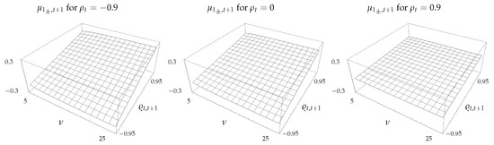
Figure 1. Expected CSM return, ${\mu }_{1_{\pm },t+1}$, as a function of $\nu$ and ${\varrho }_{t,t+1}$.

The standard deviation of the CSM return as a function of $\nu$ and ${\varrho }_{t,t+1}$ is shown in Figure 2. Although not clearly evident from the figure, ${\sigma }_{1_{\pm },t+1}$ is a decreasing function of $\nu$, and for a fixed value of $\nu$ the standard deviation is convex in ${\varrho }_{t,t+1}$ and takes the maximum value at ${\varrho }_{t,t+1}=0$. Finally, since the variance of the spread decreases as ${\rho }_t$ increases, ${\sigma }_{1_{\pm },t+1}$ likewise decreases with increasing ${\rho }_t$.

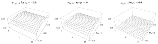
Figure 2. Standard deviation, ${\sigma }_{1_{\pm },t+1}$, of CSM return as a function of $\nu$ and ${\varrho }_{t,t+1}$.

The skewness of the CSM return in Figure 3 shows that ${\gamma }_{1_{\pm },t+1}$ is negative when ${\varrho }_{t,t+1}<0$ and positive otherwise. In fact, although it is not clearly evident from the figure, ${\gamma }_{1_{\pm },t+1}$ is negative even for small positive values of ${\varrho }_{t,t+1}$. As discussed above, the autocorrelations in the asset returns tend to be small in practice, and hence ${\varrho }_{t,t+1}$ will also be small. The corresponding model implied skewness in the CSM return will then be slightly negative, which is consistent with the observations in the empirical literature.

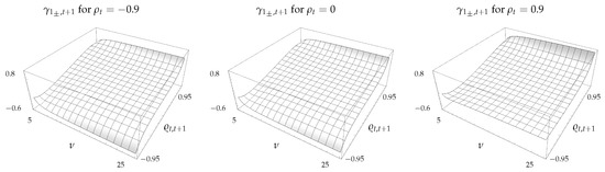
Figure 3. Skewness, ${\gamma }_{1_{\pm },t+1}$, of CSM return as a function of $\nu$ and ${\varrho }_{t,t+1}$.

In contrast to the surfaces for other quantities that flatten to a large extent as ${\rho }_t$ increases from $-0.9$ to $0.9$, the surface for ${\kappa }_{1_{\pm },t+1}$ in Figure 4 remains relatively unchanged. The excess kurtosis of CSM returns is generally positive, in line with the findings reported in the literature, and increases significantly when $\nu$ is small and $\left|{\varrho }_{t,t+1}\right|$ is high. It should be noted that ${\kappa }_{1_{\pm },t+1}$ is largest when $\nu$ is small. Since the deviation of the Student’s t distribution from the normal is greatest when $\nu$ is small, it follows that the extension considered in this paper will be useful in situations where the observed kurtosis in the CSM returns is higher than the value implied under the assumption of normal asset returns. This would be the case, for example, when considering emerging markets.

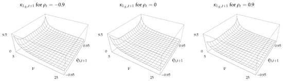
Figure 4. Excess kurtosis, ${\kappa }_{1_{\pm },t+1}$, of CSM return as a function of $\nu$ and ${\varrho }_{t,t+1}$.

5. Conclusions

In this paper, the theoretical framework introduced in Kwon and Satchell (2018) was extended to investigate the distributional properties of cross-sectional momentum (CSM) returns under the assumption that the vector of asset returns were multivariate Student’s t. The probability density function and the moments of the CSM returns were derived, and investigated in detail for the special case of two assets.

It was found that, in situations where the assets return, and hence the return spread, autocorrelations are small, and the CSM return has a small positive mean, negative skewness, and excess kurtosis. These are all consistent with the findings reported in the empirical literature. Moreover, the skewness and the kurtosis both become more pronounced as the number of degrees of freedom in the Student’s t distribution decreases and the corresponding asset returns become less normal.

In modeling asset returns that deviate significantly from being normal, such as those for emerging markets, the extension to the Student’s t considered in this paper would address some of the limitations of assuming normality. Since the Student’s t distribution approaches the normal in the limit as the number of degrees of freedom approaches infinity, the extension also provides a framework under which to analyze the implication and the limitations of the assumption of normality in asset returns to CSM returns.

References

- Arellano-Valle, Reinaldo B., and Adelchi Azzalini. 2006. On the Unification of Families of Skew-normal Distributions. Scandinavian Journal of Statistics 33: 561–74. [Google Scholar] [CrossRef]
- Arellano-Valle, Reinaldo B., and Marc G. Genton. 2010. Multivariate unified skew-elliptical distributions. Chilean Journal of Statistics 1: 17–33. [Google Scholar]
- Asness, Clifford S. 1994. Variables that Explain Stock Returns. Ph.D. dissertation, University of Chicago, Chicago, IL, USA. [Google Scholar]
- Asness, Clifford S., John M. Liew, and Ross L. Stevens. 1997. Parallels between the cross-sectional predictability of stock and country returns. Journal of Portfolio Management 23: 79–87. [Google Scholar] [CrossRef]
- Asness, Clifford S., Tobias J. Moskowitz, and Lasse H. Pedersen. 2013. Value and momentum everywhere. The Journal of Finance 58: 929–85. [Google Scholar] [CrossRef]
- Azzalini, Adelchi, and Alessandra Dalla Valle. 1985. The multivariate skew-normal distribution. Biometrika 83: 715–26. [Google Scholar] [CrossRef]
- Bekaert, Geert, Claude B. Erb, Campbell R. Harvey, and Tadas E. Viskanta. 1997. What Matters for Emerging Equity Market Investments. Emerging Markets Quarterly 1: 17–46. [Google Scholar]
- Carhart, Mark M. 1997. On Persistence in Mutual Fund Performance. Journal of Finance 52: 57–82. [Google Scholar] [CrossRef]
- Chan, Kalok, Allaudeen Hameed, and Wilson Tong. 2000. Profitability of Momentum Strategies in the International Equity Markets. Journal of Financial and Quantitative Analysis 35: 153–72. [Google Scholar] [CrossRef]
- Daniel, Kent, and Tobias J. Moskowitz. 2016. Momentum Crashes. Journal of Financial Economics 122: 221–47. [Google Scholar] [CrossRef]
- Erb, Claude B., and Campbell R. Harvey. 2006. The strategic and tactical value of commodity futures. Financial Analysts Journal 62: 69–97. [Google Scholar] [CrossRef]
- Fama, Eugene, and Kenneth French. 1992. The Cross-Section of Expected Stock Returns. The Journal of Finance 47: 427–65. [Google Scholar] [CrossRef]
- Hameed, Allaudeen, and Kusnadi Yuanto. 2002. Momentum Strategies: Evidence from the Pacific Basin Stock Markets. Journal of Financial Research 25: 383–97. [Google Scholar] [CrossRef]
- Hansen, Christian, James B. McDonald, and Whitney K. Newey. 2010. Instrumental Variables Estimation with Flexible Distributions. Journal of Business and Economic Statistics 28: 13–25. [Google Scholar] [CrossRef]
- Israel, Ronen, and Tobias J. Moskowitz. 2013. The Role of Shorting, Firm Size, and Time on Market Anomalies. Journal of Financial Economics 108: 275–301. [Google Scholar] [CrossRef]
- Jamalizadeh, Ahad, and Narayanaswamy Balakrishnan. 2012. Concomitants of order statistics from multivariate elliptical distributions. Journal of Statistical Planning and Inference 142: 397–409. [Google Scholar] [CrossRef]
- Jegadeesh, Narasimhan, and Sheridan Titman. 1993. Returns to buying winners and selling losers: Implications for stock market efficiency. The Journal of Finance 48: 65–91. [Google Scholar] [CrossRef]
- Jegadeesh, Narasimhan, and Sheridan Titman. 2001. Profitability and Momentum Strategies: An Evaluation of Alternative Explanations. Journal of Finance 56: 699–720. [Google Scholar] [CrossRef]
- Kan, Raymond. 2008. From moements of sum to moments of product. Journal of Multivariate Analysis 99: 542–54. [Google Scholar] [CrossRef]
- Kirkby, Justin L., Dang Nguyen, and Duy Nguyen. 2019. Moments of Student’s t-distribution: A Unified Approach. arXiv arXiv:1912.01607. [Google Scholar] [CrossRef]
- Kwon, Oh Kang, and Stephen Satchell. 2018. The distribution of cross sectional momentum returns. Journal of Economic Dynamics and Control 94: 225–41. [Google Scholar] [CrossRef]
- Lewellen, Jonathan. 2002. Momentum and autocorrelation in Stock Returns. Review of Financial Studies 15: 533–63. [Google Scholar] [CrossRef]
- Lo, Andrew, and Craig MacKinlay. 1990. When are Contrarian Profits due to Stock Marjket Overreaction? Review of Financial Studies 3: 175–205. [Google Scholar] [CrossRef]
- Menkhoff, Lucas, Lucio Sarno, Maik Schmeling, and Andreas Schrimpf. 2012. Currency momentum strategies. Journal of Financial Economics 106: 660–84. [Google Scholar] [CrossRef]
- Moskowitz, Tobias J., Yao Hua Ooi, and Lasse H. Pedersen. 2012. Time Series Momentum. Journal of Financial Economics 104: 228–50. [Google Scholar] [CrossRef]
- Muirhead, Robb J. 1982. Aspects of Multivariate Statistical Theory. New Jersey: John Wiley & Sons. [Google Scholar]
- Okunev, John U., and Derek White. 2003. Do momentum-based strategies still work in foreign currency markets? Journal of Financial and Quantitative Analysis 38: 425–47. [Google Scholar] [CrossRef]
- Richards, Anthony J. 1997. Winner-Loser Reversals in National Stock Market Indices: Can They be Explained? Journal of Finance 52: 2129–44. [Google Scholar] [CrossRef]
- Roth, Michael. 2013. On the Multivariate t-Distribution. Technical Report. Linköping: Department of Electrial Engineering, Linköpings Universitet. [Google Scholar]
- Rotman, Joseph J. 1995. An Introduction to the Theory of Groups. New York: Springer. [Google Scholar]
- Rouwenhorst, Geert K. 1998. International Momentum Strategies. Journal of Finance 53: 267–84. [Google Scholar] [CrossRef]
- Rouwenhorst, Geert K. 1999. Local Return Factors and Turnover in Emerging Stock Markets. Journal of Finance 54: 1439–64. [Google Scholar] [CrossRef]
- Sefton, James, and Alan Scowcroft. 2004. A Decomposition of Portfolio Momentum Returns. Discussion Paper TBS/DP04/9. London: Tanaka Business School, Imperial College London. [Google Scholar]
- Theodossiou, Panayiotis. 1998. Financial Data and the Skewed Generalized T Distribution. Management Science 44: 1650–61. [Google Scholar] [CrossRef]
- Withers, Christopher S. 1985. The Moments of the Multivariate Normal. Bulletin of Australian Mathematics Society 32: 103–7. [Google Scholar] [CrossRef]