Abstract
Systematic traders employ algorithmic strategies to manage their investments. As a result of the deterministic nature of such strategies, it is possible to determine their exact responses to any conceivable set of market conditions. Consequently, sensitivity analysis can be conducted to systematically uncover undesirable strategy behavior and enhance strategy robustness by adding controls to reduce exposure during periods of poor performance/unfavorable market conditions, or to increase exposure during periods of strong performance/favorable market conditions. In this study, we formulate both a simple systematic trend-following strategy (i.e., trading model) to simulate investment decisions and a market model to simulate the evolution of instrument prices. We then map the relationship between market model parameters under various conditions and strategy performance. We focus, in particular, on identifying the performance impact of changes in both serial dependence in price variability and changes in the trend. The long-range serial dependence of the true range worsens performance of the simple classic trend-following strategy. During periods of strong performance, the dispersion of trading outcomes increases significantly as long-range serial dependence increases.
1. Introduction
For the class of market participants employing fully systematic approaches to manage their investments, it is possible to estimate the outcomes of their strategies in response to any conceivable set of market conditions. Sensitivity analysis may uncover undesirable strategy behavior and can be used to enhance strategy robustness.
Systematic traders often use sensitivity analysis to identify the set conditions under which the trading system will operate within acceptable bounds. In this study, we refer to this set of conditions as the operational domain of the strategy (for a specific set of trading model parameters). The broader the spectrum of market conditions over which a trading system can perform within acceptable performance bounds (i.e., the broader the operational domain of the strategy), the more robust the trading system.
In general, the operational domain of a trading strategy can be broadened through the introduction of feedback and feed-forward risk controls. Feedback risk controls operate to reduce the impact of unpredictable phenomena or events on strategy performance, while feed-forward controls exploit regularities in market structure to make local predictions that aid in the enhancement of strategy performance. We use feedback controls when poor trading performance is not driven by something we can predict. We use feed-forward controls when we understand the drivers of poor performance and there is enough persistence in the market conditions for us to effectively anticipate future poor performance.
In the following sections, a simple systematic investment approach—a so called trend-following strategy (Hurst et al. 2017)—is explored through the use of Monte Carlo simulation. In particular, a market model is specified and used to generate realistic realizations of financial instrument prices across of broad spectrum of market conditions. Sensitivity analysis is then conducted, mapping the relationship between market model parameters and the strategy performance under a particular set of trading model parameters.
The market model (i.e., the model used to simulate instrument prices) has been designed to capture a set of essential stylized facts believed to be critical to the effective functioning of the strategy. As a model is a simplification of reality by definition, we do not attempt to reproduce all empirical stylized facts. We limit the complexity and scope of the work by focusing on the instrument-level strategy. Portfolio-level meta-strategies that determine how to allocate across instrument-level strategy instances are not explored.
Typically, systematic traders backtest the strategies that they employ (i.e., they use historical data to evaluate potential performance). Such backtesting allows systematic traders to determine the response of a strategy to the exact mix of market conditions that actually occurred, but not the response of a strategy to conditions that have not yet occurred, or that may occur in different proportions in the future (De Prado 2018). Typically, the longer the historical period used, the more varied the market conditions, and the more likely that historical data can be used to build a relatively complete picture of the operational domain.
There are two main ways to supplement the historical data available for testing, namely market model-based Monte Carlo simulation, and Monte Carlo resampling. In this study, we focus on the former approach to explore the characteristics of a simple trend-following strategy.
In order to simulate financial prices, a market model is designed, implemented, and calibrated to financial market data. The market model reproduces key well-established stylized facts, particularly focusing on time-varying, serially dependent price variability. Trading strategy sensitivities are created by simulating price and true range scenarios—consisting of many realizations—for a range of key market model parameters, then computing the performance of the trading strategy for all realizations under each scenario.
The paper is motivated by the need for decision support tools that can be used to improve the robustness of systematic trading systems and by the lack of literature addressing this key aspect of the work of systematic investors. By using the methods in this study, a systematic investor may evaluate the performance of different trading strategies against varying market conditions. The application of this technique is likely to lead to improved systems that are more robust to market changes.
Stylized Facts
There exists a vast literature on the empirical characteristics of financial markets, documenting extensively the basic stylized facts. A similarly broad literature also exists on the derivation of financial derivative sensitivities. To price and risk manage products with path-dependent payoffs similar to a trend-following strategy, Monte Carlo simulation is often required. Despite a seemly obvious link between the analysis of systematic trading strategies and the analysis of replication strategies used to manufacture financial derivative products, little published work exists leveraging the findings in these two areas of research to the analysis of systematic trading strategies.
Although the scope of this study does not allow for a detailed exploration of the stylized facts, a number of comprehensive surveys exist (Bollerslev et al. 1992; Brock and de Lima 1996; Pagan 1996; Cont 2001; Farmer and Geanakoplos 2009; Gourieroux and Jasiak 2001; Rao and Maddala 1996; Pagan 1996; Shephard 1996). The most basic and commonly agreed upon facts upon which we rely in this study are as follows: (1) price returns of financial instruments are not serially correlated whereas return variability is; (2) the unconditional distributions of returns are heavy-tailed, and; (3) price variability for all financial instruments is time-varying.
Figure 1 provides an example of the insignificant log return serial correlation with significant true-range serial correlation (first stylized fact). Notice that the autocorrelation of the true range decays very slowly. A similar pattern is found for all common measures of price variability. In the model calibration section, we outline the scaling law that describes the pattern in the autocorrelation and specify a model to simulate this behavior.
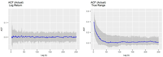
Figure 1.
First stylized fact.
Heavy right-tailed distributions, P(X > x), are those distributions with tails that decay slower than an exponential distribution. The definition for a heavy left-tail distribution is analogous, P(X < −x). A log-normal distribution is a heavy-tailed distribution. Figure 2 illustrates for three instruments in the data set that their shapes are approximately log-normal. A similar pattern is found for the log returns of all global futures instruments studied herein.
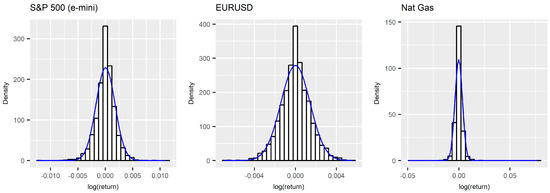
Figure 2.
Second stylized fact.
The third stylized fact indicates that price variability of instruments is time-varying. Figure 3 shows the true range of the same instruments in Figure 2. That variability is non-constant over time, and the pattern persists across the global futures instruments studied.
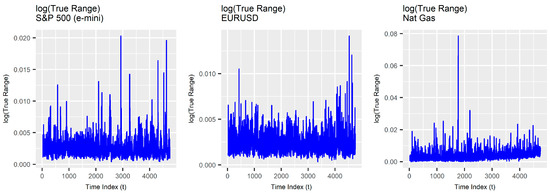
Figure 3.
Third stylized fact.
2. Materials and Methods
2.1. Data Acquisition and Transformation
Futures contracts for 115 distinct markets over the period between 1 January 1999 and 5 May 2017 were acquired from Commodity Systems Incorporated (CSI). For each instrument, a back-adjustment process was used to build a continuous series, then a volatility-normalized total return index accounting for changes in prices and the impact of ‘rolls’ was constructed. It is important to note that the total return of a long-term position taken using futures instruments must account for so-called ’rolls’. As futures contracts have finite maturities, to take a long-term position, a trader must trade a series of individual futures contracts. Traders must repeatedly extend the maturity of their positions by executing spread trades that close positions nearing expiry and open equivalent positions in contracts with greater maturity. The process of converting a position about to expire into a position with an expiry further into the future (thereby extending the maturity) is commonly referred to as a ’roll’. The maturity profile associated with particular roll parameters is an important determinant of total return in futures-based strategies.
Figure 4 depicts the total return index for each of the global futures markets in the upper half of the figure and the corresponding true range for the volatility-normalized total return indices in the lower half. The true range is a commonly used measure of the daily price range of a financial instrument that accounts for gaps from the close of the previous period to the opening of the current period (Equation (1)) where Pt,H and Pt,L are the current daily high and low prices respectively, and Pt−1 is the previous closing price.
Rt = max[Pt,H − Pt,L, |(Pt,H − Pt−1)|, |(Pt,L − Pt−1)|]
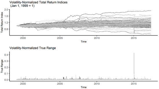
Figure 4.
Global futures volatility normalized return indices and true range.
The index for each instrument represents the total return on a re-balanced position sized to equate a move of four units of price variability (i.e., average true range) to a 1% loss. Positions are rebalanced at each roll. Use of the volatility-normalized total return index facilitates comparison of model parameters across the instrument universe and was also used to meet the data agreement conditions of the vendor.
2.2. Software
This study leveraged the R bookdown package (Xie 2016), which was built on top of R Markdown and knitr (Xie 2015). All of the code used to generate this study is available on the project github page: https://github.com/dgn2/IS609. The file descriptions follow.
- buildGlobalFuturesDataset.R: Extracts data from a MySQL database and builds the R data set.
- establishStylizedFacts.R: Used to explore the stylized facts.
- calibrateMarketModelLRD_log.R: Calibrates the market model.
- selectTradingModelParameters.R: Used to explore the trading model parameters via brute force search.
- simulateMarketModelLRD_rerun_2.R: Simulates the market model and computes the sensitivities.
As a single run of the simulation produces nearly 28 gigabytes of data, it is not possible to make the full result set available on github. Key results and data have been uploaded to github. The project R Markdown files (.Rmd) assemble the visualization and text comprising the study.
2.3. Market Model Specifications
We define and use a simple discrete time model to simulate a broad set of market conditions. Each scenario consists of realizations of both price and true range. Equation (2) is the discrete time process used to generate price realizations for a single instrument. In this equation, t = 1 … T, ∆t = 1/T, ϵt ~ N(0,1), σt is the time-varying volatility, and μ is the constant drift for the instrument over time period, T.
Pt = Pt−1exp(μΔt + σtϵt)
The volatility is a function of the observed true range, Rt (Chou 2005) as shown in Equation (3).
σt = (π/8)5 × Rt
Similar to the work of (Chou 2005; Brunetti and Lildholdt 2007), we extend a model originally designed for the modeling of duration time series to a time-varying price range. Following (Beran et al. 2015), the true range at time, t, is given by Equation (4). In this equation, v is a scale parameter (v > 0), λt is the conditional mean of the true range (λt > 0) divided by v, and ηt is an independent and identically distributed (i.i.d) log-normal random variable.
Rt = vλtηt
After subtracting the unconditional mean, log(v), the log true range is represented as a zero mean FARIMA(p,d,q) process (Equation (5)) with innovations e = log(ηt), given by Equation (6). In Equation (6), d is the long memory parameter (0 < d < 0.5); B is the back-shift (or lag operator); and ϕ(z) =1 − ϕ1z − … ϕpzp, ψ(z) = 1 + ψ1 + … + ψqzq are MA- and AR-polynomials with all roots outside the unit circle. The back-shift operator is used for notational convenience where Bmxt = xt=m. This notation allows (even infinite) distributed lags to be represented concisely.
Zt = log(Rt) − log(v) = log(λt) + et
(1 − B)dϕ(B)Zt = ψ(B)et
Denoting log(λt) as ζt and rearranging, we can see that the conditional mean of Zt yields Equation (7), where E(ζt) = 0.
ζt = log(λt) = [ϕ−1(B)ψ(B)(1 − B)−d − 1]et
The autocorrelations of Zt exhibit a hyperbolic decay (Figure 2), the speed of which depends upon the parameter d as in Equation (8) where cpZ > 0 is a constant.
ρ(k) ~ cpZ|k|2d − 1
The general class of models defined by Equations (5) and (6) are referred to as exponential FARIMA (EFARIMA) models (Beran et al. 2015). Where et are normally distributed, the model is referred to as a Gaussian EFARIMA model. Setting p = 0 and q = 0, the innovations, e = log(ηt), simplifies to Equation (9).
(1 − B)dZt = et
This simpler specification is particularly useful for sensitivity analysis.
Our market model has two sources of uncertainty, namely ϵ and e. Bursts in volatility driven by the true range process can generate price momentum that looks very similar to that observed in real markets.
2.4. Market Model Calibration
For each instrument in the universe under study, we fit an EFARIMA(0,d,0) model with log-normal errors. We then use the cross-section of parameters to define the starting range of parameters for use in our sensitivity analysis.
Given the definition of our market model (defined above), we observe two processes: Pt and Rt. We assume that Rt (t = 1, 2, …, T) is generated by an EFARIMA process with an unknown parameter vector in Equation (10).
θ = (v, σe2, d, ϕ1, …, ϕp, ψ1, …, ψq)T
For the EFARIMA(0,d,0) model, this parameter set reduces to Equation (11).
θ = (v, σe2, d)T
Since Zt = log(Rt) − log(v) is a centered Gaussian FARIMA process, maximum likelihood estimation (MLE) can be used to estimate the parameters (Mills 1999; Fox and Taqqu 1986; Giraitis and Surgailis 1990; Beran 1995; Haslett and Raftery 1989). This allows us to use standard, widely-available, estimation software to calibrate the model (McLeod et al. 2007; Veenstra and McLeod 2015). We assume that the price process is a function of the volatility, which is in turn a function of Rt and employ the ARFIMA R package (Veenstra and McLeod 2015) to estimate the parameters of true range for each instrument in the universe under study (Appendix A). For the vast majority of the instruments in the universe under study, the estimated d parameter is between 0.15 and 0.35. All parameters are highly significant.
The EFARIMA(0,d,0) model for the true range provides a framework for forecasting the conditional mean true range. These predictions could replace the EMA smoothed true range in the simple trend-following system, potentially significantly improving the effectiveness of the position-sizing and trailing stop loss components of the trading system.
From Figure 5, it is evident that model residuals retain some short-term memory, suggesting that a EFARIMA(p,d,q) model could provide a better fit. To reduce the dimension of our sensitivity analysis, we use the simpler model (recognizing that it captures the broader long memory but could likely be improved with a higher order model).
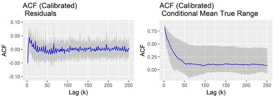
Figure 5.
ACF residuals.
Using the market model, we simulate a single price and true range path for each instrument and plot the results to provide an intuitive means of checking the realism of the model (Figure 6). The simulated paths appear similar to the actual paths depicted previously.
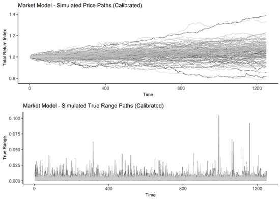
Figure 6.
Market model simulated paths (calibrated to global futures).
2.5. Trading Model Specifications
We implement a very simple version of a common systematic trend-following strategy (Curtis 2007). The instrument-level logic of the trading system has several core components: (1) The entry signal, determines timing for initiating a position (either long or short) in a particular instrument; (2) The position sizing algorithm determines the size of a position; and, (3) The trailing stop loss determines the timing of an exit from a position. Both the position size and the distance of the trailing stop from the current price level are functions of the true range, Rt. Filters are commonly used to smooth price series. We use exponentially weighted moving averages (EMAs) to smooth both price and the true range time series. The core rules of our simple trading model are detailed briefly in the next two sub-sections.
2.5.1. Long Position
At t, if the fast EMAt−1,F is above the slow EMAt−1,S and we have no position, we enter a long position of pt units (Equation (12)).
pt = floor[f At−1 ÷ max[ATRt−1 × M, L]]
Here, f is the fraction of account size plus accrued realized P&L risked per bet (A), ATRt−1 is the EMA of the true range for the previous time step, M is the risk multiplier, and L is the ATR floor.
We set our initial stop loss level M units of ATR below the entry price level, pt. For each subsequent time, t, we update our stop level as in Equation (13).
st = max[Pt − ATRt−1 × M, st−1]
We exit our long position if the price, pt moves below the stop loss level, st−1.
2.5.2. Short Position
At t, if the fast EMAt−1,F is below the slow EMAt−1,S and we have no position, we enter a short position of pt units (Equation (14)).
pt = −floor[f At−1 ÷ max[ATRt−1 × M, L]]
We set our initial stop loss level M units of ATR above the entry price level, pt. For each subsequent time, t, we update our stop level as in Equation (15).
st = min[Pt + ATRt−1 × M, st−1]
Regardless of whether we are long or short, for each trade we budget for a loss of f percent of our account size plus accrued realized P&L. The effectiveness of this crude risk budgeting system is a function of the characteristics of the true range. Serial dependence in the true range can transform this simple mechanism from a feedback control to a feed-forward control.
3. Results
3.1. Parameter Selection
The selection of robust trading model parameters is a complex process. Typically, bootstrapping inputs, determining the trading model performance for each bootstrapped path for each coordinate in the parameter space, then averaging the results for each coordinate in the parameter space, vastly improves the continuity of the space for visualization. Given the computationally intensive nature of such a task, this type of process can only be achieved through the use of parallel processing. We use a brute force grid search to get a course understanding of the parameter space.
We first examine the impact of the ATR multiplier on the geometric mean return (Figure 7). Our interest is not in finding the absolute highest performance, but in selecting a parameter that both performs well and is located in a reasonably stable part of the parameter space. We select a multiplier of 4, then search the EMA lookback space. We also select a fast lookback of 120 and a slow lookback of 180 days based on careful evaluation of the results based on graphical analysis.
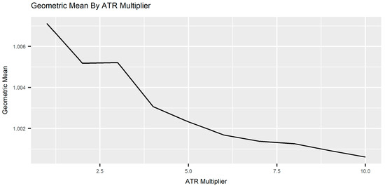
Figure 7.
Performance impact of ATR multiplier.
3.2. Sensitivity Analysis
Previously, we specified a market model and calibrated it to each instrument in the global futures universe under study. We then outlined the rules of a simple trading strategy and explored the parameter space. Now, we use the market and trading models to create sensitivities.
The parameter space of the combined market and trading models is vast. To reduce the dimension of the problem, an initial study was conducted to coarsely explore the impact of different trading model parameters on the strategy backtest results (Section 3.1). A set of trading model parameters was selected from stable areas of the response curves.
Following the selection of the trading model parameters, the range of market parameters observed over the entire instrument universe under study was examined and used to determine realistic starting parameter ranges for sensitivity analysis. These ranges were then extended to account for realistic conditions that may be observed in in the future. Once ranges were selected, another coarse study was conducted to determine which market model parameters had the largest impact on performance. Based on these results, the drift (μ) and d parameters were selected for the final sensitivity analysis. Exactly 1000 paths, each with a 1250 day length (roughly 5 years), were used for all simulations. The strategy performance measure (TWR) is defined in Appendix B. A single sensitivity simulation run varying only the drift and d parameters, but holding all other variables constant, generates just under 28 gigabytes of simulated market model input and trading model output.
Table 1 shows the parameters that are held fixed for the simulations in this Chapter. The drift (μ) is varied by 0.005 between −0.1 and 0.1. The long memory parameter (d) is varied by 0.05 between 0.05 and 0.45.

Table 1.
Parameter values.
3.2.1. Trend Sensitivity
Trend-following strategies operate on the premise that the emergence of a trend in a particular instrument cannot be predicted. The system is designed to maintain a position in an instrument as long as it is trending and exit the position when the trend has reversed beyond a multiple of the typical daily range. Any predictability in the characteristics of true range, is thus expected to enable strategy enhancement.
First we use our market model defined above to determine the sensitivity of the strategy to trends of different magnitudes by computing trading model performance under different drift rates (μ). The profile that emerges from this sensitivity analysis of the strategy performance with respect to changes in the drift (μ) illustrates the essence of the strategy (Figure 8). From the profile, it is clear that as the price moves up or down strongly, the strategy performance increases. The less variability around the trend, the better the strategy’s performance. Choppy, sideways movement in prices produces a condition where the strategy repeatedly enters and gets stopped out, generating losses for roughly half of the paths. Increasing the strength of long range dependence in true range by increasing d increases the dispersion of results, particularly for very favorable trend conditions (i.e., high drift, μ).
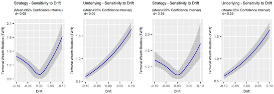
Figure 8.
Profile of trend sensitivity.
Examining sample price paths with the trailing stop and signal superimposed, it is possible to get some intuition about the result. As we increase the strength of long memory in the true range, the price paths get visibly more volatile (Figure 9). The stop is the blue line that ratchets behind the price depicted in black. The red line shows the fast EMA, while the purple line depicts the slow EMA. As we reduce the drift (in absolute value terms), the strategy gets stopped out more often. Performance is better on the long side than the short side because price is unbounded on the positive side, but bounded by zero on the negative side.
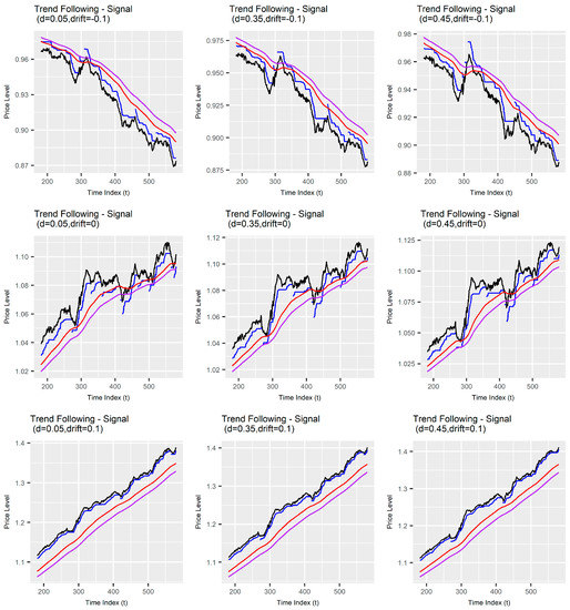
Figure 9.
Volatility of price paths.
Focusing on the terminal wealth relative curves (See Appendix B for details), one can see that increasing variation around the trend reduces performance (Figure 10). The impact of increasing d is largest during strong trend conditions.
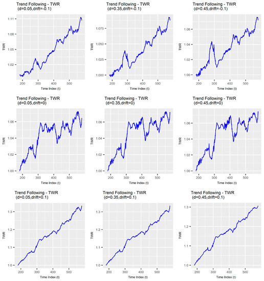
Figure 10.
Terminal wealth relative (TWR) curves.
3.2.2. Serial Dependence in True Range Sensitivity
Given the observed long range serial dependence in the true range, a natural question arises as to the sensitivity of the performance of our simple trading model to the strength of autocorrelation. To determine the link between strategy performance and autocorrelation we perturb the d parameter, generate price and true range scenarios, then evaluate strategy performance under each scenario.
Counter-intuitively, increasing the long range dependence in the true range increases the dispersion of outcomes, and for the most part worsens performance. There is a slight improvement in both median and mean performance as long range dependence decreased. Although it is difficult to determine the source of this effect without a significant amount of additional research, it seems likely that it is possible to redesign components of the trading system to exploit the regularity in true range driven by long range dependence. The model that has been developed in this report should provide a reasonable starting point for such an endeavor.
4. Discussion
In this study, we formulated both a simple systematic trend-following strategy (i.e., trading model) to simulate investment decisions, and a market model to simulate the evolution of instrument prices. We explored the sensitivity of our strategy to different market conditions (for a particular set of trading model parameters) and provided a map between the market model parameters for each scenario representing a particular market condition and strategy performance. In particular, we focused on identifying the performance impact of changes in (1) serial dependence in price variability, and; (2) changes in the trend.
The sensitivities derived provide an effective visual depiction of the fundamental profile of the simple trading strategy and suggest an explanation for the functions of trading model components commonly found in trend-following strategies. The long-range serial dependence in the true range appears to worsen performance of the simple classic trend-following strategy. During periods of strong performance, the dispersion of trading outcomes increases significantly as long-range serial dependence increases.
In this study, we are evaluating only one trading strategy based on paths generated by a particular market model formulation. This is a clear limitation of the work. A systematic trader is likely to evaluate multiple strategies against both simulated and actual market conditions to evaluate performance and then conduct robustness checks under various simulated and observed market conditions.
More research is required to determine whether a slightly more complex feed-forward controller could be created to improve the performance of the strategy by exploiting long memory in the true range. An extension of our simple single instrument market model to a multiple instrument model could provide useful sensitivity analysis relating to the cross-dependence between instruments.
The methods and overall algorithm provided in this study may be used by investors to evaluate any systematic trading strategy. In doing so, investors may compare the performance of different trading systems under varying market conditions—including those that have not been observed historically. Application of this technique is likely to improve the robustness of an investor’s trading system.
Author Contributions
Conceptualization, D.N. Validation: L.F.
Funding
This research received no external funding.
Conflicts of Interest
The authors declare no conflict of interest.
Appendix A
| Item # | Instrument Name | d | log(V) | var(e) | mu |
| 1 | Brent Crude Oil | 0.2355 | −6.2819 | 0.1489 | 0.0092 |
| 2 | Crude Oil | 0.2209 | −6.3405 | 0.17 | 0.0122 |
| 3 | Ethanol | 0.2809 | −6.7159 | 0.4139 | 0.0571 |
| 4 | Gas Oil | 0.2198 | −6.3044 | 0.1542 | 0.0096 |
| 5 | Gas-RBOB | 0.2011 | −6.1794 | 0.1672 | 0.0022 |
| 6 | Heating Oil | 0.2449 | −6.2499 | 0.1439 | 0.0099 |
| 7 | Nat Gas | 0.2886 | −6.14 | 0.1594 | −0.0022 |
| 8 | WTI Crude Oil | 0.2177 | −6.2201 | 0.3278 | −0.0024 |
| 9 | ECX EUA Emissions | 0.3822 | −5.7152 | 0.1031 | −0.0142 |
| 10 | Nat Gas | 0.372 | −5.8487 | 0.4072 | −0.0386 |
| 11 | AUDUSD | 0.2638 | −6.185 | 0.14 | 0.0067 |
| 12 | CADUSD | 0.2694 | −6.1393 | 0.1334 | 0.002 |
| 13 | CHFUSD | 0.2222 | −6.1448 | 0.1587 | 0.0034 |
| 14 | EURUSD | 0.2132 | −6.1638 | 0.1455 | 0.0014 |
| 15 | GBPUSD | 0.2373 | −6.1258 | 0.1397 | 0.0004 |
| 16 | JPYUSD | 0.2847 | −6.0951 | 0.1754 | −0.0058 |
| 17 | NZDUSD | 0.183 | −6.2719 | 0.3233 | 0.0123 |
| 18 | US Dollar Index | 0.183 | −6.0317 | 0.1807 | −0.0018 |
| 19 | EURCHF | 0.3317 | −6.1226 | 0.5683 | −0.0181 |
| 20 | EURGBP | 0.203 | −5.9885 | 0.4755 | −0.0013 |
| 21 | EURJPY | 0.2507 | −6.35 | 0.4758 | 0.0084 |
| 22 | BRLUSD | 0.2252 | −6.5292 | 0.7088 | 0.0223 |
| 23 | CZKUSD | 0.0844 | −6.5137 | 1.1831 | −0.0043 |
| 24 | HUFUSD | 0.0897 | −6.4835 | 1.1712 | −0.0073 |
| 25 | MXNUSD | 0.3382 | −6.1907 | 0.1611 | 0.005 |
| 26 | PLNUSD | 0.1315 | −6.5222 | 1.1359 | 0.0062 |
| 27 | RUBUSD | 0.2953 | −6.163 | 0.3264 | 0.0046 |
| 28 | ZARUSD | 0.1748 | −6.2179 | 0.6859 | −0.0049 |
| 29 | USDKRW | 0.273 | −6.0789 | 0.2116 | −0.0022 |
| 30 | Corn | 0.3198 | −6.0545 | 0.172 | −0.0009 |
| 31 | Oats | 0.3307 | −6.2312 | 0.2129 | 0.0118 |
| 32 | Rough Rice | 0.286 | −6.0389 | 0.208 | −0.0084 |
| 33 | Soybean Meal | 0.3132 | −6.322 | 0.1647 | 0.0203 |
| 34 | Soybean Oil | 0.244 | −6.1338 | 0.1459 | 0.0053 |
| 35 | Soybeans | 0.2783 | −6.2305 | 0.1561 | 0.0164 |
| 36 | Wheat | 0.2748 | −6.0158 | 0.1416 | −0.0066 |
| 37 | Corn | 0.286 | −6.5743 | 0.6159 | 0.0274 |
| 38 | Milling Wheat | 0.3447 | −6.5546 | 0.6575 | 0.0339 |
| 39 | Rapeseed | 0.2804 | −6.5859 | 0.5275 | 0.0166 |
| 40 | Wheat | 0.3195 | −6.2202 | 0.4898 | 0.0065 |
| 41 | Dow Jones Industrial (mini) | 0.3304 | −6.1172 | 0.1621 | 0.0105 |
| 42 | MSCI EAFE (mini) | 0.3136 | −6.1508 | 0.2195 | 0.01 |
| 43 | Nasdaq 100 (e-mini) | 0.3325 | −6.1532 | 0.1491 | 0.0136 |
| 44 | Russell 2000 (mini) | 0.3029 | −6.1539 | 0.1477 | 0.0125 |
| 45 | SP 500 (e-mini) | 0.3359 | −6.1039 | 0.1596 | 0.0089 |
| 46 | Belgian 20 | 0.239 | −6.0888 | 0.2724 | 0.0123 |
| 47 | CAC 40 | 0.293 | −6.1944 | 0.1899 | 0.007 |
| 48 | DAX | 0.2998 | −6.2708 | 0.2117 | 0.0081 |
| 49 | DJ Euro STOXX 50 | 0.309 | −6.0845 | 0.1636 | 0.0058 |
| 50 | EOE (Amsterdam) | 0.2994 | −5.9945 | 0.1449 | 0.0028 |
| 51 | FTSE 100 | 0.3368 | −5.9297 | 0.1181 | 0.004 |
| 52 | IBEX 35 | 0.2771 | −6.2074 | 0.1749 | 0.0072 |
| 53 | MIB FTSE | 0.3057 | −6.2135 | 0.1974 | 0.0011 |
| 54 | Nikkei 225 | 0.2941 | −6.3303 | 0.3148 | 0.0055 |
| 55 | OMX | 0.386 | −6.9382 | 0.165 | 0.0124 |
| 56 | SPTSE 60 | 0.2485 | −6.0678 | 0.1485 | 0.0113 |
| 57 | SMI | 0.3235 | −5.9756 | 0.1364 | 0.008 |
| 58 | SPI 200 | 0.2745 | −6.3048 | 0.2375 | 0.0099 |
| 59 | TOPIX | 0.2845 | −6.2746 | 0.2545 | 0.0074 |
| 60 | MSCI EM (mini) | 0.2801 | −6.0982 | 0.1943 | −0.0027 |
| 61 | MSCI Taiwan | 0.2195 | −6.1515 | 0.1817 | 0.0092 |
| 62 | SP CNX Nifty | 0.1867 | −6.3298 | 0.4275 | 0.0175 |
| 63 | Hang Seng | 0.1864 | −6.2192 | 0.1769 | 0.0128 |
| 64 | Hang Seng (mini) | 0.1814 | −6.1844 | 0.1782 | 0.0128 |
| 65 | Hang Seng China Enterprises | 0.2633 | −6.2258 | 0.153 | 0.0158 |
| 66 | IPC | 0.3258 | −5.8855 | 0.1262 | 0.0064 |
| 67 | KOSPI 200 | 0.2357 | −6.5445 | 0.4424 | 0.0126 |
| 68 | Feeder Cattle | 0.2522 | −6.1331 | 0.1549 | 0.0109 |
| 69 | Lean Hogs | 0.2451 | −5.9264 | 0.1445 | −0.0064 |
| 70 | Live Cattle | 0.2083 | −6.1276 | 0.1491 | 0.0088 |
| 71 | Copper | 0.2635 | −6.1975 | 0.1522 | 0.0091 |
| 72 | Gold | 0.3005 | −6.18 | 0.1894 | 0.0108 |
| 73 | Palladium | 0.3813 | −6.2387 | 0.2212 | 0.0111 |
| 74 | Platinum | 0.3442 | −6.2491 | 0.1652 | 0.011 |
| 75 | Silver | 0.3047 | −6.1876 | 0.1795 | 0.0066 |
| 76 | USD Deliverable Swap 10 year | 0.299 | −6.0867 | 0.208 | 0.0123 |
| 77 | USD Deliverable Swap 5 year | 0.2849 | −6.0717 | 0.2412 | 0.007 |
| 78 | USD Govt 10yr | 0.2797 | −6.2127 | 0.1532 | 0.0173 |
| 79 | USD Govt 15–30yr | 0.2606 | −6.1806 | 0.1457 | 0.0141 |
| 80 | USD Govt 2yr | 0.2951 | −6.2539 | 0.1923 | 0.0209 |
| 81 | USD Govt 30yr | 0.3198 | −6.1727 | 0.1455 | 0.0156 |
| 82 | USD Govt 5yr | 0.2751 | −6.2401 | 0.1649 | 0.0176 |
| 83 | AUD Govt 10yr | 0.1748 | −6.3502 | 0.3921 | 0.0076 |
| 84 | AUD Govt 3yr | 0.1689 | −6.3336 | 0.4123 | 0.0084 |
| 85 | CAD Govt 10yr | 0.2198 | −6.1027 | 0.2192 | 0.0182 |
| 86 | CHF Govt 10yr | 0.2652 | −6.3925 | 0.3511 | 0.02 |
| 87 | DEM Govt 10yr | 0.2364 | −6.4194 | 0.2785 | 0.0172 |
| 88 | DEM Govt 2yr | 0.2896 | −6.3881 | 0.3155 | 0.0179 |
| 89 | DEM Govt 5yr | 0.2472 | −6.4036 | 0.2799 | 0.0186 |
| 90 | FRF Govt 10yr | 0.3146 | −6.098 | 0.1477 | 0.0307 |
| 91 | GBP Govt 10yr | 0.2338 | −6.0316 | 0.1308 | 0.0132 |
| 92 | ITL Govt 10yr | 0.4065 | −5.9488 | 0.1303 | 0.0201 |
| 93 | ITL Govt 2yr | 0.4559 | −6.019 | 0.2678 | 0.0294 |
| 94 | JPY Govt 10yr (mini) | 0.3342 | −6.3402 | 0.2904 | 0.0182 |
| 95 | KRW Govt 10yr | 0.295 | −6.3422 | 0.2746 | 0.0275 |
| 96 | Butter | 0.2603 | −6.0707 | 0.8538 | 0.0164 |
| 97 | Cocoa | 0.2437 | −6.11 | 0.1751 | 0.0011 |
| 98 | Coffee | 0.2895 | −6.0532 | 0.1854 | −0.0044 |
| 99 | Cotton 2 | 0.3031 | −6.1075 | 0.181 | −0.0023 |
| 100 | Lumber | 0.2773 | −5.9161 | 0.1449 | −0.0138 |
| 101 | Milk-Class III Fluid | 0.3337 | −6.1052 | 0.3525 | 0.0072 |
| 102 | Orange Juice | 0.2462 | −6.1736 | 0.2549 | 0.0069 |
| 103 | Robusta Coffee | 0.3565 | −6.0909 | 0.2177 | 0.0004 |
| 104 | Sugar 11 | 0.3112 | −6.2256 | 0.1673 | 0.0063 |
| 105 | Sugar 5 | 0.2975 | −6.2787 | 0.2071 | 0.0126 |
| 106 | TSR20 Rubber | 0.3321 | −6.1874 | 0.3907 | 0.0106 |
| 107 | Cocoa | 0.3086 | −5.9108 | 0.1417 | 0.0039 |
| 108 | USD STIR | 0.4512 | −6.1231 | 0.2431 | 0.0303 |
| 109 | AUD STIR | 0.2282 | −6.0767 | 0.3378 | 0.0081 |
| 110 | CAD STIR | 0.3843 | −5.9982 | 0.2806 | 0.0265 |
| 111 | CHF STIR | 0.4136 | −6.0595 | 0.2454 | 0.0332 |
| 112 | EUR STIR | 0.4227 | −5.7489 | 0.2022 | 0.0162 |
| 113 | GBP STIR | 0.33 | −5.9621 | 0.2374 | 0.0244 |
| 114 | VIX | 0.4345 | −5.9535 | 0.237 | −0.0443 |
| 115 | VSTOXX (mini) | 0.4162 | −5.9015 | 0.1454 | −0.0248 |
Appendix B
Evaluation Measures
In order to meet our objectives, we must have measures to quantify both strategy performance and the breadth of the operational domain.
We can define the terminal wealth relative as the multiplier that we apply to our starting equity to get our pending equity. In other words, the terminal wealth relative is the product of the accumulation rates (1 + return rate, Equation (A1)).
Here, rt is our return over period t, HPRt is our holding period return or one plus our return over the tth period, and TWRT is our terminal wealth relative or one plus our total return over T periods. We can approximate the return with Equation (A2).
Here, N is the number of sub-periods over which we have returns, aTWRT is the approximate terminal wealth relative (i.e., one plus the approximate total return over the T periods), and HPRt is the holding period return (i.e., the return over the tth period).
AHPRT is arithmetic average of the holding period returns over the T periods (Equation (A3)).
SDHPRT is the standard deviation of the holding period returns over the T periods (Equation (A4)).
EGMT is the estimated geometric mean (EGM) over the T periods (Equation (A5)).
Equation (A2) illustrates that:
- If AHPRT is less than or equal to 1, then regardless of the other two variables, SDHPRT and T, our result can be no greater than 1 (i.e., our total return will be less than or equal to zero).
- If AHPRT is less than 1, then as T approaches infinity, TWRT approaches zero. This means that if AHPRT is less than 1, we will eventually go broke.
- If AHPRT is greater than 1, increasing T increases our TWRT.
- If we reduce our SDHPRT more than we reduce our AHPRT our TWRT will rise.
Reducing variability or increasing average return by the same amount has an identical impact on compound return.
We can use Equation (A2) to understand how changes in the average return, return variability, or both impact our compounded return.
EGMT—which is composed of AHPR2 and SDHPR2—is our primary measure of trading strategy performance. All other performance metrics are a function of these three metrics.
The breadth of the operational domain will be measured as the span of parameters over which strategy performance is acceptable, where acceptable is defined using a vector of strategy performance metrics, including EGMT, AHPR2, and SDHPR2.
We can also extend this result to show how the cross-dependence between strategies/investments—which ultimately drives portfolio variation—impacts compound return. Portfolio return rP,t is a function of the weights and the returns of portfolio investment components. We define the portfolio return for I component investments for the period t given the period returns ri,t and portfolio weights wi,t for each component investment i in Equation (A6).
Letting Wt be a vector of portfolio component weights for period t, ’ denote the transpose operator, and Rt be a vector of the period t component returns, we can use matrix notation to define the portfolio return as shown in Equation (A7).
The holding period return (HPR) for the portfolio is one plus the portfolio return for the period t (Equation (A8)).
The portfolio holding period return is the factor by which we multiply the starting value of the portfolio to get the ending value of the portfolio, given the period returns and weights of each component investment. Similarly, we define the terminal wealth relative (TWR) as the factor by which we multiply the starting value of the portfolio to get the ending value of the portfolio given the return streams and weights for a sequence of periods between one and T (Equation (A9)).
We define the portfolio compounded return for the interval from period 1 to T as the portfolio terminal wealth relative minus one (Equation (A10)).
Assuming that standardized component returns are normally distributed, and thus that portfolio returns are multivariate normally distributed, we can define the standard deviation of the portfolio standardized returns using matrix notation as Equation (A11).
where Wt is a vector of portfolio component weights for period t, ’ denotes the transpose operator, Rt is avector of the period t component returns, and Σ is the return covariance matrix. In the portfolio context, EGMT is also a function of the return covariance. Reducing the return covariance-keeping all other return properties the same—thus reduces portfolio variation, increasing EGMT.
References
- Beran, Jan. 1995. Maximum likelihood estimation of the differencing parameter for invertible short and long memory autoregressive integrated moving average models. Journal of the Royal Statistical Society: Series B Methodological 57: 659–72. [Google Scholar] [CrossRef]
- Beran, Jan, Yuanhua Feng, and Sucharita Ghosh. 2015. On EFARIMA and ESEMIFAR models. In Empirical Economic and Financial Research. Edited by Jan Beran, Yuanhua Feng and Hartmut Hebbel. Advanced Studies in Theoretical and Applied Econometrics. Cham: Springer International Publishing, pp. 239–53. [Google Scholar]
- Bollerslev, Tim, Ray Y. Chou, and Kenneth F. Kroner. 1992. ARCH modeling in finance: A review of the theory and empirical evidence. Journal of Econometrics 52: 5–59. [Google Scholar] [CrossRef]
- Brock, William A., and Pedro J. F. de Lima. 1996. Nonlinear time series, complexity theory, and finance. Handbook of Statistics 14: 317–361. [Google Scholar]
- Brunetti, Celso, and Peter M. Lildholdt. 2007. Time series modeling of daily Log-Price ranges for CHF/USD and USD/GBP. The Journal of Derivatives 15: 39–59. [Google Scholar] [CrossRef]
- Chou, Ray Yeutien. 2005. Forecasting financial volatilities with extreme values: The conditional autoregressive range (CARR) model. Journal of Money, Credit and Banking 37: 561–82. [Google Scholar] [CrossRef]
- Cont, Rama. 2001. Empirical properties of asset returns: Stylized facts and statistical issues. Quantitive Finance 1: 223–36. [Google Scholar] [CrossRef]
- Curtis, Faith. 2007. Way of the Turtle: The Secret Methods that Turned Ordinary People into Legendary Traders: The Secret Methods That Turned Ordinary People into Legendary Traders. New York: McGraw Hill Professional. [Google Scholar]
- De Prado, Marcos Lopez. 2018. Advances in Financial Machine Learning. Hoboken: Wiley. [Google Scholar]
- Farmer, J. Doyne, and John Geanakoplos. 2009. The virtues and vices of equilibrium and the future of financial economics. Complexity 14: 11–38. [Google Scholar] [CrossRef]
- Fox, Robert, and Murad S. Taqqu. 1986. Large-Sample properties of parameter estimates for strongly dependent stationary gaussian time series. The Annals of Statistics 14: 517–32. [Google Scholar] [CrossRef]
- Giraitis, Liusdas, and Donatas Surgailis. 1990. A central limit theorem for quadratic forms in strongly dependent linear variables and its application to asymptotical normality of whittle’s estimate. Probability Theory and Related Fields 86: 87–104. [Google Scholar] [CrossRef]
- Gourieroux, Christian, and Joann Jasiak. 2001. Financial Econometrics: Problems, Models, and Methods. Princeton: Princeton University Press, vol. 1. [Google Scholar]
- Haslett, John, and Adrian E. Raftery. 1989. Space-Time modelling with Long-Memory dependence: Assessing ireland’s wind power resource. Journal of the Royal Statistical Society: Series C Applied Statistics 38: 1–21. [Google Scholar] [CrossRef]
- Hurst, Brian, Yao Hua Ooi, and Lasse Heje Pedersen. 2017. A Century of Evidence on Trend-Following Investing. SSRN. Available online: https://ssrn.com/abstract=2993026 (accessed on 26 June 2019).
- McLeod, A. Ian, Hao Yu, and Zinovi L. Krougly. 2007. Algorithms for linear time series analysis: With R package. Journal of Statistical Software 23: 1–26. [Google Scholar] [CrossRef]
- Mills, Terence C. 1999. The Econometric Modelling of Financial Time Series, 2nd ed.Cambridge: Cambridge University Press. [Google Scholar]
- Pagan, Adrian. 1996. The econometrics of financial markets. Journal of Empirical Finance 3: 15–102. [Google Scholar] [CrossRef]
- Rao, C. R., and G. S. Maddala, eds. 1996. Handbook of Statistics: Statistical Methods in Finance. New York: Elsevier, vol. 14. [Google Scholar]
- Shephard, Neil. 1996. Statistical aspects of ARCH and stochastic volatility. In Time Series Models. Edited by D. R. Cox, D. V. Hinkley and O. E. Barndorff-Nielsen. Boston: Springer, pp. 1–67. [Google Scholar]
- Veenstra, J. Q., and A. McLeod. 2015. arfima: Fractional ARIMA (and Other Long Memory) Time Series Modeling. R package version 1.3-4. Vienna: R Foundation for Statistical Computing. [Google Scholar]
- Xie, Yihui. 2015. Dynamic Documents with R and knitr, 2nd ed.Boca Raton: Chapman and Hall/CRC, ISBN 978-1498716963. [Google Scholar]
- Xie, Yihui. 2016. Bookdown: Authoring Books and Technical Documents with R Markdown. R package version 0.3. Vienna: R Foundation for Statistical Computing. [Google Scholar]
© 2019 by the authors. Licensee MDPI, Basel, Switzerland. This article is an open access article distributed under the terms and conditions of the Creative Commons Attribution (CC BY) license (http://creativecommons.org/licenses/by/4.0/).