Monte Carlo Comparison for Nonparametric Threshold Estimators

Abstract

This paper compares the finite sample performance of three non-parametric threshold estimators via the Monte Carlo method. Our results indicate that the finite sample performance of the three estimators is not robust to the position of the threshold level along the distribution of the threshold variable, especially when a structural change occurs at the tail part of the distribution.

1. Introduction

Popularly used to describe structural changes in economic relationships, threshold models have seen many applications, especially in macro fields (e.g., Hansen 2011; Potter 1995). Typical examples include the nonlinearity in public debt to GDP ratio (e.g., Afonso and Jalles 2013; Caner et al. 2010; Cecchetti et al. 2011). A number of threshold estimators for threshold models have been proposed in the literature, and the asymptotic results of these estimators can be categorized into two groups based on different assumptions. The first group is based on the “fixed threshold effect” assumption. The second group imposes a “diminishing threshold effect” assumption introduced by Hansen (2000). For example, it is well known that, for the least-squares estimator, the threshold estimator is super-consistent with the convergence rate n under the “fixed threshold effect” assumption and $n^{1-2\alpha }$ under the “diminishing threshold effect” assumption, respectively, where $\alpha$ measures the diminishing rate of the threshold effect.

The asymptotic theory and statistical inference have been well developed for the least-squares estimator exogenous regressors and exogenous threshold variable (e.g., Chan 1993; Hansen 2000; Seo and Linton 2007). Recently, there has been a growing interest in studying threshold models with endogenous regressors and/or a threshold variable. Extending the framework of Hansen (2000), Caner and Hansen (2004) applied the two-step least-squares method to estimate threshold models with endogenous slope regressors. In the spirit of the sample selection technique of Heckman (1979), imposing the joint normality assumption, Kourtellos et al. (2016) explored the case that both the threshold variable and slope regressors are endogenous. The work in Seo and Shin (2016) proposed a two-step GMM estimator for a dynamic panel threshold model with fixed effects, which allows endogeneity in both the slope regressors and threshold variable. It is worth noticing that the GMM method allows both a fixed and diminishing threshold effect, and the convergence rate for the GMM threshold estimator is not super-consistent. By relaxing the joint normality assumption of Kourtellos et al. (2016, 2017), a two-step least square estimator based on a nonparametric control function approach to correct the threshold endogeneity was proposed. The semiparametric threshold model separates the threshold effect into two parts, namely the exogenous threshold effect and endogenous threshold bias-correction term. Therefore, with a “small threshold” effect, the convergence rate for the threshold variable depends on diminishing rates of the threshold effect and the bias-correction term.

However, few studies have worked on the estimation and statistical inference of threshold estimators based on nonparametric estimation methods, which do not rely on the least square method. The work in Delgado and Hidalgo (2000) suggested a difference kernel estimator (or DKE), which depends on a chosen point. The convergence rate of Delgado and Hidalgo (2000) DKE is $n{h}^{d-1}$, which depends on both the bandwidth, h, and the dimensionality of regressors in their threshold model, $d\ge 1$. Built upon the method of Delgado and Hidalgo (2000), Yu et al. (2018) introduced an integrated difference kernel estimator (or IDKE). The work in Yu et al. (2018) argued that the IDKE can be applied to the case with the endogenous threshold variable. The convergence rate of the IDKE is not related to either the bandwidth or the dimensionality of regressors and is super-consistent with the rate n. Using recently-developed discrete smoothing methods, Henderson et al. (2017) introduced a semiparametric M-estimator of a nonparametric threshold regression model. The threshold estimator of Henderson et al. (2017) can be estimated at the rate $\sqrt{n/h}$ (h is the bandwidth), which is faster than the parametric convergence rate of $\sqrt{n}$. One may notice that the aforementioned convergence rate is the same as that of the smoothed least squares estimator in Seo and Linton (2007). However, they are entirely different. The work in Henderson et al. (2017) focussed on the nonparametric threshold model, and their proposed estimator was based on a non-smooth objective function. On the contrary, Seo and Linton (2007) worked on a linear threshold model, and the proposed estimator was based on a smooth objective function with the indicator function replaced by a CDF-type smooth function.

With many applications and simulations available for comparing the parametric threshold estimators in the literature, little guidance is available for researchers to apply as to the choice of nonparametric threshold estimators. Moreover, to avoid the boundary effect of the threshold estimator, most simulations are designed deliberately with the true threshold level chosen at the middle point of the threshold variable distribution, which can be highly doubted in reality. Therefore, the purpose of this paper is to carefully compare the three nonparametric threshold estimators mentioned above using the Monte Carlo method. More importantly, we consider the case that the true threshold level is not only at the middle, but also at the two tails of the threshold variable distribution.

The rest of the paper is organized as follows. In Section 2, we briefly review the estimation procedure of three nonparametric threshold estimators such as DKE, IDKE and the M-estimator, where threshold models have exogenous regressors and a threshold variable. In Section 3, we illustrate the possible theoretical reason for the conjecture of the poor finite sample performance of the difference kernel-type estimators. Section 4 presents the design of the Monte Carlo simulations. Section 5 reports the finite sample performance. Section 6 concludes.

2. Three Nonparametric Threshold Estimators

In this paper, we aim to compare the finite sample performance of three nonparametric threshold estimators: Henderson et al. (2017) the semiparametric M-estimator, Delgado and Hidalgo (2000) the difference kernel estimator (DKE) and Yu et al. (2018) the integrated difference kernel estimator (IDKE).

Following Henderson et al. (2017), we consider a generalized threshold regression model:

$$y_i={\alpha }_0\left(X_i\right)+{\beta }_{0}I\{q_i>{\gamma }_0\}+{\epsilon }_i,$$

(1)

for $i=1,\dots ,n$, where ${\alpha }_0(·)$ is an unknown smooth function, $X_i$ is a vector of d regressors, $q_i$ is the threshold variable, ${\gamma }_0$ is the threshold level, $I(·)$ is the indicator function and ${\beta }_0$ measures the jump size of the regression function at $q>\gamma$. Furthermore, $X_i$ and $q_i$ are both exogenous and may have a common variable.

2.1. Semiparametric M-Estimator

If ${\gamma }_0$ is known a priori, Model (1) is known as a partially linear model. The conventional method to estimate the unknown ${\gamma }_0$ is minimizing the sum of squared errors, which can be iterated by the grid search. Therefore, Henderson et al. (2017) suggested the semi-parametric M-estimator of the nonparametric threshold model, which can be obtained in three steps.

In Step 1, given $(\beta ,\gamma )$, Model (1) becomes a standard nonparametric model. Therefore, we can obtain the Nadaraya–Watson (NW) estimator of ${\alpha }_0\left(x\right)$ at an interior point, x, i.e.,

$$\widehat{\alpha }(x;\beta ,\gamma )=arg\underset{\alpha \in {\Theta }_{\alpha }}{min}{n}^{-1}\sum _{i=1}^n{[y_i-\alpha -\beta I\{q_i>\gamma \}]}^2{K}_h(X_i-x),$$

(2)

where $K_h(X_i-x)=h^{-d}{\prod }_{j=1}^{d}k\left(\frac{X_{ij}-x_j}{h}\right)$, $X_i={[X_{i,1},\dots ,X_{i,d}]}^{\prime }$, $x={[x_1,\dots ,x_d]}^{\prime }$, $k(·)$ is a second order kernel function, h is the bandwidth and d is the dimension of x.

In Step 2, given $\gamma$, Model (1) becomes a partially linear model. Then, ${\beta }_0$ can be estimated as:

$$\widehat{\beta }\left(\gamma \right)=arg\underset{\beta \in {\Theta }_{\beta }}{min}{n}^{-1}\sum _{i=1}^n{[y_i-\widehat{\alpha }(X_i;\beta ,\gamma )-\beta I\{q_i>\gamma \}]}^2{\widehat{f}}_h^2\left(X_i\right),$$

(3)

where ${\widehat{f}}_h\left(X_i\right)=n^{-1}{\sum }_{i=1}^n{K}_h(X_i-x)$ works as the weighting function.

The work in Henderson et al. (2017) shows that $\widehat{\beta }\left(\gamma \right)$ has the following mathematical expression:

$$\widehat{\beta }\left(\gamma \right)={\left[n^{-1}{\sum }_{i=1}^n{\left[{\sum }_{j=1}^n{K}_h(X_i-X_j)(I_i-I_j)\right]}^2\right]}^{-1}{n}^{-1}{\sum }_{i=1}^n\left[{\sum }_{j=1}^n{K}_h(X_i-X_j)(I_i-I_j){\sum }_{j=1}^n{K}_h(X_i-X_j)(y_i-y_j)\right],$$

(4)

where we denote $I_i=I(q_i>\gamma )$.

In Step 3, we can estimate the threshold level ${\gamma }_0$ by solving the following optimization problem,

$$\widehat{\gamma }=arg\underset{\gamma \in {\Theta }_{\gamma }}{min}\left|n^{-1}\sum _{i=1}^n\left[y_i-\widehat{\alpha }(X_i;\beta \left(\gamma \right),\gamma )-\widehat{\beta }\left(\gamma \right)I\{q_i>\gamma \}\right]w\left(X_i\right)\right|,$$

(5)

where $w(·)$ is a weighting function and is application dependent.

As mentioned in Section 1, the convergence rate of the threshold estimator of Henderson et al. (2017) is $\sqrt{n/h}$, which explodes faster than the usual parametric $\sqrt{n}$ rate. However, the unknown function ${\alpha }_0\left(·\right)$ and the jump size ${\beta }_0$ converge at standard nonparametric rates of $\sqrt{n{h}^d}$ and $\sqrt{nh}$, respectively.

2.2. DKE and IDKE

Instead of using the absolute value of the weighted average of the sum of errors as the objective function, Delgado and Hidalgo (2000) considered using the difference between $\widehat{E}\left[y\right|x_0,q=\gamma -]$ and $\widehat{E}\left[y\right|x_0,q=\gamma +]$ as the objective function. Ideally, the closer $\gamma$ approaches the true value, the larger the absolute value of the above difference should be. As a result, we are able to estimate the threshold level by choosing $\gamma$, which gives the most considerable gap between the two one-sided expectations. Therefore, the difference kernel estimator (DKE) can be obtained by:

$${\widehat{\gamma }}^{DKE}=arg\underset{\gamma \in {\Theta }_{\gamma }}{max}{\left(\frac{1}{n}\sum _{i=1}^n{y}_i{K}_{h,i}^{\gamma -}-\frac{1}{n}\sum _{i=1}^n{y}_i{K}_{h,i}^{\gamma +}\right)}^2$$

(6)

where we have:

$$K_{h,i}^{\gamma +}=K_h(X_i-x_0)·k_h^{+}(q_i-\gamma ),$$

$$K_{h,i}^{\gamma -}=K_h(X_i-x_0)·k_h^{-}(q_i-\gamma ),$$

if $q_i$ is not part of $X_i$, and

$$K_{h,i}^{\gamma +}=K_h(X_{1i}-x_{10})·k_h^{+}(q_i-\gamma ),$$

$$K_{h,i}^{\gamma -}=K_h(X_{1i}-x_{10})·k_h^{-}(q_i-\gamma ),$$

if $q_i$ is part of $X_i$, i.e., $X_i={[X_{1i}^{\prime },q_i]}^{\prime }$, and $x_0={[x_{10}^{\prime },q_0]}^{\prime }$. Furthermore, $k_h^{+/-}(·)$ is the one-sided kernel function with:

$$k_h^{+}(q_i-\gamma )=k\left(\frac{q_i-\gamma }{h}\right)I(q_i>\gamma ),$$

$$k_h^{-}(q_i-\gamma )=k\left(\frac{q_i-\gamma }{h}\right)I(q_i\le \gamma ),$$

and $k(·)$ is a second order kernel function.

Obviously, it is reasonable to expect that the DKE estimator is sensitive to the choice of $x_0$. Furthermore, the DKE suffers the curse of dimensionality problem as the convergence rate of the DKE, $n{h}^{d-1}$, depends on the dimension of the regressor. To fix these potential weaknesses, Yu et al. (2018) proposed an integrated difference kernel estimator, which allows $\widehat{\gamma }$ not to rely on the single choice in $x_0$, but the expectation of all X. The ${\widehat{\gamma }}^{IDKE}$ can be derived as follows:

$${\widehat{\gamma }}^{IDKE}=arg\underset{\gamma \in {\Theta }_{\gamma }}{max}{n}^{-1}\sum _{i=1}^n{\left(\frac{1}{n-1}\sum _{j=1,j\ne i}^n{y}_j{K}_{h,ij}^{\gamma -}-\frac{1}{n-1}\sum _{j=1,j\ne i}^n{y}_j{K}_{h,ij}^{\gamma +}\right)}^2,$$

(7)

where:

$$K_{h,ij}^{\gamma +}=K_h(X_i-x_j)·k_h^{+}(q_i-\gamma ),$$

$$K_{h,i}^{\gamma -}=K_h(X_i-x_j)·k_h^{-}(q_i-\gamma ),$$

if $q_i$ is not part of $X_i$, and

$$K_{h,i}^{\gamma +}=K_h(X_{1i}-x_{1j})·k_h^{+}(q_i-\gamma ),$$

$$K_{h,i}^{\gamma -}=K_h(X_{1i}-x_{1j})·k_h^{-}(q_i-\gamma ),$$

if $q_i$ is part of $X_i$, i.e., $X_i={[X_{1i}^{\prime },q_i]}^{\prime }$, and $x_j={[x_{1j}^{\prime },q_j]}^{\prime }$. $k_h^{+/-}(·)$ is defined the same as above.

The IDKE is super-consistent with convergence rate n. The work in Yu et al. (2018) showed that IDKE is consistent even if the threshold variable is endogenous. They explain that the role of the instruments of the endogenous regressors and the endogenous threshold variable is improving only the efficiency of the IDKE.

3. Estimation Difficulties in the Difference Kernel-Type Estimator with Near Boundary ${\gamma }_0$

In this section, we use a simple version of Model (1) to explain the estimation difficulties of the difference kernel-type estimators when ${\gamma }_0$ lies at the tails of the threshold variable distribution. This estimation difficulty motivates us to investigate the position effect of the true threshold level on the finite sample performance. Specifically, we consider the true model as:

$$y_i=I(X_i\ge {\gamma }_0),$$

(8)

where $X_i$ is randomly drawn from a uniform distribution over the interval of $[-0.5,0.5]$ for i$=1,\dots ,n$.

The model above can be regarded as Model (1) with ${\alpha }_0\left(x\right)\equiv 0$, ${\beta }_0=1$, and ${\epsilon }_i=0$ for all $i=1,\dots ,n$. Therefore, the DKE is based on the objective function:

$${\widehat{Q}}_n{\left(\gamma \right)}^{DKE}={\left[\frac{1}{n}\sum _{i=0}^{n}k\left(\frac{X_i-\gamma }{h}\right)I(X_i<\gamma )y_i-\frac{1}{n}\sum _{i=0}^{n}k\left(\frac{X_i-\gamma }{h}\right)I(X_i\ge \gamma )y_i\right]}^2.$$

(9)

Letting $u_x=\left(X_i-\gamma \right)/h$ and applying the change of variables, we have the probability limit of ${\widehat{Q}}_n\left(\gamma \right)$ equal to:

$$Q_n{\left(\gamma \right)}^{DKE}=h^2{\left[{\int }_{\frac{-0.5-\gamma }{h}}^{\frac{0.5-\gamma }{h}}k\left(u_x\right)I(u_x<0)I\left(u_x\ge \frac{{\gamma }_0-\gamma }{h}\right)d{u}_x-{\int }_{\frac{-0.5-\gamma }{h}}^{\frac{0.5-\gamma }{h}}k\left(u\right)I(u_x\ge 0)I\left(u_x\ge \frac{{\gamma }_0-\gamma }{h}\right)d{u}_x\right]}^2,$$

(10)

where h is the bandwidth.

If $\gamma <{\gamma }_0$, we obtain:

$$Q_n{\left(\gamma \right)}^{DKE}=h^2{\left[{\int }_{\frac{-0.5-\gamma }{h}}^{\frac{0.5-\gamma }{h}}k\left(u_x\right)d{u}_x\right]}^2,$$

(11)

and:

$$\frac{\partial Q_n{\left(\gamma \right)}^{DKE}}{\partial \gamma }=2h\left({\int }_{\frac{{\gamma }_0-\gamma }{h}}^{\frac{0.5-\gamma }{h}}k\left(u_x\right)d{u}_x\right)\left[k\left(\frac{{\gamma }_0-\gamma }{h}\right)-k\left(\frac{0.5-\gamma }{h}\right)\right]>0,$$

(12)

where the positive sign follows for all ${\gamma }_0<0.5$ for any second-order kernel function with a bell shape.

It is worth noting that as ${\gamma }_0$ approaches $0.5$ from the left side, the difference between $k\left(\frac{{\gamma }_0-\gamma }{h}\right)-k\left(\frac{0.5-\gamma }{h}\right)$ becomes smaller. As a result, for all $\gamma$, the above derivative goes to zero, which makes the objective function flat and leads to the estimation difficulty.

Similarly, if $\gamma >{\gamma }_0$, we have:

$$Q_n{\left(\gamma \right)}^{DKE}=h^2{\left({\int }_{\frac{{\gamma }_0-\gamma }{h}}^{0}k\left(u_x\right)d{u}_x-{\int }_0^{\frac{0.5-\gamma }{h}}k\left(u_x\right)d{u}_x\right)}^2,$$

(13)

and:

$$\frac{\partial Q_n{\left(\gamma \right)}^{DKE}}{\partial \gamma }=2h\left({\int }_{\frac{{\gamma }_0-\gamma }{h}}^{0}k\left(u_x\right)d{u}_x-{\int }_0^{\frac{0.5-\gamma }{h}}k\left(u_x\right)d{u}_x\right)\left[k\left(\frac{{\gamma }_0-\gamma }{h}\right)+k\left(\frac{0.5-\gamma }{h}\right)\right]<0,$$

(14)

where the negative sign follows for all ${\gamma }_0>-0.5$ for any second-order kernel function with a bell shape.

Therefore, we observe that as ${\gamma }_0$ approaches $-0.5$ from the right side, for all $\gamma$, the difference between ${\int }_{\frac{{\gamma }_0-\gamma }{h}}^{0}k\left(u_x\right)d{u}_x-{\int }_0^{\frac{0.5-\gamma }{h}}k\left(u_x\right)d{u}_x$ becomes smaller, which makes the derivative go to zero, and this results in a flat objective function.

In summary, the DKE is asymptotically consistent with ${\gamma }_0\in (-0.5,0.5)$. However, it is reasonable to suspect that DKE may have poor finite performance with the true threshold level lying at the tails of the threshold variable distribution due to the estimation difficulty of the flat objective function.

Next, we assume that there are additional covariates, $Z_i$, which are randomly drawn from uniform distribution over the interval of $[-0.5,0.5]$, for all $i=1,\dots ,n$, and $\left\{X_i\right\}$ and $\left\{Z_i\right\}$ are independent. Therefore, the probability limit of the objective function of the IDKE is (with the same bandwidth):

$$\begin{array}{cc}& Q_n{\left(\gamma \right)}^{IDKE}\hfill \\ =& h^4{\int }_{-0.5}^{0.5}\left[{\int }_{\frac{-0.5-\gamma }{h}}^{\frac{0.5-\gamma }{h}}k\left(u_z\right)k\left(u_x\right)I(u_x<0)I(u_x\ge \frac{{\gamma }_0-\gamma }{h})d{u}_{x}d{u}_z\right.\hfill \\ & {\left.-{\int }_{\frac{-0.5-z_0}{h}}^{\frac{0.5-z_0}{h}}{\int }_{\frac{-0.5-\gamma }{h}}^{\frac{0.5-\gamma }{h}}k\left(u_z\right)k\left(u_x\right)I(u_x\ge 0)I(u_x\ge \frac{{\gamma }_0-\gamma }{h})d{u}_{x}d{u}_z\right]}^{2}d{z}_0\hfill \end{array}$$

(15)

where $u_z=\frac{Z_i-z_0}{h}$.

Note that:

$$\frac{\partial Q_n{\left(\gamma \right)}^{IDKE}}{\partial \gamma }=h^2{\int }_{-0.5}^{0.5}{\left({\int }_{\frac{-0.5-z_0}{h}}^{\frac{0.5-z_0}{h}}k\left(u_z\right)d{u}_z\right)}^{2}d{z}_0\frac{\partial Q_n{\left(\gamma \right)}^{DKE}}{\partial \gamma }.$$

(16)

Consequently, in this typical example, $\frac{\partial Q_n{\left(\gamma \right)}^{IDKE}}{\partial \gamma }$ can be interpreted as a rescaled $\frac{\partial Q_n{\left(\gamma \right)}^{DKE}}{\partial \gamma }$, which implies the IDKE will suffer the same boundary problem as the DKE estimator.

4. Monte Carlo Designs

To assess the finite sample performance of the three nonparametric threshold estimators, we consider seven data-generating mechanisms, which are similar to those studied in Henderson et al. (2017); Yu et al. (2018).

• DGP 1:

  $$y_i=2I(x_i\ge {\gamma }_0)+{\epsilon }_i$$

  (17)
• DGP 2:

  $$y_i=x_i+2I(x_i\ge {\gamma }_0)+{\epsilon }_i$$

  (18)
• DGP 3:

  $$y_i=sin\left(x_i\right)+2I(x_i\ge {\gamma }_0)+{\epsilon }_i$$

  (19)
• DGP 4:

  $$y_i=x_i^2+2I(x_i\ge {\gamma }_0)+{\epsilon }_i$$

  (20)
• DGP 5:

  $$y_i=x_{1i}+x_{2i}+x_{3i}+2I(x_{1i}\ge {\gamma }_0)+{\epsilon }_i$$

  (21)
• DGP 6:

  $$y_i=x_{1i}^2+x_{2i}{x}_{3i}+2I(x_{1i}\ge {\gamma }_0)+{\epsilon }_i$$

  (22)
• DGP 7:

  $$y_i=sin\left(x_{1i}\right)+cos\left(x_{2i}\right)+sin\left(x_{3i}\right)+2I(x_{1i}\ge {\gamma }_0)+{\epsilon }_i$$

  (23)

where $x_i$ is randomly drawn from a uniform distribution over the interval of $[-0.5,0.5]$ for all $i=1,\dots ,n$,1 and ${\epsilon }_i$ is randomly drawn from the $N(0,1)$ distribution. All DGPs are based on the fixed threshold effect framework of Chan (1993) with both the exogenous threshold variable and exogenous regressors.

DGPs 1–4 are univariate threshold models. More specifically, DGPs 1–2 are typical linear threshold models. DGPs 3–4 are nonlinear threshold models modelling the periodicity and the quadraticity, respectively. DGPs 5–7 are multivariate threshold models. DGP 5 characterizes the multivariate linear threshold model. DGPs 6–7 are nonlinear threshold models extending DGPs 3–4 to multivariate specifications.

To examine the position effect of the true threshold level on the finite sample performance, we set ${\gamma }_0$ at different segments of the threshold variable distribution. Specifically, we set the true threshold, ${\gamma }_0$, as the $p\mathrm{th}$ quantile of the threshold variable with $p=25$, 50 and 75 to place the true threshold level to the left tail, middle and the right tail of the threshold variable distribution, respectively.

We set $x_0=x^{max}$ for the DKE estimate of Delgado and Hidalgo (2000), where $x^{max}$ is the data with the greatest empirical density among all generated $x_i^{\prime }$’s for each simulation of each DGP.2 We use the rule of thumb bandwidth, $h=C{\widehat{\sigma }}_x{n}^{-1/(d+4)}$, where $C={\frac{4}{d+2}}^{\frac{1}{d+4}}$, d is the dimension of $x_i$ and ${\widehat{\sigma }}_x$ is the sample standard deviation of $\left\{x_i\right\}$. We use the Gaussian kernel function. As suggested by Yu et al. (2018), we use the one-sided rescaled Epanechnikov kernel with $k^{-}(q,0)=\frac{3}{4}(1-q^2)I(q<0)$ and $k^{+}(q,0)=k^{-}(-q,0)$ to estimate the DKE and the IDKE.

We repeat 2000 times for each simulation.3 We set the sample size $n=100$, 300 and 500. For each simulation, we report the average bias, mean squared error (or MSE) and the standard deviation (or stdev) of the threshold estimates. Table 1, Table 2, Table 3, Table 4, Table 5, Table 6 and Table 7 contain the details of the simulation results. Table 8 shows the realized convergence rate of the semi-parametric M-estimator of Henderson et al. (2017) and IDKE of Yu et al. (2018).

Table 1. Simulation results of nonparametric threshold estimators, Data-generating Mechanism 1 (DGP 1). IDKE, integrated difference kernel estimator.

γ0 Is the 25th Quantile of the Threshold Variable
	Bias			MSE			Stdev
n	Semi-M	DKE	IDKE	Semi-M	DKE	IDKE	Semi-M	DKE	IDKE
100	0.0336	0.2705	0.0679	0.0144	0.0913	0.0225	0.1152	0.1345	0.1338
300	0.0015	0.2929	0.0870	0.0006	0.0986	0.0308	0.0241	0.1133	0.1525
500	0.0002	0.2632	0.1530	0.0001	0.0920	0.0544	0.0097	0.1509	0.1760
γ0 Is the 50th Quantile of the Threshold Variable
	Bias			MSE			Stdev
n	Semi-M	DKE	IDKE	Semi-M	DKE	IDKE	Semi-M	DKE	IDKE
100	0.0056	−0.0346	−0.0183	0.0084	0.0154	0.0012	0.0916	0.1191	0.0288
300	0.0007	−0.0346	−0.0083	0.0009	0.0209	0.0002	0.0302	0.1406	0.0126
500	0.0008	−0.0347	−0.0055	0.0003	0.0233	0.0001	0.0166	0.1488	0.0080
γ0 Is the 75th Quantile of the Threshold Variable
	Bias			MSE			Stdev
n	Semi-M	DKE	IDKE	Semi-M	DKE	IDKE	Semi-M	DKE	IDKE
100	−0.0397	−0.2485	−0.0666	0.0163	0.1082	0.0087	0.1215	0.2156	0.0650
300	−0.0028	−0.2590	−0.0377	0.0009	0.1143	0.0029	0.0299	0.2174	0.0391
500	−0.0004	−0.2841	−0.0287	0.0001	0.1288	0.0018	0.0118	0.2193	0.0308

This table reports the simulation results of three estimators, the semiparametric M-estimator of Henderson et al. (2017), the DKE of Delgado and Hidalgo (2000) and the IDKE of Yu et al. (2018) for the simple jump function defined as Equation (17). The first column gives the sample size that the simulation used. The third to fifth columns report the average bias. The sixth to eighth columns give the mean squared errors of the threshold estimates. The last three columns present the standard deviations.

Table 2. Simulation results of nonparametric threshold estimators, DGP 2.

γ0 Is the 25th Quantile of the Threshold Variable
	Bias			MSE			Stdev
n	Semi-M	DKE	IDKE	Semi-M	DKE	IDKE	Semi-M	DKE	IDKE
100	0.0359	0.2272	0.0813	0.0154	0.0823	0.0250	0.1190	0.1752	0.1357
300	0.0053	0.2680	0.1019	0.0020	0.0954	0.0324	0.0442	0.1536	0.1485
500	0.0002	0.2632	0.1530	0.0001	0.0920	0.0544	0.0097	0.1509	0.1760
γ0 Is the 50th Quantile of the Threshold Variable
	Bias			MSE			Stdev
n	Semi-M	DKE	IDKE	Semi-M	DKE	IDKE	Semi-M	DKE	IDKE
100	−0.0008	−0.0246	−0.0151	0.0082	0.0122	0.0009	0.0907	0.1077	0.0257
300	0.0002	−0.0147	−0.0067	0.0009	0.0130	0.0002	0.0306	0.1130	0.0107
500	0.0002	−0.0131	−0.0044	0.0000	0.0154	0.0001	0.0068	0.1233	0.0073
γ0 Is the 75th Quantile of the Threshold Variable
	Bias			MSE			Stdev
n	Semi-M	DKE	IDKE	Semi-M	DKE	IDKE	Semi-M	DKE	IDKE
100	−0.0307	−0.2465	−0.1031	0.0119	0.1049	0.0159	0.1048	0.2101	0.0730
300	−0.0059	−0.2564	−0.0786	0.0023	0.1009	0.0086	0.0477	0.1876	0.0494
500	−0.0008	−0.2651	−0.0699	0.0003	0.1060	0.0065	0.0177	0.1891	0.0397

This table reports the simulation results of three estimators, the semiparametric M-estimator of Henderson et al. (2017), the DKE of Delgado and Hidalgo (2000) and the IDKE of Yu et al. (2018) for the univariate linear threshold model defined as Equation (18). The first column gives the sample size that the simulation used. The third to fifth columns report the average bias. The sixth to eighth columns give the mean squared errors of the threshold estimates. The last three columns present the standard deviations.

Table 3. Simulation results of nonparametric threshold estimators, DGP 3.

γ0 Is the 25th Quantile of the Threshold Variable
	Bias			MSE			Stdev
n	Semi-M	DKE	IDKE	Semi-M	DKE	IDKE	Semi-M	DKE	IDKE
100	0.0303	0.2211	0.0785	0.0128	0.0791	0.0233	0.1092	0.1739	0.1310
300	0.0022	0.2725	0.1137	0.0014	0.0980	0.0373	0.0376	0.1541	0.1561
500	0.0005	0.2694	0.1570	0.0002	0.0961	0.0546	0.0131	0.1535	0.1730
γ0 Is the 50th Quantile of the Threshold Variable
	Bias			MSE			Stdev
n	Semi-M	DKE	IDKE	Semi-M	DKE	IDKE	Semi-M	DKE	IDKE
100	0.0017	−0.0236	−0.0137	0.0073	0.0111	0.0008	0.0852	0.1027	0.0257
300	0.0002	−0.0220	−0.0061	0.0004	0.0132	0.0001	0.0196	0.1128	0.0101
500	−0.0003	−0.0114	−0.0041	0.0001	0.0149	0.0001	0.0112	0.1215	0.0067
γ0 Is the 75th Quantile of the Threshold Variable
	Bias			MSE			Stdev
n	Semi-M	DKE	IDKE	Semi-M	DKE	IDKE	Semi-M	DKE	IDKE
100	−0.0358	−0.2471	−0.1036	0.0160	0.1031	0.0160	0.1212	0.2051	0.0725
300	−0.0027	−0.2592	−0.0822	0.0013	0.1041	0.0091	0.0360	0.1924	0.0482
500	−0.0007	−0.2637	−0.0686	0.0004	0.1031	0.0065	0.0203	0.1832	0.0422

This table reports the simulation results of three estimators, the semiparametric M-estimator of Henderson et al. (2017), the DKE of Delgado and Hidalgo (2000) and the IDKE of Yu et al. (2018) for the univariate threshold periodic model defined as Equation (19). The first column gives the sample size that the simulation used. The third to fifth report propose the average bias. The sixth to eighth columns give the mean squared errors of the threshold estimates. The last three columns present the standard deviations.

Table 4. Simulation results of nonparametric threshold estimators, DGP 4.

γ0 Is the 25th Quantile of the Threshold Variable
	Bias			MSE			Stdev
n	Semi-M	DKE	IDKE	Semi-M	DKE	IDKE	Semi-M	DKE	IDKE
100	0.0371	0.2754	0.1038	0.0168	0.0922	0.0348	0.1242	0.1278	0.1551
300	0.0065	0.2817	0.1479	0.0030	0.0921	0.0526	0.0545	0.1131	0.1754
500	0.0010	0.2884	0.2146	0.0005	0.0974	0.0794	0.0221	0.1196	0.1826
γ0 Is the 50th Quantile of the Threshold Variable
	Bias			MSE			Stdev
n	Semi-M	DKE	IDKE	Semi-M	DKE	IDKE	Semi-M	DKE	IDKE
100	0.0050	−0.0324	−0.0173	0.0086	0.0156	0.0016	0.0930	0.1205	0.0355
300	−0.0010	−0.0408	−0.0071	0.0012	0.0212	0.0002	0.0341	0.1400	0.0135
500	0.0000	−0.0340	−0.0051	0.0000	0.0222	0.0001	0.0038	0.1451	0.0086
γ0 Is the 75th Quantile of the Threshold Variable
	Bias			MSE			Stdev
n	Semi-M	DKE	IDKE	Semi-M	DKE	IDKE	Semi-M	DKE	IDKE
100	−0.0378	−0.2562	−0.0694	0.0157	0.1105	0.0089	0.1196	0.2120	0.0640
300	−0.0025	−0.2622	−0.0445	0.0007	0.1131	0.0037	0.0266	0.2107	0.0411
500	−0.0007	−0.2709	−0.0358	0.0004	0.1162	0.0024	0.0203	0.2070	0.0334

This table reports the simulation results of three estimators, the semiparametric M-estimator of Henderson et al. (2017), the DKE of Delgado and Hidalgo (2000) and the IDKE of Yu et al. (2018) for the univariate threshold quadratic model defined as Equation (20). The first column gives the sample size that the simulation used. The third to fifth report propose the average bias. The sixth to eighth columns give the mean squared errors of the threshold estimates. The last three columns present the standard deviations.

Table 5. Simulation results of nonparametric threshold estimators, DGP 5.

γ0 Is the 25th Quantile of the Threshold Variable
	Bias			MSE			Stdev
n	Semi-M	DKE	IDKE	Semi-M	DKE	IDKE	Semi-M	DKE	IDKE
100	0.0141	0.2560	0.0751	0.0060	0.1005	0.0213	0.0762	0.1871	0.1253
300	0.0005	0.2587	0.0421	0.0006	0.0970	0.0104	0.0253	0.1733	0.0931
500	0.0000	0.2696	0.0333	0.0000	0.0977	0.0085	0.0038	0.1583	0.0862
γ0 Is the 50th Quantile of the Threshold Variable
	Bias			MSE			Stdev
n	Semi-M	DKE	IDKE	Semi-M	DKE	IDKE	Semi-M	DKE	IDKE
100	−0.0035	−0.0232	−0.0167	0.0050	0.0248	0.0014	0.0710	0.1559	0.0335
300	0.0000	−0.0176	−0.0082	0.0001	0.0205	0.0003	0.0118	0.1420	0.0136
500	0.0001	−0.0330	−0.0057	0.0000	0.0222	0.0001	0.0041	0.1452	0.0106
γ0 Is the 75th Quantile of the Threshold Variable
	Bias			MSE			Stdev
n	Semi-M	DKE	IDKE	Semi-M	DKE	IDKE	Semi-M	DKE	IDKE
100	−0.0203	−0.2778	−0.1173	0.0085	0.1239	0.0212	0.0900	0.2161	0.0864
300	−0.0007	−0.2878	−0.0958	0.0002	0.1256	0.0133	0.0154	0.2069	0.0639
500	0.0000	−0.2883	−0.0944	0.0000	0.1253	0.0119	0.0035	0.2056	0.0544

This table reports the simulation results of three estimators, the semiparametric M-estimator of Henderson et al. (2017), the DKE of Delgado and Hidalgo (2000) and the IDKE of Yu et al. (2018) for the multivariate linear threshold model defined as Equation (21). The first column gives the sample size that the simulation used. The third to fifth report propose the average bias. The sixth to eighth columns give the mean squared errors of the threshold estimates. The last three columns present the standard deviations.

Table 6. Simulation results of nonparametric threshold estimators, DGP 6.

γ0 Is the 25th Quantile of the Threshold Variable
	Bias			MSE			Stdev
n	Semi-M	DKE	IDKE	Semi-M	DKE	IDKE	Semi-M	DKE	IDKE
100	0.0197	0.2495	0.0704	0.0082	0.0972	0.0188	0.0882	0.1871	0.1177
300	0.0002	0.2652	0.0364	0.0001	0.0997	0.0094	0.0114	0.1714	0.0898
500	0.0000	0.2738	0.0297	0.0000	0.1003	0.0074	0.0032	0.1594	0.0807
γ0 Is the 50th Quantile of the Threshold Variable
	Bias			MSE			Stdev
n	Semi-M	DKE	IDKE	Semi-M	DKE	IDKE	Semi-M	DKE	IDKE
100	0.0019	−0.0107	−0.0158	0.0051	0.0242	0.0013	0.0711	0.1553	0.0323
300	−0.0004	−0.0251	−0.0074	0.0002	0.0216	0.0002	0.0138	0.1450	0.0125
500	0.0001	−0.0280	−0.0054	0.0000	0.0210	0.0001	0.0036	0.1422	0.0094
γ0 Is the 75th Quantile of the Threshold Variable
	Bias			MSE			Stdev
n	Semi-M	DKE	IDKE	Semi-M	DKE	IDKE	Semi-M	DKE	IDKE
100	−0.0184	−0.2709	−0.1164	0.0082	0.1177	0.0207	0.0886	0.2105	0.0846
300	−0.0007	−0.2717	−0.0975	0.0004	0.1157	0.0131	0.0194	0.2048	0.0600
500	0.0002	−0.2647	−0.0889	0.0000	0.1080	0.0104	0.0042	0.1949	0.0497

This table reports the simulation results of three estimators, the semiparametric M-estimator of Henderson et al. (2017), the DKE of Delgado and Hidalgo (2000) and the IDKE of Yu et al. (2018) for the multivariate threshold quadratic model defined as Equation (22). The first column gives the sample size that the simulation used. The third to fifth columns report the average bias. The sixth to eighth columns give the mean squared errors of the threshold estimates. The last three columns present the standard deviations.

Table 7. Simulation results of nonparametric threshold estimators, DGP 7.

γ0 Is the 25th Quantile of the Threshold Variable
	Bias			MSE			Stdev
n	Semi-M	DKE	IDKE	Semi-M	DKE	IDKE	Semi-M	DKE	IDKE
100	0.0207	0.2936	0.1292	0.0097	0.1086	0.0419	0.0964	0.1498	0.1588
300	0.0005	0.2915	0.1275	0.0003	0.1031	0.0393	0.0168	0.1347	0.1517
500	0.0003	0.2947	0.1378	0.0001	0.1048	0.0427	0.0105	0.1341	0.1542
γ0 Is the 50th Quantile of the Threshold Variable
	Bias			MSE			Stdev
n	Semi-M	DKE	IDKE	Semi-M	DKE	IDKE	Semi-M	DKE	IDKE
100	−0.0034	0.0004	−0.0373	0.0051	0.0265	0.0074	0.0716	0.1630	0.0778
300	0.0013	0.0049	−0.0366	0.0003	0.0229	0.0029	0.0178	0.1514	0.0398
500	0.0003	0.0077	−0.0315	0.0001	0.0180	0.0019	0.0081	0.1339	0.0294
γ0 Is the 75th Quantile of the Threshold Variable
	Bias			MSE			Stdev
n	Semi-M	DKE	IDKE	Semi-M	DKE	IDKE	Semi-M	DKE	IDKE
100	−0.0244	−0.2830	−0.2242	0.0106	0.1137	0.0575	0.0998	0.1834	0.0849
300	0.0000	−0.2798	−0.2068	0.0001	0.1074	0.0457	0.0084	0.1708	0.0539
500	0.0000	−0.2823	−0.1963	0.0000	0.1039	0.0403	0.0036	0.1558	0.0424

This table reports the simulation results of three estimators, the semiparametric M-estimator of Henderson et al. (2017), the DKE of Delgado and Hidalgo (2000) and the IDKE of Yu et al. (2018) for the multivariate threshold periodic model defined as Equation (23). The first column gives the sample size that the simulation used. The third to fifth columns report the average bias. The sixth to eighth columns give the mean squared errors of the threshold estimates. The last three columns present the standard deviations.

Table 8. Estimated convergence rate of the nonparametric threshold estimators.

Semiparametric M-Estimator of Henderson et al. (2017)
	DGP 1	DGP 2	DGP 3	DGP 4	DGP 5	DGP 6	DGP 7
p = 25	−1.235	−1.202	−1.209	−1.280	−1.224	−1.347	−1.307
p = 50	−1.162	−1.195	−1.171	−1.234	−1.349	−1.335	−1.347
p = 75	−1.215	−1.251	−1.203	−1.205	−1.227	−1.234	−1.331
IDKE of Yu et al. (2018)
	DGP 1	DGP 2	DGP 3	DGP 4	DGP 5	DGP 6	DGP 7
p = 25	−2.207	−2.126	−2.164	−2.541	−1.556	−1.436	−2.557
p = 50	−1.352	−1.287	−1.305	−1.335	−1.428	−1.348	−1.982
p = 75	−1.758	−1.949	−1.966	−1.757	−1.876	−2.115	−2.626

This table reports the realized convergence rates of the semiparametric M-estimator of Henderson et al. (2017) and the IDKE of Yu et al. (2018). The realized convergence rates are shown as the coefficient estimate by regressing the logarithm of RMSE on the logarithm of the sample size for each DGP. Samples sizes used are n = 100, 200, 300, 400, 500, 600 and 700.

5. Monte Carlo Results

For the semi-parametric M-estimator introduced by Henderson et al. (2017), our results show that the performance was slightly affected by the position of the true threshold level. Meanwhile, as the sample size increased, this position effect gradually vanished.4 In addition, we observed that the bias was smaller for multivariate models than univariate models. Using the bandwidth as defined in Section 4, which behaved roughly as $O\left(n^{-1/5}\right)$ for univariate models and $O\left(n^{-1/7}\right)$ for multivariate models, the theoretical convergence rates were $O\left(n^{-1.2}\right)$ and $O\left(n^{-1.14}\right)$ accordingly. From Table 8, the super-consistency was confirmed with the estimated convergence rate of $\widehat{\gamma }$. Consistent with the theory, the realized convergence rate decreased as the dimension increased. It is quite interesting that, for almost all univariate models, the realized convergence rate of $\widehat{\gamma }$ was faster when ${\gamma }_0$ was at the left- and right-tail position than when ${\gamma }_0$ was at the median position. However, for multivariate models, the realized rates seemed to be stable with the position of ${\gamma }_0$.

For the DKE, as we conjectured, it was severely affected by the position of the true threshold value for all DGPs, which may result from the estimation difficulties, as we argued in Section 3. Furthermore, even with the middle-positioned ${\gamma }_0$, the bias still showed a non-decreasing pattern with the increasing sample size under some multivariate specifications.5 Intuitively, this may result from the choice of $x_0$, which distorts the result by providing useless information. According to the comment in the Supplementary Material of Yu et al. (2018), the choice of $x_0$ is crucial in identifying the DKE estimator. On the one hand, the optimal $x_0$ should make ${[E\left(y\right|x_0,q={\gamma }_0^{-})-E\left(y\right|x_0,q={\gamma }_0^{+})]}^2$ as large as possible. On the other hand, one needs the conditional density $f\left(x_0\right|q={\gamma }_0)$ to be large enough to provide sufficient information. Therefore, theoretically, with a uniform distribution and univariate linear threshold model as in DGP2, the ideal $x_0$ should be at the middle of its distribution with the value of zero. However, in the simulation, we set $x_0$ equal to the value with the largest empirical density, which may appear at the two tails. This may lead to ${[E\left(y\right|x_0,q={\gamma }_0^{-})-E\left(y\right|x_0,q={\gamma }_0^{+})]}^2$ approaching zero. Moreover, with the multivariate and nonlinear specification, we can expect more distortion involved. As a result, the DKE performs the worst among all three competitors for all DGPs.

For the IDKE, our results reveal several features. Firstly, the IDKE was affected by the position of the actual threshold value. The influence was not as substantial as the DKE. Indeed, the integration allowed more local information to be used and alleviated the possible distortion due to the choice of $x_0$. Surprisingly, unlike the DKE, this position effect seemed to be asymmetric for the IDKE. For most of the DGPs, we observed that the absolute value of the average bias and MSE was larger with the left-tailed ${\gamma }_0$ than the right-tailed ${\gamma }_0$. The theoretical convergence rate of the IDKE estimator, n, is not related to either the bandwidth or the dimension, which is faster than the semi-parametric M-estimator of Henderson et al. (2017). This is consistent with our realized convergence rates, which are shown in Table 8. Moreover, for all DGPs, the realized convergence rates were faster with two-sided tailed ${\gamma }_0$ than the median ${\gamma }_0$.

In summary, the simulation results give some evidence that the finite sample performances were affected by the position of the true threshold level for all three nonparametric threshold estimators. However, this effect was heterogeneous. The position effect least influenced the semi-M estimator of Henderson et al. (2017). Meanwhile, the difference kernel-type estimators were severely distorted by the tailed ${\gamma }_0$, which confirms our conjecture made in Section 3. Furthermore, our results show that the position of the true threshold level also affects the realized convergence rate. We also found, for the semi-M estimator of Henderson et al. (2017) and the IDKE estimator, the tail distortion tended to be reduced in multivariate models.

As a robustness check of our findings, Figure 1, Figure 2, Figure 3 and Figure 4 show the simulation results of DGP 2 and DGP 5 with ${\gamma }_0$ taking different positions along the threshold variable distribution. It is obvious that, for all figures, semi-M had lower average bias in absolute value than difference kernel-type estimators with tail ${\gamma }_0$. Furthermore, we found the gap between the average bias of the semi-M estimator and the average bias of the difference kernel-type estimators to drop greatly with ${\gamma }_0$ approaching the middle position of the threshold variable distribution.

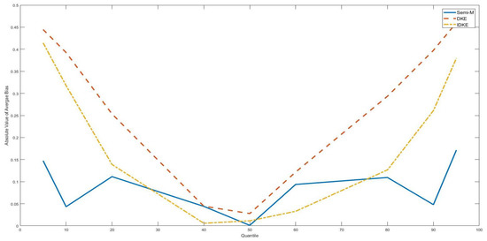
Figure 1. Average bias with ${\gamma }_0$ as various quantiles of the threshold variable, DGP 2, n = 100. This figure shows absolute values of the average bias with the true threshold level being several quantiles of the threshold variable (5th, 10th, 20th, 40th, 50th, 60th, 80th, 90th, 95th). The simulation is based on DGP 2. The sample size is 100.

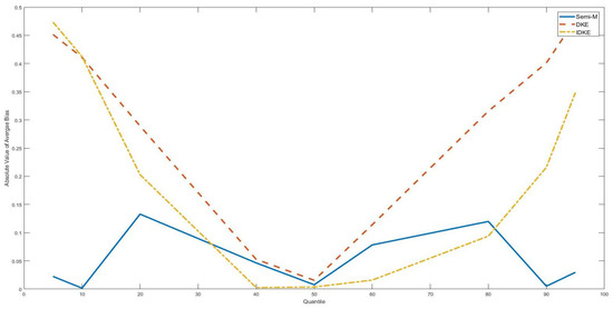
Figure 2. Average bias with ${\gamma }_0$ as various quantiles of the threshold variable, DGP 2, n = 300. This figure shows absolute values of the average bias with the true threshold level being several quantiles of the threshold variable (5th, 10th, 20th, 40th, 50th, 60th, 80th, 90th, 95th). The simulation is based on DGP 2. The sample size is 300.

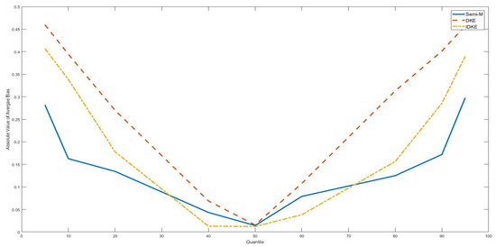
Figure 3. Average bias with ${\gamma }_0$ as various quantiles of the threshold variable, DGP 5, n = 100. This figure shows absolute values of the average bias with the true threshold level being several quantiles of the threshold variable (5th, 10th, 20th, 40th, 50th, 60th, 80th, 90th, 95th). The simulation is based on DGP 5. The sample size is 100.

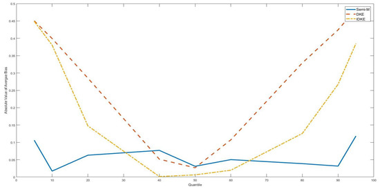
Figure 4. Average bias with ${\gamma }_0$ as various quantiles of the threshold variable, DGP 5, n = 300. This figure shows absolute values of the average bias with the true threshold level being several quantiles of the threshold variable (5th, 10th, 20th, 40th, 50th, 60th, 80th, 90th, 95th). The simulation is based on DGP 5. The sample size is 300.

6. Conclusions

In this paper, we evaluated the finite sample performance of three non-parametric threshold estimators and identified the relationship between the performances of different estimators and the position of the true threshold level with Monte Carlo methods.

The study shows, with all three estimators affected by the tail position of the true threshold value, that the semi-M estimator of Henderson et al. (2017) outperformed DKE and IDKE for roughly all DGPs considered in the paper. Interestingly, there appears to be some evidence that the distortion can be reduced if there are other covariates besides the threshold variable for the semi-M estimator and the IDKE. Consistent with the theory, we find that the realized convergence rates support the super-consistency in the threshold estimate for all three estimators. However, we find that the realized convergence rates are also affected by the position of the true threshold value. We therefore conclude that, in applied works, using the difference kernel-type estimation, researchers must be careful when the threshold estimate is at the left-tail or the right-tail of the threshold variable distribution.

References

- Afonso, Antonio, and Joao Tovar Jalles. 2013. Growth and productivity: The role of government debt. International Review of Economics and Finance 25: 384–407. [Google Scholar] [CrossRef]
- Caner, Mehmet, and Bruce Hansen. 2004. Instrumental variable estimation of a threshold model. Econometric Theory 20: 813–43. [Google Scholar] [CrossRef]
- Caner, Mehmet, Thomas J. Grennes, and Friederike N. Koehler-Geib. 2010. Finding the Tipping Point—When Sovereign Debt Turns Bad. Policy Research WP, No. 5391. New Delhi: Policy Research, pp. 1–13. [Google Scholar]
- Cecchetti, Stephen G., Madhusudan Mohanty, and Fabrizio Zampolli. 2011. The Real Effects of Debt. Working paper. Basel, Switzerland: Bank for International Settlements. [Google Scholar]
- Chan, Kung-Sik. 1993. Consistency and Limiting Distribution of the Least Squares Estimator of a Threshold Autoregressive Model. Annals of Statistics 21: 520–33. [Google Scholar] [CrossRef]
- Delgado, Miguel A., and Javier Hidalgo. 2000. Nonparametric inference on structural breaks. Journal of Econometrics 96: 113–44. [Google Scholar] [CrossRef]
- Hansen, Bruce E. 2000. Sample splitting and threshold estimation. Econometrica 68: 575–603. [Google Scholar] [CrossRef]
- Hansen, Bruce E. 2011. Threshold Autoregression in Economics. Statistics and Its Interface 4: 123–27. [Google Scholar] [CrossRef]
- Heckman, James J. 1979. Sample Selection Bias as a Specification Error. Econometrica 47: 153–61. [Google Scholar] [CrossRef]
- Henderson, Daniel J., Christopher F. Parmeter, and Liangjun Su. 2017. Nonparametric Threshold Regression: Estimation and Inference. Working paper. Singapore: Research Collection School of Economics. [Google Scholar]
- Kourtellos, Andros, Thanasis Stengos, and Chih Ming Tan. 2016. Structural Threshold Regression. Econometric Theory 32: 827–60. [Google Scholar] [CrossRef]
- Kourtellos, Andros, Thanasis Stengos, and Yiguo Sun. 2017. Endogeneity in Semiparametric Threshold Regression. Working paper. Guelph, ON, Canada: University of Cyprus and University of Guelph. [Google Scholar]
- Potter, Simon M. 1995. A Nonlinear Approach to US GNP. Journal of Applied Econometrics 10: 109–25. [Google Scholar] [CrossRef]
- Seo, Myung Hwan, and Oliver Linton. 2007. A smoothed least squares estimator for threshold regression models. Journal of Econometrics 141: 704–35. [Google Scholar] [CrossRef]
- Seo, Myung Hwan, and Yongcheol Shin. 2016. Dynamic Panels with Threshold Effect and Endogeneity. Journal of Econometrics 195: 169–86. [Google Scholar] [CrossRef]
- Yu, Ping, and Peter C. B. Phillips. 2018. Threshold Regression with Endogeneity. Journal of Econometrics 203: 50–68. [Google Scholar] [CrossRef]