1. Introduction
People who are exposed to environmental noises are affected in various ways. The most prominent effect, i.e., the effect that is experienced by the largest number of people, is annoyance, a concept that, according to Koelega [
1], is associated with
disturbance, aggravation, dissatisfaction, concern, bother, displeasure, harassment, irritation, nuisance, vexation, exasperation, discomfort, uneasiness, distress, and hate. Even with a lack of a more precise definition, annoyance is widely used to characterize the negative impact of noise. The prevalence of highly annoyed residents in a community is used as a measure to quantify the negative effects. Noise regulations are based on a percentage of the area population being highly annoyed, and the noise situation is considered unhealthy if the percentage of highly annoyed residents exceeds a specific limit. Yet there is neither any universally accepted definition of high annoyance, nor any standardized way of measuring it.
Schultz published his synthesis of social surveys on noise annoyance in 1978 [
2]. In this paper, he introduced the concept of percentage highly annoyed to quantify the prevalence of annoyance in a community. Various response scales had been used in the surveys that were reviewed. Schultz defined highly annoyed as a response corresponding to the two upper categories of a 7-point numerical scale or the three upper categories of an 11-point numerical scale. This definition represents the upper 27–29 percent of the annoyance scale. Schultz chose a relatively high degree of annoyance in order not to trivialize the annoyance concept. He wanted to include only those for which noise was a serious issue, and not just annoyed persons in general [
3]. If a verbal scale was being used, Schultz included those that indicated they were very or extremely annoyed (or using similar modifiers). This method would typically include the upper two categories of a 5-point verbal scale [
4].
Later, the US Federal Interagency Committee on Noise, FICON, declared “Annoyance is its preferred summary measure of the general adverse reaction of people to noise, and that the percentage of the area population characterized as “highly annoyed” by long-term exposure to noise is its preferred measure of annoyance” [
5]. Since then, this has become a de facto standardized way of presenting the results from social surveys on noise annoyance: the results are shown as so-called dose–response curves, also known as exposure–response functions, ERFs, showing the percentage of highly annoyed residents as a function of the noise exposure.
A lot of work has been concentrated on finding ways to describe the noise exposure in detail, either by direct measurements or predictions, but there has been little concern about the quantity percentage highly annoyed. Therefore, how annoyed, actually, is a person that is highly annoyed, and how is the degree of annoyance determined?
Accurate exposure–response functions are instrumental for regulatory purposes. Exposure limits for environmental noises are often determined on the basis of a certain percentage of the area population being highly annoyed. The European Regional Office of the World Health Organization (WHO), for instance, strongly recommends that noise should be kept below levels corresponding to 10% highly annoyed, as, according to WHO,
noise above this level is associated with adverse health effects [
6]. However, WHO makes no attempt at defining the quantity “highly annoyed”, nor does it give any advice on how the quantity should be determined.
The ISO Technical Specification ISO/TS 15666 [
7] gives a recommendation on how social or socio-acoustic surveys should be conducted, but the first version of the document did not define
highly annoyed at all. Researchers, therefore, relied on the initial ICBEN (International Commission on Biological Effects of Noise) definition [
4], which referred back to the original Schultz paper from 1978, or they used their own definition. It was only in the revised 2021 version of the ISO technical specification that a definition of highly annoyed was introduced [
7]. But, still, there are a number of variables that need to be taken into account.
The ISO technical specification 15666 introduces two different definitions of high annoyance depending on which response scales, verbal or numerical, have been used in the survey. The TS also recognizes that these two quantities are different and suggests a way of recalculating the verbal score to be comparable with the numerical score. This indirectly indicates that the numerical response scale is the preferred one, but, nevertheless, the quantity percentage highly annoyed is not uniquely defined.
Social surveys on noise annoyance are conducted by many researchers in many countries. New dose–response curves are compared, and differences are discussed with reference to previously reported data and commonly accepted reference curves. However, few researchers seem to realize that most, if not all, of the observed differences are not caused by actual changes in the basic annoyance response, but reflect differences in survey design, questionnaires, analysis methods, etc.
This paper discusses different factors that affect the results of an annoyance survey and suggests ways to compare the results from surveys that have been conducted according to different protocols.
Exposure–response curves typically show the percentage of the exposed population that is highly annoyed as a function of the equivalent noise level, or a derivative such as DNL or DENL. All factors that affect the exposure–response function, other than the accumulated noise level, are referred to as non-acoustic factors. Such factors may modify the annoyance response. This is the case, for instance, for operational changes where people who are exposed to abrupt changes typically are more annoyed. Other factors may affect the apparent results of a survey, but not necessarily the annoyance response itself. The use of different response scales, for instance, may indicate a varying prevalence of annoyance, which is only caused by methodological differences and not by differences in the actual subjective annoyance response.
2. Method
2.1. Data Collection
Data from previously reported surveys on environmental noise annoyance were collected from the literature. A database compiled by Jim Fields comprising copies of more than 1300 journal articles and reports on surveys on noise annoyance proved to be most valuable. This database covers the period 1960–2008. Data from more recent surveys was found from searches in relevant scientific journals and conference proceedings. The Socio-Acoustic Survey Data Archive (SASDA), established by the Institute of Noise Control Engineering, Japan, was also a valuable source for survey data [
8]. Some datasets were provided directly by the researchers responsible for the surveys. All the analyses were based on already completed surveys, and no new surveys were conducted or initiated.
A complete table of all the survey data would be outside the scope of this paper, but the interested reader may find comprehensive tables with relevant survey data in the following research papers:
Fidell et al.: A first-principles model for estimating the prevalence of annoyance with aircraft noise exposure [
9], (aircraft noise).
Gelderblom et al.: On the stability of community tolerance to aircraft noise [
10].
Gjestland: Recent World Health Organization regulatory recommendations not supported by existing evidence [
11], (aircraft noise).
Schomer et al.: Role of community tolerance level (CTL) in predicting the prevalence of annoyance from road and rail noise [
12].
Gjestland: On the temporal stability of people’s annoyance with road traffic noise [
13].
Fidell et al.: Updating a dosage–effect relationship for the prevalence of annoyance due to general transportation noise [
14].
Brink: A survey on exposure–response relationships for road, rail, and aircraft noise annoyance [
15].
Yokoshima et al.: Representative exposure–annoyance relationships due to transportation noises in Japan [
16].
Miedema et al.: Exposure–response relationships for transportation noise [
17].
Guski et al.: WHO environmental noise guidelines for the European region: a systematic review on environmental noise and annoyance [
18].
2.2. The CTL Method
Until recently, the favored way of developing exposure–response functions, ERFs, from annoyance survey data has been by conventional polynomial regression techniques. This method yields curves where two variables, slope and intersect, have been determined. A direct comparison of two curves with different slopes is not trivial.
There is, however, another standardized method to establish such ERFs that facilitates a comparison of different curves. This method, based on the community tolerance level (CTL), is described in the standards ISO 1996-1 [
19], and ANSI S 12.9 [
20].
The CTL method is based on the assumption that annoyance increases with the noise level at the same rate as the loudness function. This implies that all exposure–response functions have the same “shape”, and the only variable is the positioning of the exposure–response curve relative to the noise axis (x-axis). Therefore, as opposed to standard polynomial regression where the objective is to find a function that has “the best fit” to a set of data points, the CTL method seeks to position a fixed function to these data points. The position is described by the noise level at which 50% of the exposed residents are highly annoyed (and the other half not highly annoyed). This is the so-called community tolerance level, CTL or Lct. A high CTL value characterizes a community that is very tolerant to noise, and, hence, the annoyance with noise is low, and a low CTL value indicates the opposite, low tolerance to noise and a high prevalence of annoyance.
The exposure–response function, i.e., the probability of being highly annoyed at a certain noise level, is given by the following equation:
where the exponent
a is given by: (
)
0.3The complete exposure–response function is uniquely described by a single decibel quantity Lct. This quantity shifts the position of the ERF back and forth along the noise axis. The difference in the annoyance response between two noise situations can, therefore, be described with a single number, the difference between the CTL values. This quantity can be explained as the number of decibels the noise in one situation must be changed in order to get the same annoyance response as in the other situation.
If community A is characterized by Lct = 74 dB and community B by Lct = 78 dB, one may argue that residents of community B on average will tolerate 4 dB higher noise levels in order to express the same degree of annoyance as residents of community A.
2.3. Data Analyses
New exposure–response functions based on the CTL method for all the selected surveys were established on the basis of reported paired observations of noise exposure and prevalence of high annoyance. For some surveys, we had access to the original individual responses, but, in most cases, we had to rely on pooled data: prevalence of high annoyance per exposure bin, typically 5 dB wide.
The surveys were then sorted and analyzed based on different criteria such as wording of the questionnaire, presentation mode, response scales, principal noise source, etc. This was carried out by the author together with other colleagues. Some of the results from these analyses have been published as separate papers elsewhere [
9,
10,
12,
13,
21,
22]. This paper summarizes the results and compiles them in a way that renders them suitable for direct application when the task is to compare results from social surveys on noise annoyance that have been conducted in different ways and according to different protocols.
3. Non-Acoustic Factors
3.1. Response Scales
The technical specification ISO/TS 15 666 recommends two standardized questions to be included in a survey [
7]. Both deal with the assessment of long-term noise annoyance for a specified period of time (e.g., 12 months). One question refers to a 5-point verbal response scale and the other to an 11-point numerical scale. Highly annoyed is defined by the two upper categories of the verbal scale and the three upper categories of the numerical scale. The document underlines that these two definitions of highly annoyed do not yield identical answers. When reporting survey results, it is, therefore, necessary to specify how the quantity highly annoyed was derived; HA
V for the verbal scale and HA
N for the numerical scale. HA
V is normally larger. The technical specification also has a procedure for transforming HA
V to a quantity, HA
VW (highly annoyed, weighted verbal response), that can be readily compared with the numerical response.
Gjestland and Morinaga have shown that the average difference between the two quantities is equivalent to a 6 dB shift in the noise exposure [
22]. They analyzed 43 annoyance surveys on transportation noise, aircraft, rail, and road traffic, comprising nearly 27,000 respondents in which the participants were asked to assess the noise situation using both a numerical and a verbal scale as recommended by ICBEN [
4]. These surveys had been conducted in Germany, Japan, Norway, Switzerland, and Vietnam. References to all the original response data for these 43 surveys can be found in Gjestland and Morinaga [
22].
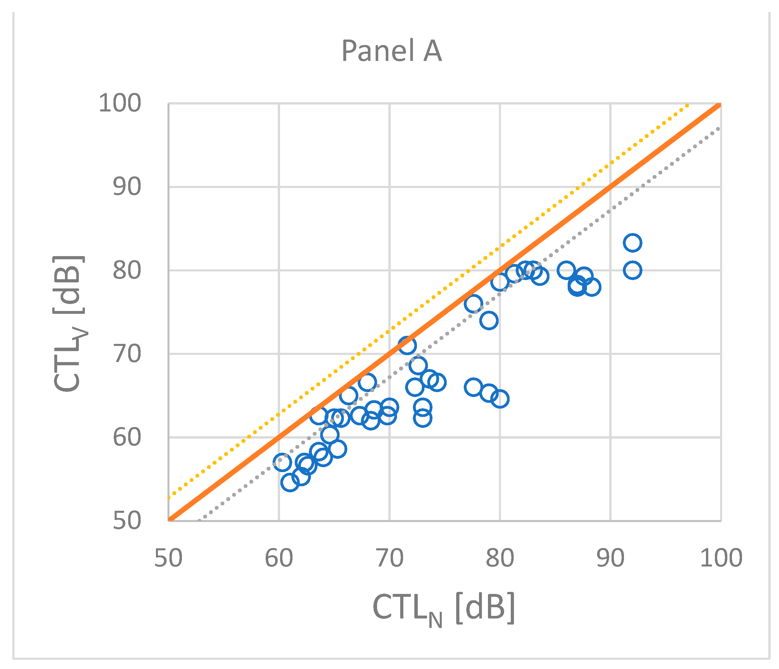
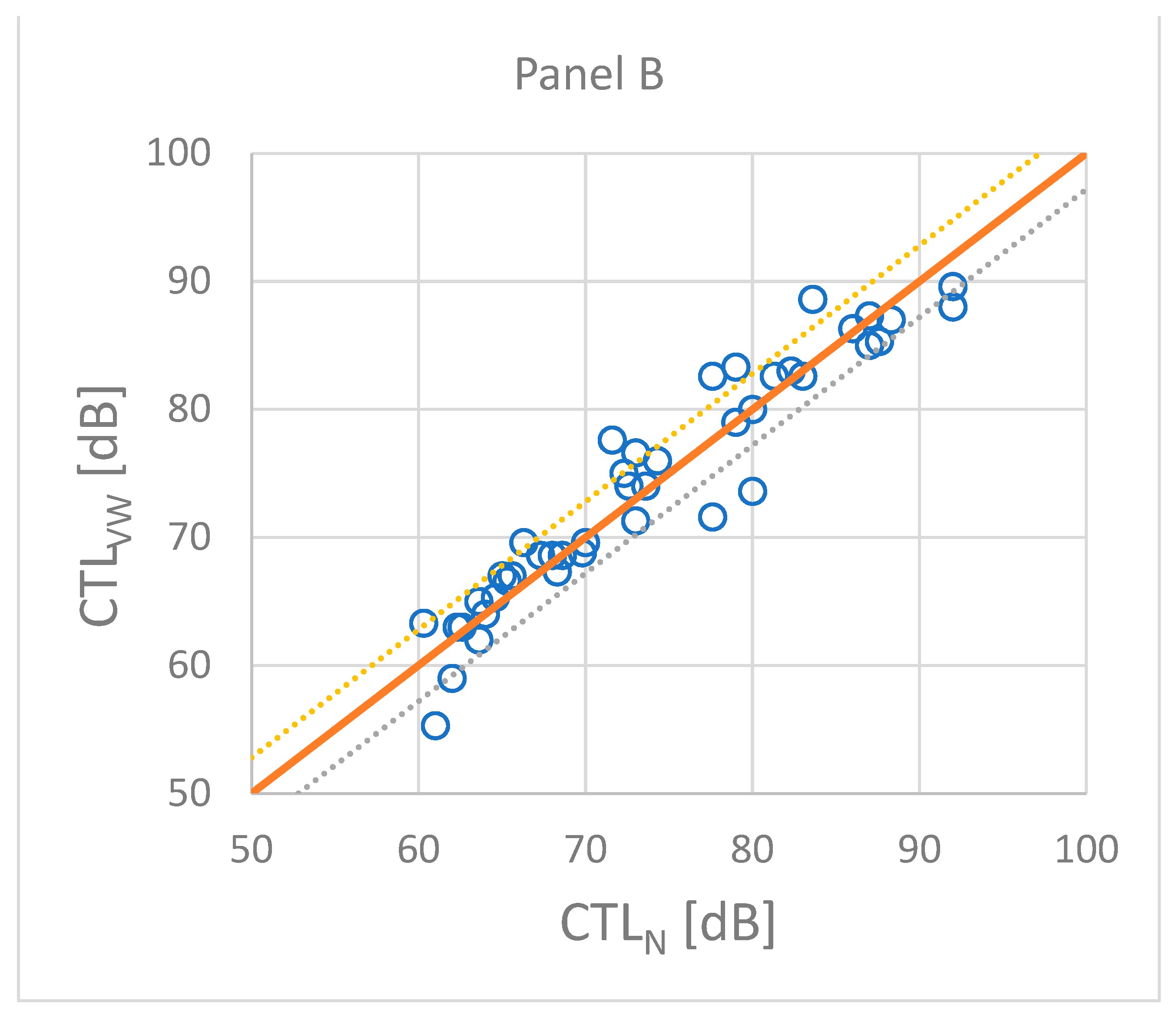
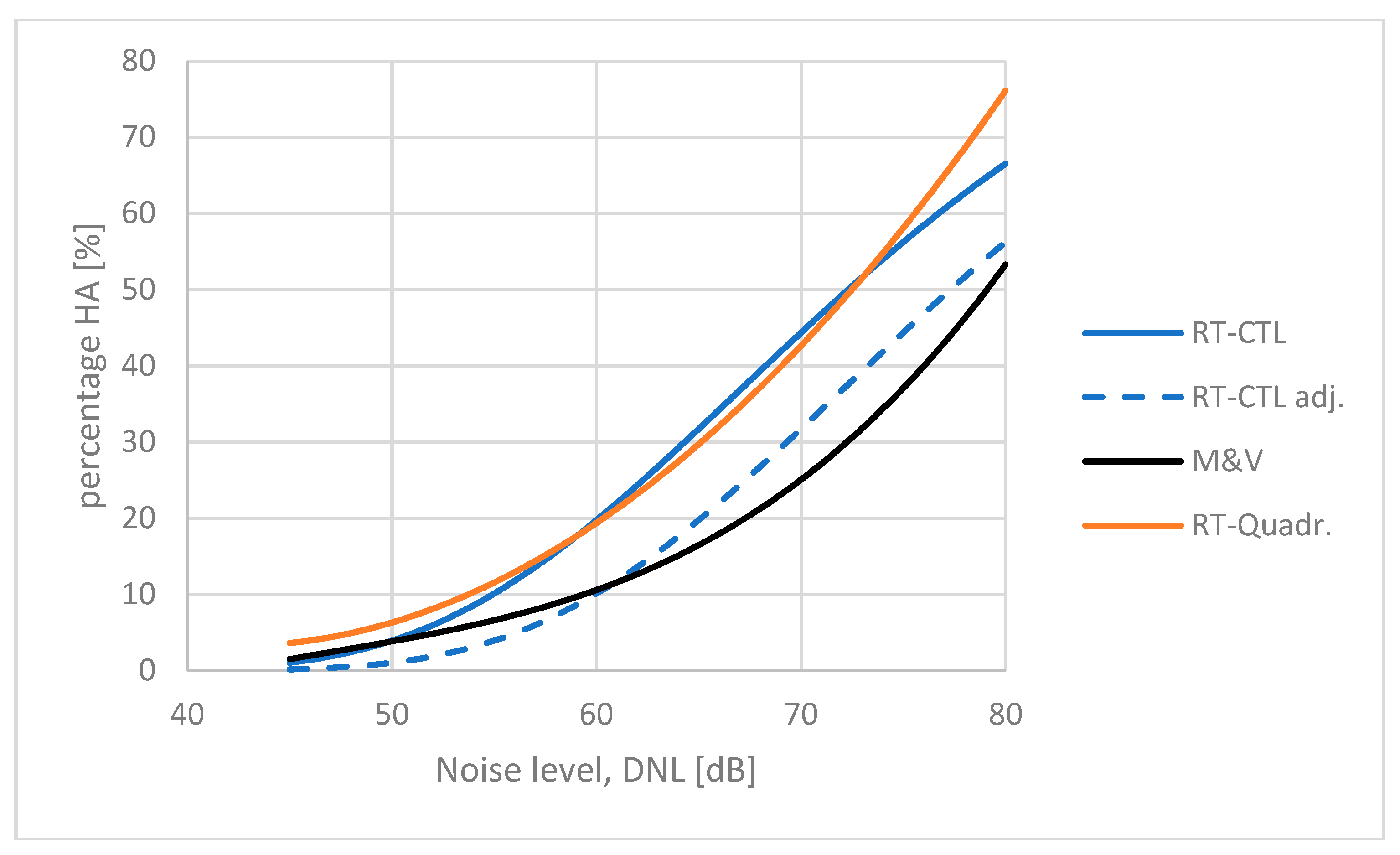
Figure 1 illustrates the effect of making adjustments to the annoyance assessed on the verbal scale. The CTL value based on the numerical scale is normally larger than the CTL value for the verbal scale as shown in panel A (a high CTL value means low annoyance). After an adjustment, the CTL values are brought within a difference of typically less than ±2 dB as shown in panel B.
Since the annoyance assessments in these surveys were carried out by the same individuals and the only outcome of the analysis was the relative difference between the two responses, any possible confounding factors become irrelevant. Gjestland and Morinaga [
22] found that people who were classified as highly annoyed according to their verbal responses seemed to tolerate, on average, 6 dB higher noise levels in order for their numerical responses to indicate the same degree of high annoyance.
3.2. Mode of Presentation
The earliest surveys were usually conducted as face-to-face interviews in the respondent’s home. Later on, telephone interviews became a favorite method, being faster and less expensive to carry out. Postal surveys are also being used. The potential respondents are contacted by mail or otherwise, and are requested to complete a self-administered written questionnaire, which, in turn, is returned by mail. In some countries, this has become the favored survey method as there is an increasing number of potential respondents that decline to participate in telephone surveys.
The US Federal Aviation Administration recently conducted a large survey by mail [
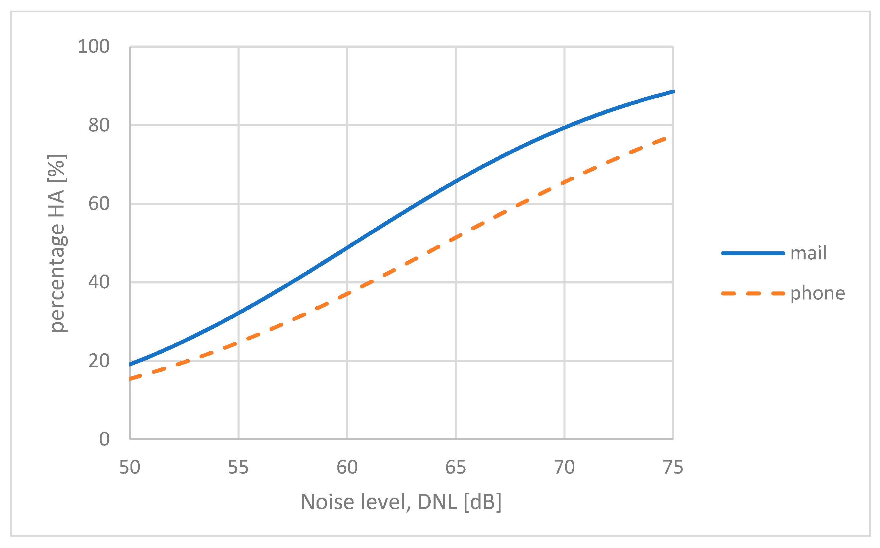
23], but the researchers that were responsible for the survey also complemented the study with a smaller number of telephone interviews with the same mail respondents to check the influence of the survey mode. The participants in these studies, via mail or via telephone, were selected randomly using the same selection protocol. A total of 10,000 individual responses were collected via mail and about 2000 responses via phone interviews. Miller et al. who conducted the survey [
23] found that people responding to the written questionnaire, on average, seemed to be more annoyed than people responding to the telephone interview. They found that the difference increased with increasing noise exposure levels. The average difference across the range 50 dB <
Ldn < 75 dB was equivalent to a shift in the exposure of about 5 dB. The results reported by Miller et al. are shown in
Figure 2. The two curves represent a logistic fit to the responses from the mail survey and phone survey respectively.
A CTL analysis of the two response categories using data reported in [
23] confirmed this finding, the difference in CTL values being 4.8 dB.
The issue of the survey mode is an ongoing discussion. It has, for a long time, been recognized that the response to a survey question may depend on how the question is presented: one-on-one interview, postal or web-based questionnaire, etc.—see, inter alia, Brink [
24], Canturia et al. [
25], and National Academies of Sciences [
26]. The results presented by Miller et al. [
23] quantify such differences.
Fidell et al. have analyzed 45 surveys on aircraft noise conducted either face-to-face, via telephone, or as a postal survey [
27]. They found no significant differences between face-to-face and telephone interviews, both involving contact with a live agent. However, mail surveys produced a higher prevalence of highly annoyed respondents with an average difference equivalent to a 10 dB shift in the noise exposure. This difference may also be due to the combined effect of other non-acoustic factors, but the result shows the same tendency as observed by Miller et al. [
23]. More survey results that allow a direct comparison of the two survey modes—interview by a live agent or a self-reporting written questionnaire—as reported by Miller et al. have not been found. Based on the other analyses reported above, however, we find it plausible that the difference between the two modes corresponds to a shift in the noise level of at least 5 dB, and people dealing with a live survey agent report lower annoyance.
3.3. Changes in Airport Operations
The effect of abrupt changes in the airport operations has been observed in many aircraft noise studies. Most airports experience a gradual increase in traffic over the years. In most cases, this growth is small, and week-to-week or year-to-year changes in the noise exposure will hardly be noticed by the neighborhood community. However, occasionally, abrupt changes will occur such as the opening of a new runway, the introduction of a new fleet of aircraft (for instance, if a major airline is moving to a new hub), the introduction of new operational procedures and new flight trajectories, etc.
Janssen and Guski [
28] have presented a study on temporal trends in the aircraft noise annoyance response. They analyzed a set of 32 aircraft noise studies contained in the TNO database. They observed that abrupt changes in the airport operations will affect the annoyance response, and, therefore, introduced a classification procedure as follows:
We call airports “low-rate change airports” (LRC), as long as there is no indication of a sustained abrupt change of aircraft movements, or the published intention of the airport to change the number of movements within 3 years before and after the study. An abrupt change is defined here as a significant deviation in the trend of aircraft movements from the trend typical for the airport. Each trend is calculated by means of total movement data during a five-year period. If the typical trend is disrupted significantly and permanent, we call this a “high-rate change airport” (HRC). We also classify an airport in the latter category if there has been widespread public discussion about operational plans within 3 years before and after the study.
Janssen and Guski found that the average difference in the annoyance response between an HRC and an LRC airport was equal to a 6 dB shift in the exposure level.
Gelderblom et al. [
10] have made a similar analysis of a set of 62 aircraft noise annoyance surveys to study the stability of community tolerance to noise. Their dataset comprised about 650 paired observations of aircraft noise exposure and the prevalence of high annoyance. Gelderblom et al. carried out a classification of the airports according to the protocol suggested by Janssen and Guski and defined 45 LRC airports and 17 HRC airports. They found that the average difference in the annoyance response between these two categories of airports was equal to a 9 dB shift in noise exposure. People living near a high-rate change airport seem to tolerate 9 dB less noise in order to express the same degree of annoyance as residents living in a low-rate change airport community.
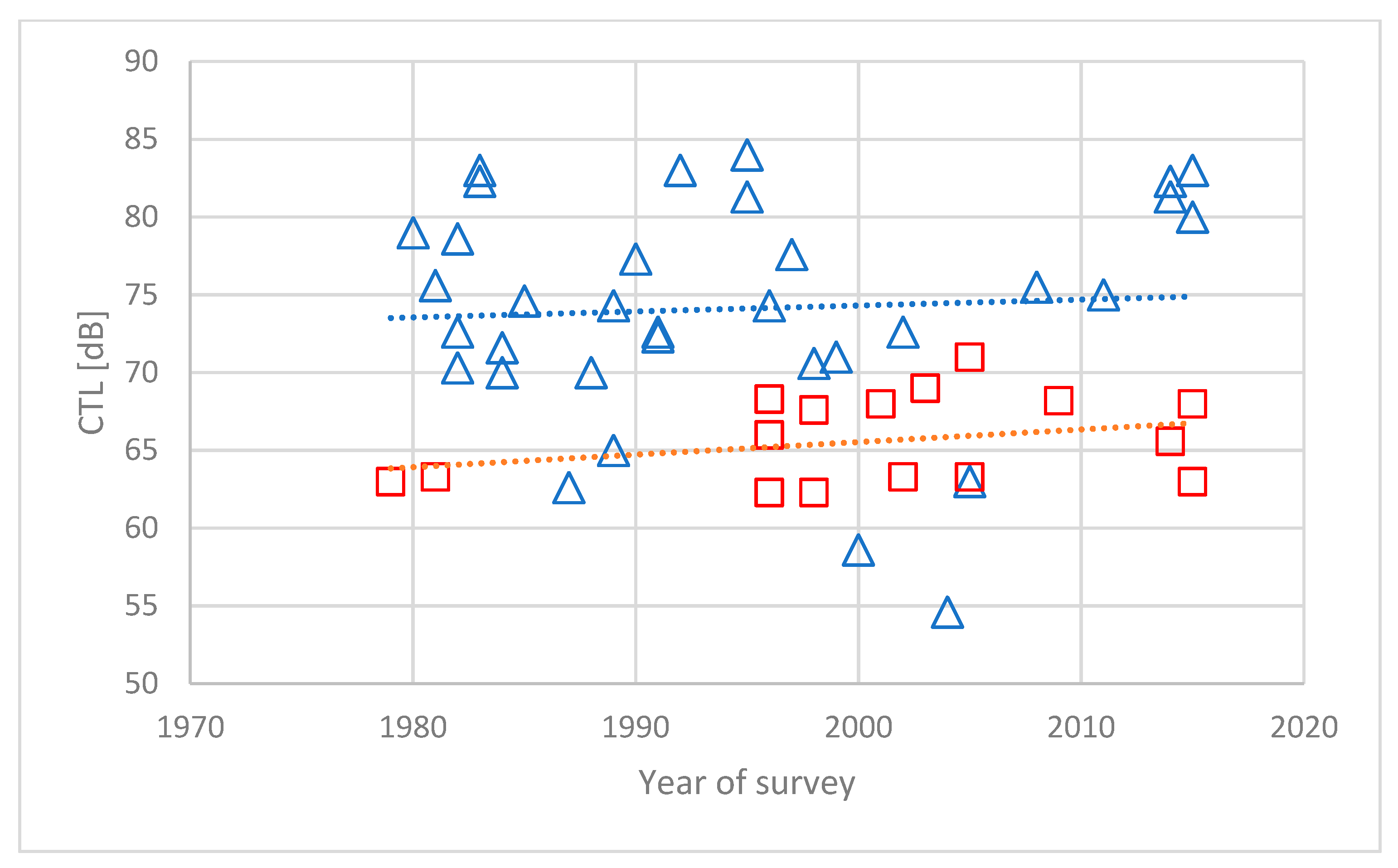
The results reported by Gelderblom et al. [
10] are shown in
Figure 3. The figure shows CTL values for aircraft noise surveys conducted over a period of about 35 years. The airports have been classified as LRC (blue triangles) or HRC (red squares) according to the proposed method by Janssen and Guski. Trendlines have been fitted to the two datasets. Both trendlines have a small positive slope, indicating that the CTL values increase a little for more recent studies. This indicates a decrease in the annoyance response, contrary to the claim by several authors [
18,
29]. The average difference between the two lines is about 9 dB.
The increased prevalence of annoyance due to a situation that makes the airport an HRC airport actually seems to last longer than the three-year period suggested by Janssen and Guski. This is discussed by Gelderblom et al. [
10]. They argue that the shift in a person’s attitude may be permanent, and that the community response only shifts gradually as people move in and out of the airport neighborhood.
Many new noise surveys are conducted because noise has become an issue of public debate, and the residents demand proof of the actual annoyance situation. Since surveys are time-consuming and expensive to carry out, it is more likely than not that new study sites are located at an HRC airport rather than at an LRC airport. A greater portion of HRC airports in the total number of noise surveys may explain the claim that aircraft noise annoyance is increasing [
30]. For most of the airports characterized as HRC in this study, the classification was based on quite recent operational changes or recent announcements of controversial plans.
We find it plausible that a similar increase in the annoyance response due to abrupt changes may also be observed for other noise sources, for instance, in connection with the construction of a new road or a major refurbishing of an existing one.
3.4. Traffic Volume
Annoyance with transportation noise increases when the traffic volume increases. An increased number of noise events per day will increase the DNL level. However, the annoyance seems to increase at a faster rate than the equivalent level.
Gjestland et al. [
21] have studied the prevalence of noise-induced annoyance and its dependency on the number of aircraft movements. They analyzed the results from 32 aircraft noise surveys and concluded that, for a given noise exposure level, the percentage of highly annoyed residents increased equivalent to a DNL increase of 1.8 dB per doubling (= 6 × log(2)) of the number of aircraft movements. This increase comes in addition to the regular 3 dB per doubling.
Consequently, residents living near a small airport seem to tolerate 6 dB more noise than neighbors to an airport with ten times more traffic (= 6 × log(10)) in order to express the same degree of annoyance.
A similar analysis of road traffic noise surveys shows the same tendency, but with a slightly smaller effect: 1.5 dB per doubling (= 5 × log(2)) [
31].
4. Reference Curves
The exposure–response curves for transportation noise sources developed by Miedema and Vos [
17] are widely used as standard references. These so-called Miedema curves are simple second-order polynomial regression functions fitted to the results of a selection of surveys. The curves were refined by Miedema and Oudshoorn [
32] who used a third-order regression function. The Miedema curve for aircraft noise is almost identical to a CTL function anchored at
Lct = 73.3 dB. An analysis of the input data used by Miedema and Vos when they derived at this average ERF for aircraft noise shows that the curve can be used to predict the dose–response function for an airport with about 250,000 aircraft movements per year. For airports with other traffic volumes, the curve should be adjusted according to paragraph 2.7.
Schomer et al. [
12] have shown that a CTL function anchored at
Lct = 78.3 dB is a good approximation for the Miedema curve for road traffic noise. This curve seems to fit a situation with a traffic volume of about 2000 ADT (annual daily traffic) [
31].
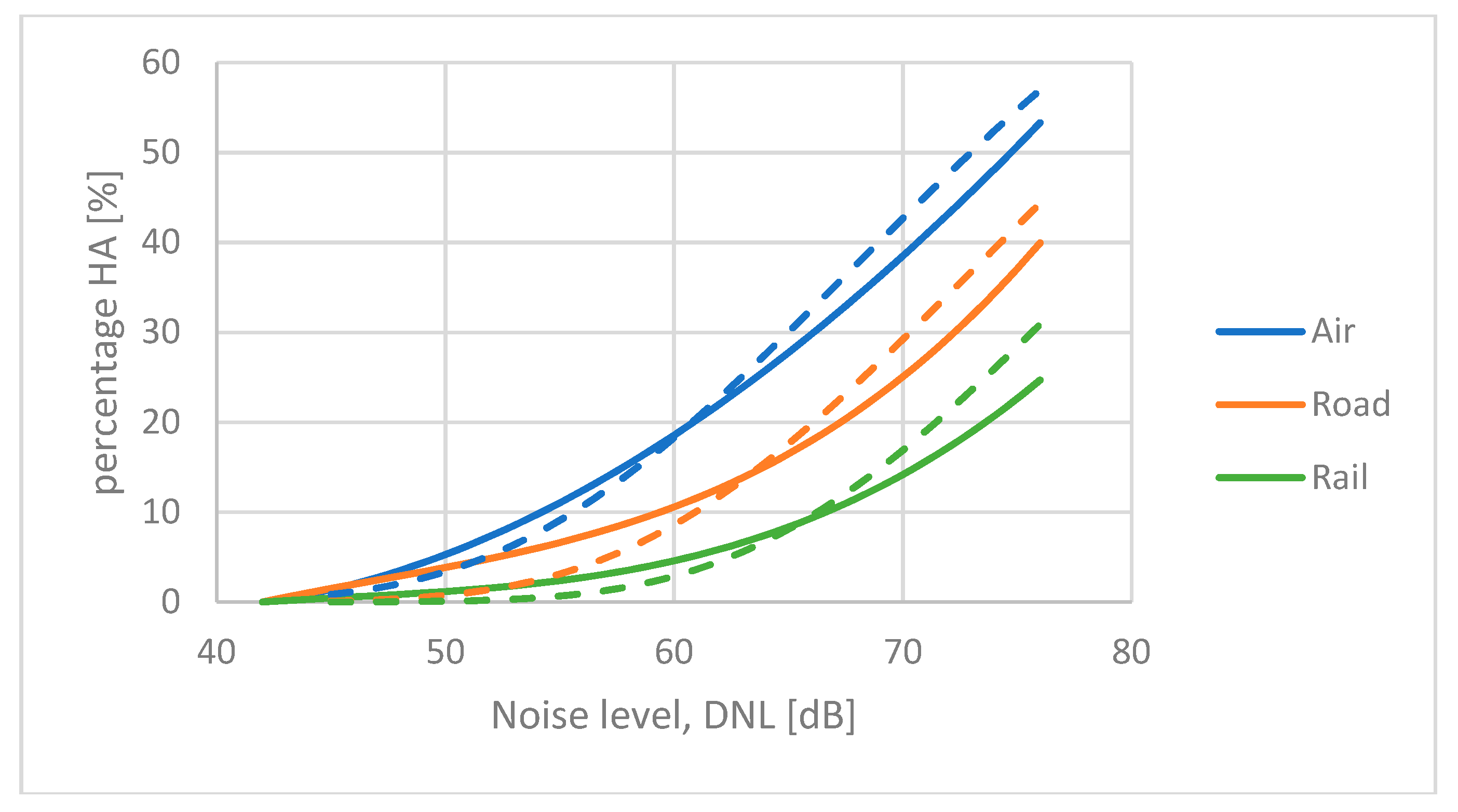
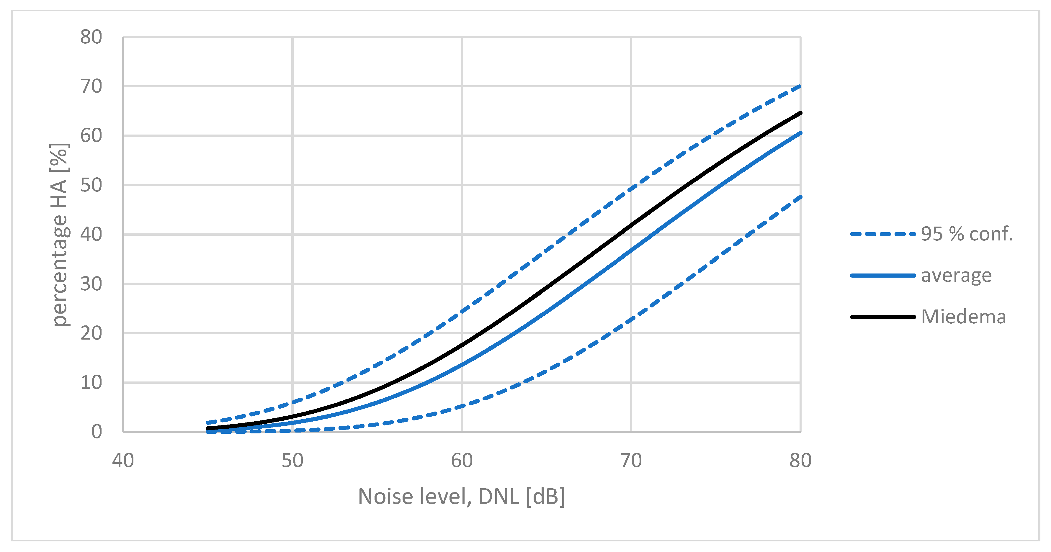
Figure 4 shows the Miedema curves for air, road, and rail traffic (solid lines), together with the CTL curves (dashed lines) that are fitted to similar datasets.
The difference between the Midema curves and the CTL functions seem to increase towards higher noise levels. This is mainly due to the fact that the Miedema curves are polynomial regression functions, and the CTL curves are logistic functions.
The Miedema curves for transportation noise are based on surveys conducted between 1965 and 1994. They can still be considered valid according to the findings by Gelderblom et al.


