
Estimating Inhalation Exposure Resulting from Evaporation of Volatile Multicomponent Mixtures Using Different Modelling Approaches

Abstract
:1. Introduction
2. Materials and Methods
2.1. Estimating Evaporation Rates of Liquid Mixtures
2.2. Well-Mixed Room Model for Instantaneous Application (WMR_inst)
2.3. Near-Field/Far-Field Model for Instantaneous Application (NF/FF_inst)
2.4. Well-Mixed Room Model for Continuous Application (WMR_cont)
2.5. Near-Field/Far-Field Models for Continuous Application (NF/FF_cont and NF/FF_mov)
3. Results
4. Discussion
5. Conclusions
Author Contributions
Funding
Conflicts of Interest
Appendix A
Appendix A.1. Pseudocode for the WMR_cont Scenario Using the Extended Euler Method
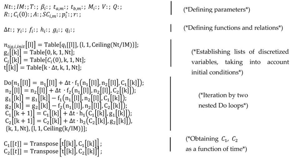
Appendix A.2. Pseudocode for Continuous Application of a Binary Mixture in a Moving Near-Field Scenario Using Euler’s Method

References
- Delmaar, J.E.; Park, M.V.D.Z.; van Engelen, J.G.M. ConsExpo 4.0 Consumer Exposure and Uptake Models Program Manual, RIVM Report 320104004/2005; RIVM: De Bilt, The Netherlands, 2006.
- Advanced REACH Tool. ART. 2013. Available online: https://www.advancedREACHtool.com/ (accessed on 17 August 2021).
- European Parliament and the Council [EP]. Regulation (EU) No 528/2012 of the European Parliament and of the Council of 22 May 2012 Concerning the Making Available on the Market and Use of Biocidal Products; European Parliament and the Council: Strasbourg, France, 2012. [Google Scholar]
- European Parliament and the Council [EP]. Regulation (EU) No 1907/2006 of the European Parliament and of the Council of 18 December 2006 Concerning the Registration, Evaluation, Authorisation and Restriction of Chemicals (REACH); European Parliament and the Council: Strasbourg, France, 2006. [Google Scholar]
- European Chemicals Agency. Recommendation No. 16, BPC Ad hoc Working Group on Human Exposure, Applicability of ConsExpo for Water Based Disinfectants; ECHA: Helsinki, Finnland, 2019.
- Abattan, S.F.; Lavoue, J.; Halle, S.; Bahloul Ali Drolet, D. Modeling occupational exposure to solvent vapors using the Two-Zone (near-field/far-field) model: A literature review. J. Occup. Environ. Hyg. 2021, 18, 51–64. [Google Scholar] [CrossRef] [PubMed]
- Arnold, S.F.; Shao, Y.; Ramachandran, G. Evaluation of the well mixed room and near-field far-field models in occupational settings. J. Occup. Environ. Hyg. 2017, 9, 694–702. [Google Scholar] [CrossRef] [PubMed]
- Lennert, A.; Nielsen, F.; Breum, N.O. Evaluation of Evaporation and Concentration Distribution Models in a Test Chamber Study. Ann. Occup. Hyg. 1997, 41, 625–641. [Google Scholar] [PubMed]
- Gmehling, J.; Weidlich, U.; Lehmann, E.; Fröhlich, N. Verfahren zur Berechnung von Luftkonzentrationen bei Freisetzung von Stoffen aus flüssigen Produktgemischen (Teil 1). Staub-Reinhalt. Der Luft 1989, 49, 227–230. [Google Scholar]
- Weidlich, U.; Gmehling, J. Expositionsabschätzung–Ein Methodenvergleich Mit Hinweisen für Die Praktische Anwendung; Schriftenreihe der Bundesanstalt für Arbeitsschutz, Fb 488: Dortmund, Germany, 1986. [Google Scholar]
- McCready, D.; Fontaine, D. Refining ConsExpo Evaporation and Human Exposure Calculations for REACH. Hum. Ecol. Risk Assess. 2010, 16, 783–800. [Google Scholar] [CrossRef]
- Nielsen, F.; Olsen, E.; Fredenslund, F. Prediction of isothermal evaporation rates of pure volatile organic compounds in occupational environments—A theoretical approach based on laminar boundary layer theory. Ann. Occup. Hyg. 1995, 39, 497–511. [Google Scholar]
- Fredenslund, A.; Jones, R.L.; Prausnitz, J.M. Group-Contribution Estimation of Activity Coefficients in Nonideal Liquid Mixtures. AIChE J. 1975, 21, 1086–1099. [Google Scholar] [CrossRef]
- Gmehling, J. Group contribution methods for the estimation of activity coefficients. Fluid Phase Equilibria 1986, 30, 119–134. [Google Scholar] [CrossRef]
- Zuend, A. Modelling the Thermodynamics of Mixed Organic-Inorganic Aerosols to Predict Water Activities and Phase Separations. Ph.D. Thesis, ETH Zurich, Zurich, Switzerland, 2007. Available online: http://e-collection.ethbib.ethz.ch/view/eth:30457 (accessed on 17 August 2021). [CrossRef]
- Zuend, A.; Marcolli, C.; Booth, A.M.; Lienhard, D.M.; Soonsin, V.; Krieger, U.K.; Topping, D.O.; McFiggans, G.; Peter, T.; Seinfeld, J.H. New and extended parameterization of the thermodynamic model AIOMFAC: Calculation of activity coefficients for organic-inorganic mixtures containing carboxyl, hydroxyl, carbonyl, ether, ester, alkenyl, alkyl, and aromatic functional groups. Atmos. Chem. Phys. 2011, 11, 9155–9206. [Google Scholar]
- Zuend, A.; Marcolli, C.; Luo, B.P.; Peter, T. A thermodynamic model of mixed organic-inorganic aerosols to predict activity coefficients. Atmos. Chem. Phys. 2008, 8, 4559–4593. [Google Scholar] [CrossRef]
- Zuend, A.; Marcolli, C.; Peter, T.; Seinfeld, J.H. Computation of liquid-liquid equilibria and phase stabilities: Implications for RH-dependent gas/particle partitioning of organic-inorganic aerosols. Atmos. Chem. Phys. 2010, 10, 7795–7820. [Google Scholar] [CrossRef]
- Margules, M. Über die Zusammensetzung der gesättigten Dämpfe von Misschungen. In Sitzungsberichte der Kaiserliche Akadamie der Wissenschaften Wien Mathematisch-Naturwissenschaftliche Klasse I; Kaiserliche Akadamie der Wissenschaften: Vienna, Austria, 1895; Volume 104, pp. 1243–1278. [Google Scholar]
- van Laar, J.J. Über Dampfspannungen von binären Gemischen (The vapor pressure of binary mixtures). Z. Physik. Chem. 1910, 72, 723–751. [Google Scholar] [CrossRef]
- Wilson, G.M. Vapor-liquid equilibrium. XI. A new expression for the excess free energy of mixing. J. Am. Chem. Soc. 1964, 86, 127–130. [Google Scholar] [CrossRef]
- Renon, H.; Prausnitz, J.M. Local compositions in thermodynamic excess functions for liquid mixtures. AIChE J. 1968, 14, 135–144. [Google Scholar] [CrossRef]
- Abrams, D.S.; Prausnitz, J.M. Statistical thermodynamics of liquid mixtures: A new expression for the excess Gibbs energy of partly or completely miscible systems. AIChE J. 1975, 21, 116–128. [Google Scholar] [CrossRef]
- Heinsohn, R.J. General Ventilation Well-Mixed Mode (Chapter 5). In Industrial Ventilation Engineering Principles; John Wiley & Sons, Inc.: New York, NY, USA, 1991. [Google Scholar]
- Wolfram Research, Inc. Mathematica, Version 12.1; Wolfram Research: Champaign, IL, USA, 2020. [Google Scholar]
- Dahmen, W.; Reusken, A. Numerik für Ingenieure und Naturwissenschaftler; Springer: Berlin/Heidelberg, Germany, 2006. [Google Scholar]
- Cherrie, J.W.; Schneider, T. Validation of a new method for structured subjective assessment of past concentrations. Ann. Occup. Hyg. 1999, 43, 235–245. [Google Scholar] [CrossRef]
- Cherrie, J.W. The effect of room size and general ventilation on the relationship between near- and far-field concentrations. Appl. Occup. Environ. Hyg. 1999, 14, 539–546. [Google Scholar] [CrossRef]
- Kulmala, I. Calculation of Vertical Buoyant Plumes. In I: Proceedings of Ventilation ‘97 Global Developments in Industrial Ventilation; Goodfellow, H., Tahti, E., Eds.; Canadian Environment Industry Association: Ottawa, ON, Canada, 1997; pp. 393–398. [Google Scholar]
- Evans, W.C. Development of continuous-application source terms and analytical solutions for one- and two-compartment systems. In Characterising Sources of Indoor Air Pollution and Related Sink Effects; ASTM STP 1287; Tichenor, B.A., Ed.; American Society for Testing and Materials: Philadelphia, PA, USA, 1996; pp. 279–293. [Google Scholar]
- Zemansky, M.W.; Dittman, R.H. Heat and Thermodynamics; McGraw Hill: New York, NY, USA, 1984. [Google Scholar]
- Thibodeaux, L.J. Exchange rates between air and water. In Chemodynamics; Wiley-Interscience: New York, NY, USA, 1979. [Google Scholar]
- Handbook of Chemistry and Physics, 59th ed.; CRC Press: Boca Raton, FL, USA, 1979.
- Olson, J.D. The vapor pressure of pure and aqueous glutaraldehyde. Fluid Phase Equilibria 1998, 150, 713–720. [Google Scholar] [CrossRef]
- Schumb, W.C.; Satterfield, C.N.; Wentworth, R.L. Report No. 43, Hydrogen Peroxide Part Two; Massachusetts Institute of Technology, Division of Industrial Cooperation Project 6552: Cambridge, MA, USA, 1953. [Google Scholar]
- Perry, R.H.; Chilton, C.H. (Eds.) Chemical Engineer’s Handbook; McGraw-Hill: New York, NY, USA, 1973; pp. 233–234. [Google Scholar]
- Matthies, H.G. Quantifying uncertainty: Modern computational representation of probability and applications. In Extreme Man-made and Natural Hazards in Dynamics of Structures; Springer: Berlin/Heidelberg, Germany, 2007; pp. 105–135. [Google Scholar]
- WHO. Uncertainty and Data Quality in Exposure Assessment [Part 1: Guidance Document on Characterizing and Communicating Uncertainty in Exposure Assessment. Part 2: Hallmarks of Data Quality in Chemical Exposure Assessment]; WHO: Geneva, Switzerland, 2008. [Google Scholar]
- Hofstetter, E.; Spencer, J.W.; Hiteshew, K.; Coutu, M.; Nealley, M. Evaluation of recommended REACH exposure modeling tools and near-field, far-field model in assessing occupational exposure to toluene from spray paint. Ann. Occup. Hyg. 2013, 57, 210–220. [Google Scholar]
- Jayjock, M.A.; Armstrong, T.; Taylor, M. The Daubert standard as applied to exposure assessment modeling using the two-zone (NF/FF) model estimation of indoor air breathing zone concentration as an example. J. Occup. Environ. Hyg. 2011, 8, D114–D122. [Google Scholar] [CrossRef]
- Keil, C.B.; Nicas, M. Predicting room vapor concentrations due to spills of organic solvents. AIHA J. 2003, 64, 445–454. [Google Scholar] [CrossRef]
- Spencer, J.W.; Plisko, M.J.; Occup, J. A Comparison Study Using a Mathematical Model and Actual Exposure Monitoring for Estimating Solvent Exposures During the Disassembly of Metal Parts. Environ. Hyg. 2007, 4, 253–259. [Google Scholar] [CrossRef]
- Nicas, M.; Neuhaus, J. Predicting Benzene Vapor Concentrations with a Near Field/Far Field Model. J. Occup. Environ. Hyg. 2008, 5, 599–608. [Google Scholar] [CrossRef]
- Zhang, Y.; Banerjee, S.; Yang, R.; Lungu, C.; Ramachandran, G. Bayesian Modeling of Exposure and Airflow Using Two-Zone Models. Ann. Occup. Hyg. 2009, 53, 409–424. [Google Scholar] [PubMed]
- Keil, C.B.; Simmons, C.E.; Anthony, T. Mathematical Models for Estimating Occupational Exposure to Chemicals, 2nd ed.; American Industrial Hygiene Association: Fairfax, VA, USA, 2009. [Google Scholar]
- Ganser, G.H.; Hewett, P. Models for nearly every occasion: Part II—Two box models. J. Occup. Environ. Hyg. 2017, 14, 58–71. [Google Scholar] [CrossRef]
- Hewett, P.; Ganser, G.H. Models for nearly every occasion: Part I—One box models. J. Occup. Environ. Hyg. 2017, 14, 49–57. [Google Scholar] [CrossRef] [PubMed]


| Indices: | |
|---|---|
| i | counting index for particular substances |
| l | counting index for particular area elements |
| k | counting index for particular time steps |
| m | counting index for the application cycle |
| room | parameters referring to the air space in the room in case of well-mixed-room models |
| nf | parameters referring to the air space in the near field in case of two-box models |
| ff | parameters referring to the air space in the far field in case of two-box models |
| nf/ff | used to indicate an air exchange rate between near and far field |
| vent | parameters referring the air exchanged by ventilation |
| liq | parameters referring to the liquid layer |
| air | parameters referring to air |
| evap | parameters indicating an evaporating fraction |
| A | parameters referring to the entire treated surface |
| ΔA | parameters referring to a fraction of the treated area (“area element”) |
| app | refers to the application duration |
| expo | refers to the total simulated exposure duration |
| init | initial value (for product amounts applied or air concentrations) |
| a | refers to starting time of application cycle |
| b | refers to end time of application cycle |
| P | refers to the entire product |
| Parameters and units: | |
| p: | vapour pressure [Pa] |
| p*: | vapour pressure of a pure substance [Pa] |
| x: | molar fraction |
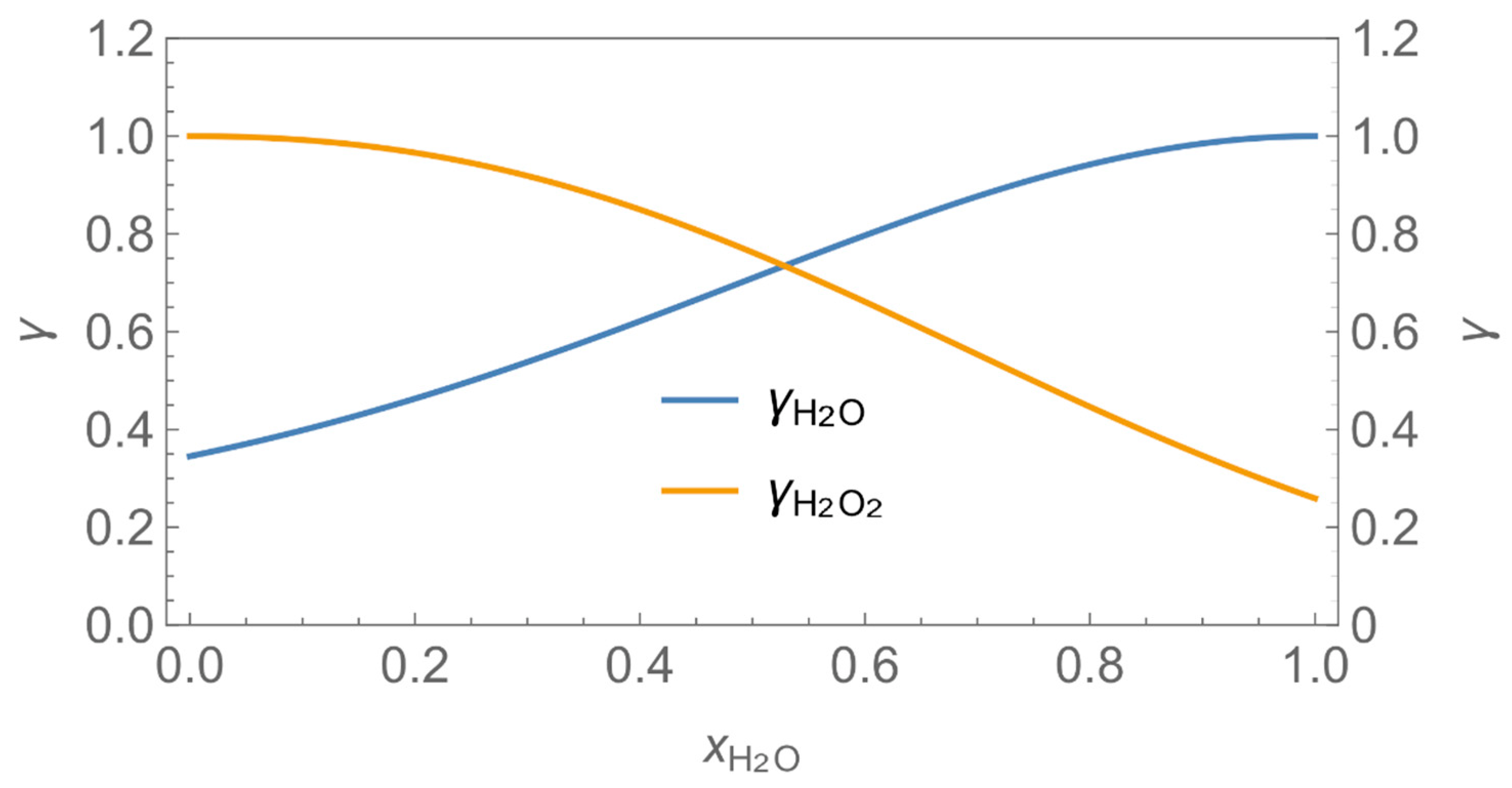
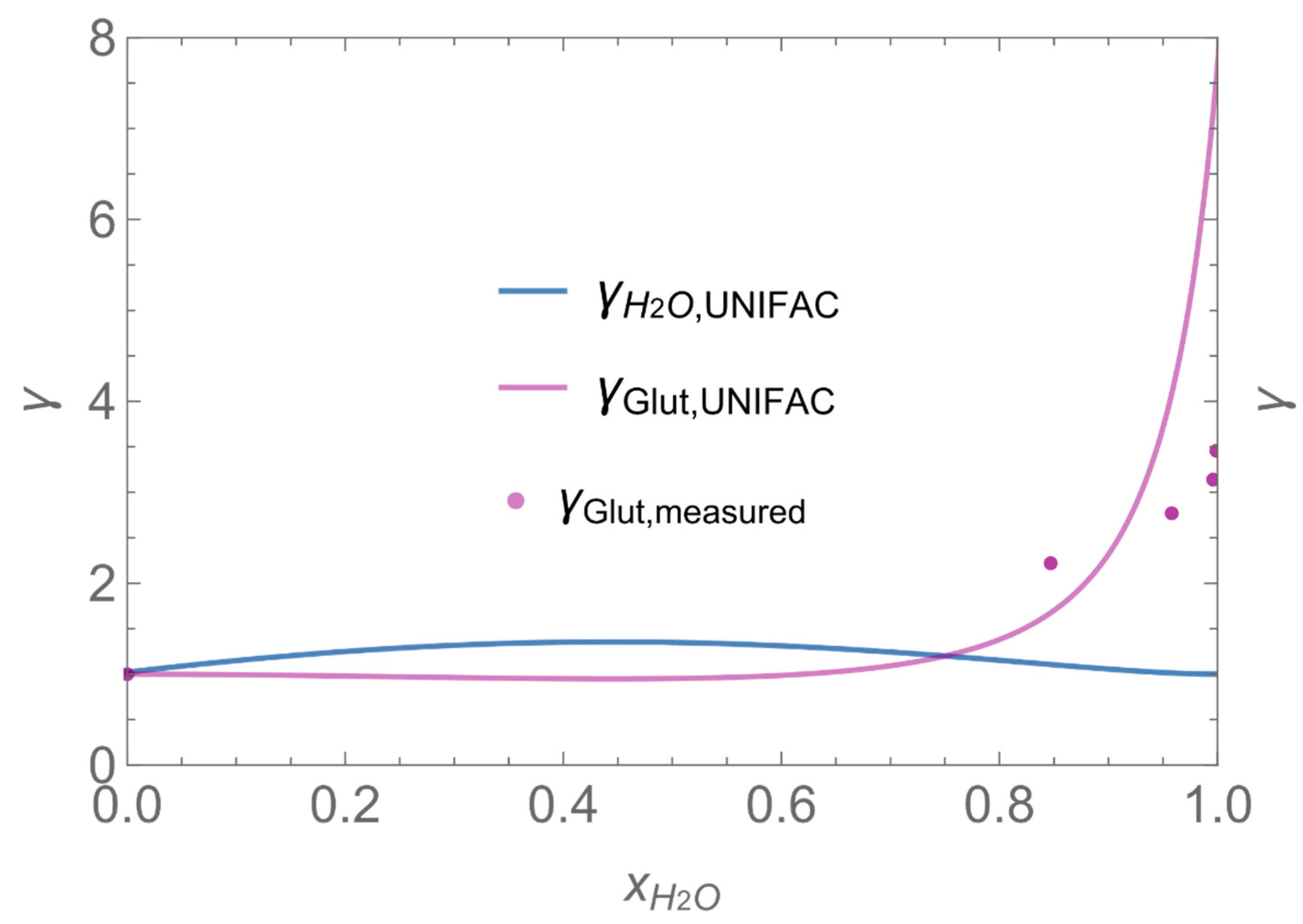
| γ | activity coefficient |
| surface area of the applied product [m2] | |
| mass transfer coefficient [m/s] | |
| ideal gas constant (8.3145 Pa m3 K−1 mol−1) | |
| temperature [K] | |
| volume of an air space [m3] | |
| velocity [m/s] | |
| molecular diffusion coefficient in air [m2/s] | |
| kinematic viscosity [m2/s] | |
| : | molecular weight [kg/mol] |
| n: | molar amount [mol] |
| w: | weight fraction |
| SC: | the initial surface coverage with the product or a compound [kg/m2] |
| C: | concentration [kg/m3] |
| t: | time [s] |
| Q: | air exchange rate [m3/s] |
| ACPH: | number of air changes [1/h] |
| r: | work rate (rate at which the surface is covered with product) [m2/s] |
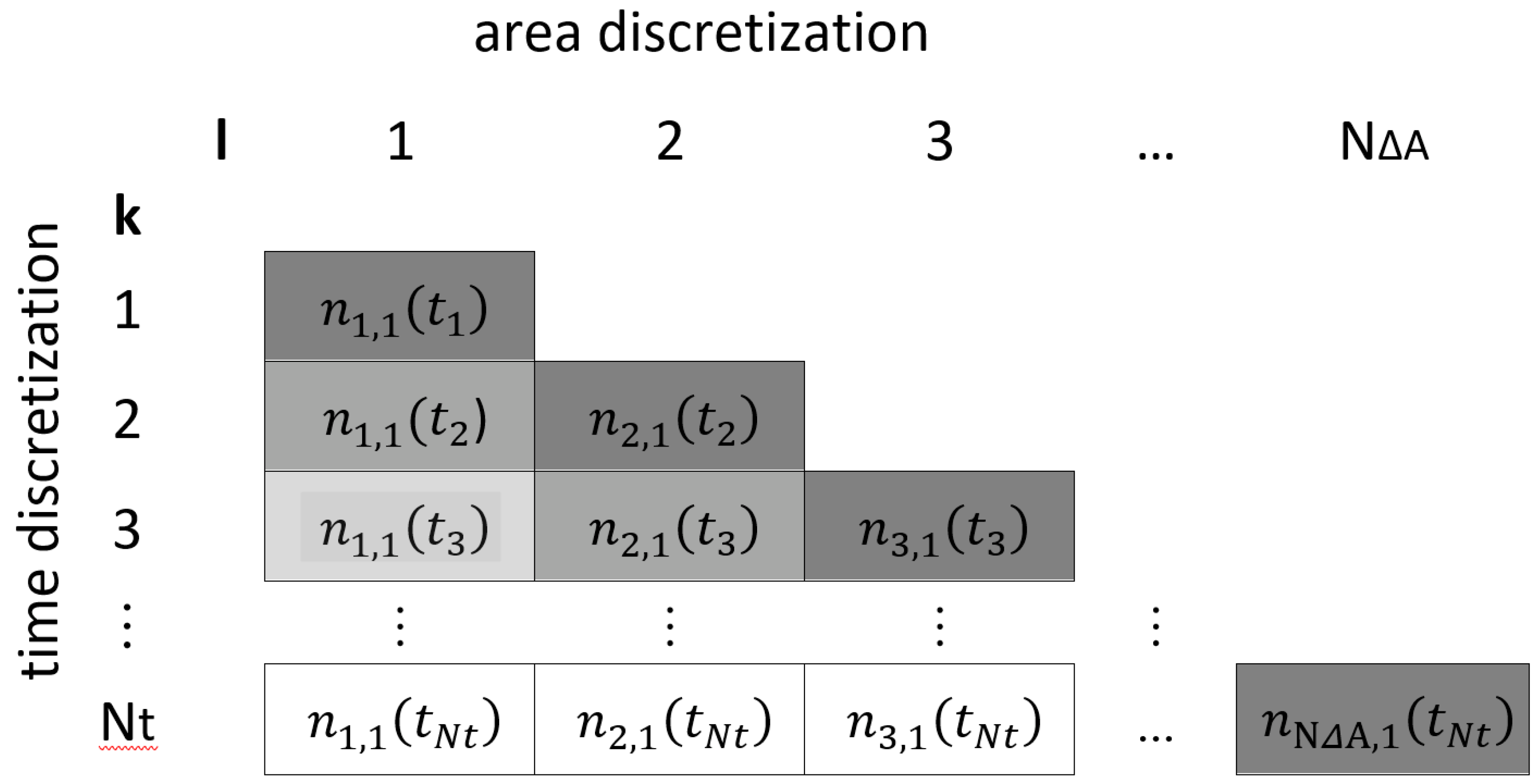
| Nt: | number of time steps |
| NΔA: | number of area elements |
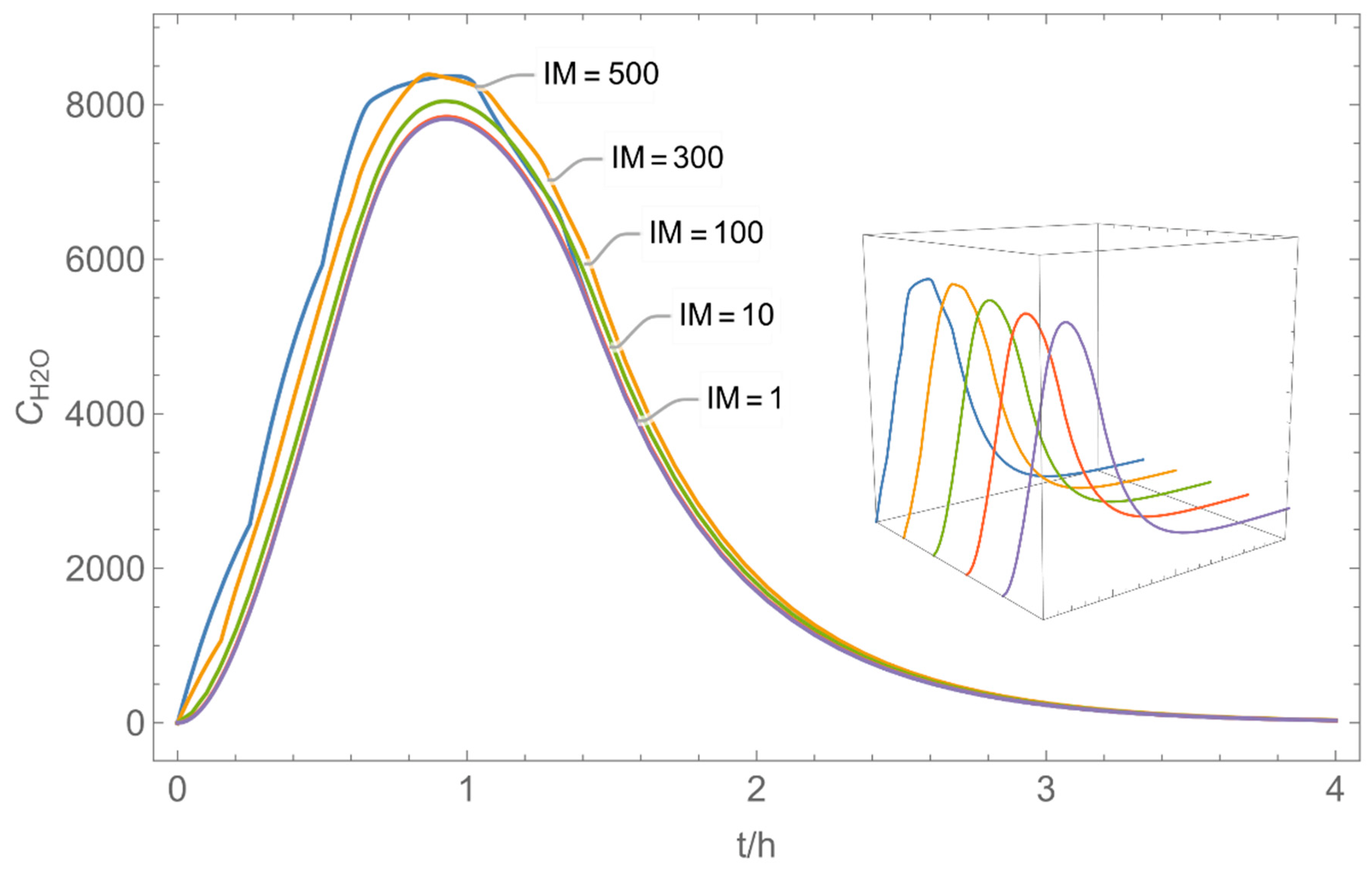
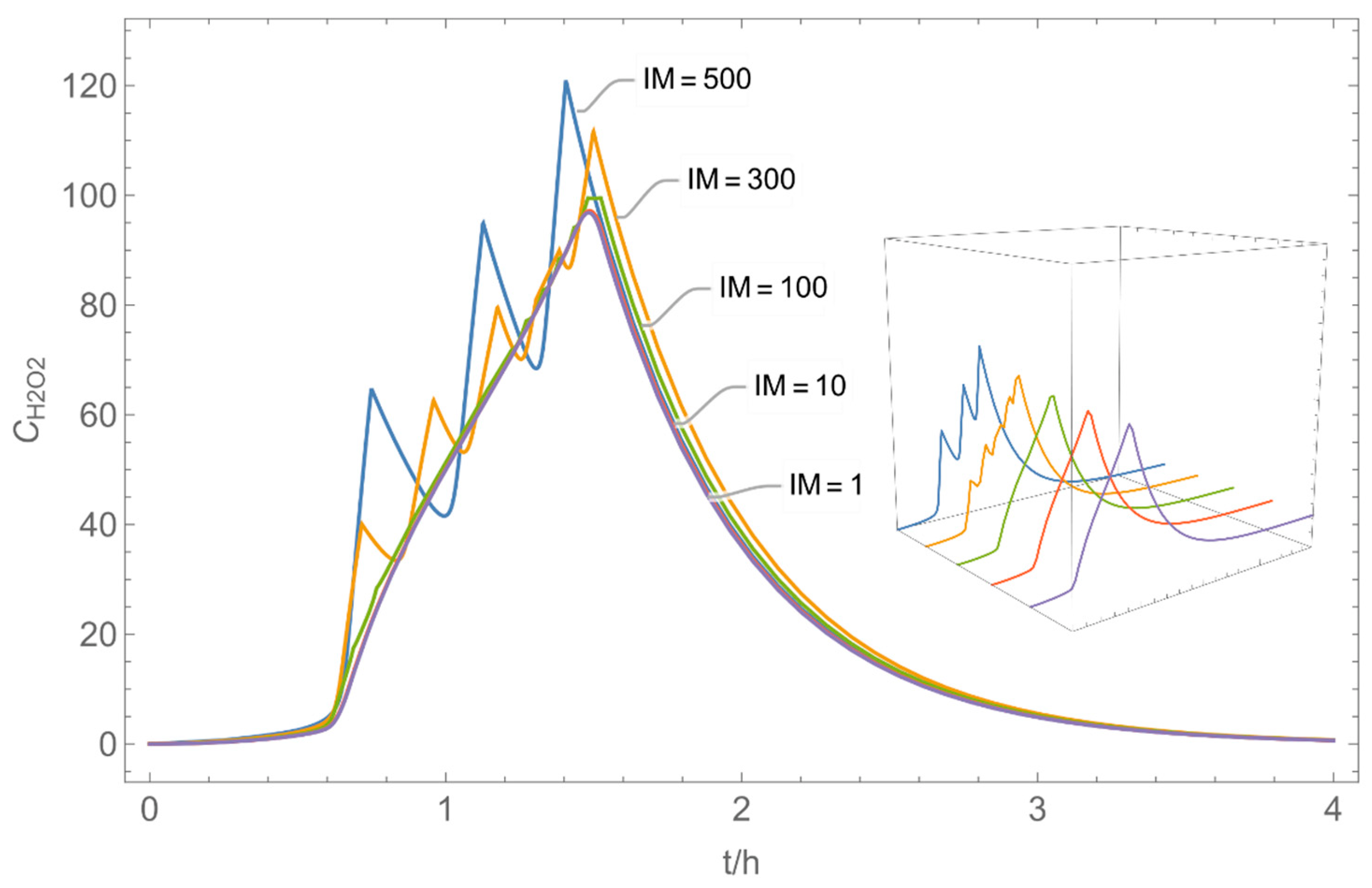
| IM: | integer multiples of Δt |
| NAC: | number of application cycles |
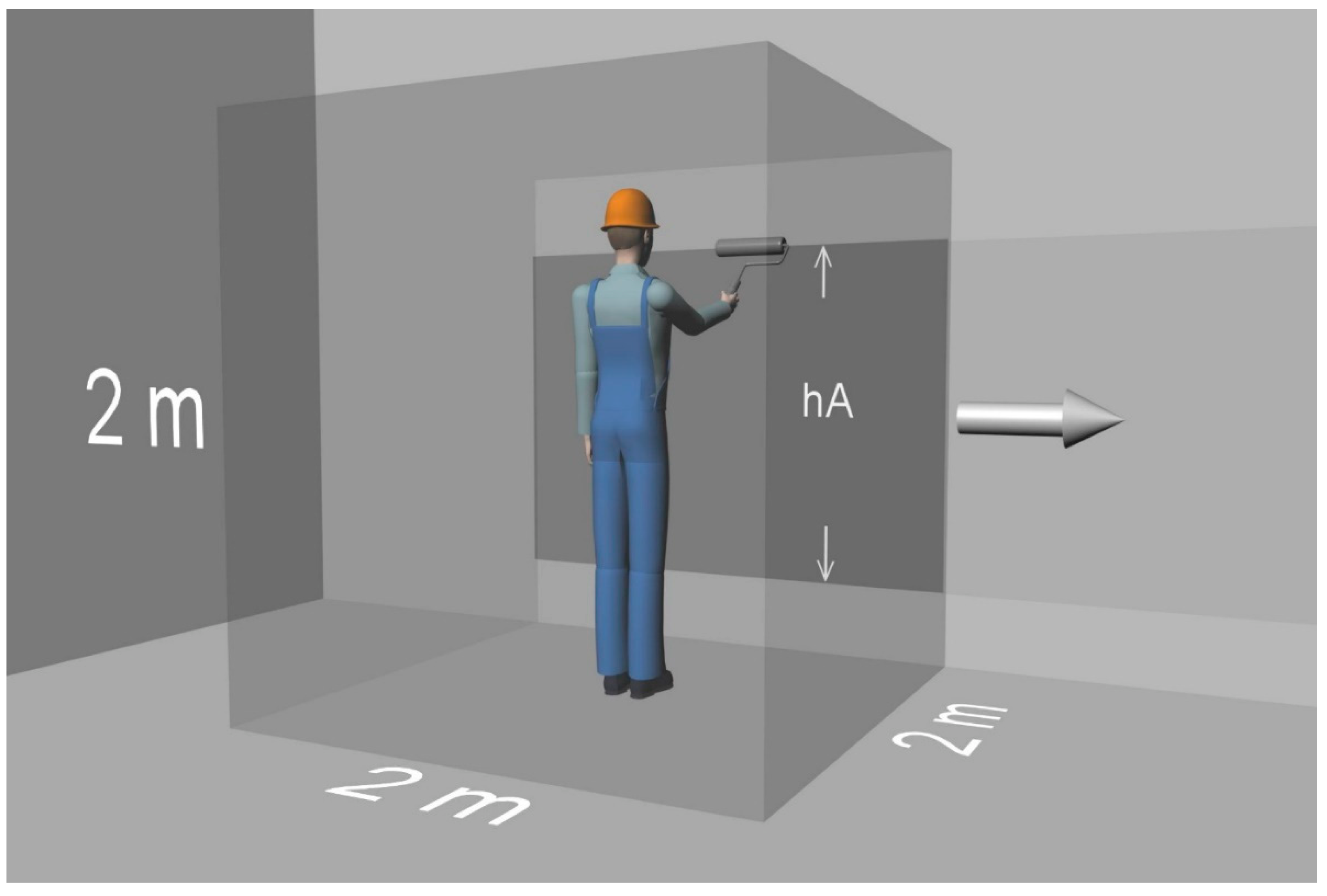
| hA: | height of the area to which the product is applied |
| T = 298.15 K | νair = 1.53∙10−5 m2/s | Vroom = 200 m3 |
| p*H2O = 3130 Pa | βH2O = 2.4∙10−3 m/s | Vnf = 8 m3 |
| p*H2O2 = 257 Pa | βH2O2 = 2.2∙10−3 m/s | Qnf/ff = 600 m3/h |
| p*glutarald. = 62 Pa | βglutarald. = 1.9∙10−3 m/s | ACPH = 2 /h |
| DH2O = 2.4∙10−5 m2/s | MH2O = 18∙10−3 kg/mol | r = 1 m2/min |
| DH2O2 = 1.8∙10−5 m2/s | MH2O2 = 34∙10−3 kg/mol | νair = 0.5 m/s |
| Dglutarald. = 0.73∙10−5 m2/s | Mglutarald. = 100∙10−3 kg/mol | SCP = 0.1 kg/m2 |
| η = 1.82∙10−5 kg/(m∙s) | wi = 0.01 | = 0 mg/m3 |
| № | Model/ Algorithm | Area A [m2] | Application Time/Pattern | Back-Pressure | Activity Coeff. |
|---|---|---|---|---|---|
| 1 | WMR_inst/ Runge-Kutta | 4 | instantaneous | with and without | with |
| 2 | WMR_inst/ Runge-Kutta | 40 | instantaneous | with and without | with |
| 3 | WMR_inst Runge-Kutta | 40 | instantaneous | with | with and without |
| 4 | WMR_kont/ Euler | 40 | continuous over 0.67 h (40 min) | with | with and without |
| 5 | NF/FF_inst/ Runge-Kutta | 4 | instantaneous | with | with |
| 6 | NF/FF_mov/ Euler | 40 | continuous over 0.67 h (40 min) | with | with |
| 7 | NF/FF_mov_int/ Euler | 40 | intermittent: ta,1 = 0 h, tb,1 = 0.25 h, ta,2 = 0.42 h, tb,2 = 0.67 h | with | with |
| № | H2O/H2O2 | H2O/Glutaraldehyde |
|---|---|---|
| 1 |  |  |
| 2 |  | 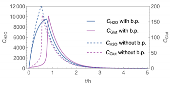 |
| 3 | 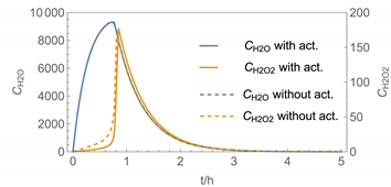 | 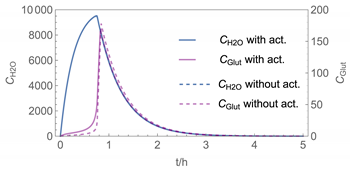 |
| 4 | 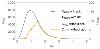 | 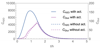 |
| 5 |  | 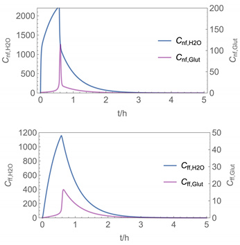 |
| 6 | 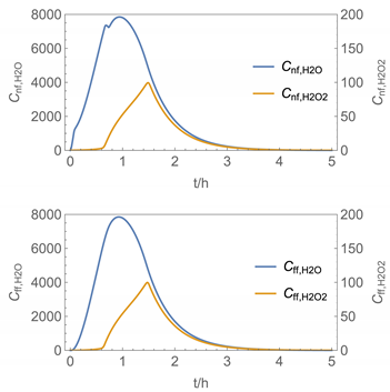 | 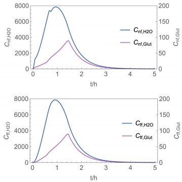 |
| 7 | 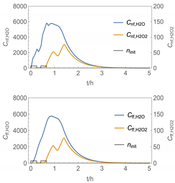 | 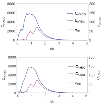 |
Publisher’s Note: MDPI stays neutral with regard to jurisdictional claims in published maps and institutional affiliations. |
© 2022 by the authors. Licensee MDPI, Basel, Switzerland. This article is an open access article distributed under the terms and conditions of the Creative Commons Attribution (CC BY) license (https://creativecommons.org/licenses/by/4.0/).
Share and Cite
Tischer, M.; Roitzsch, M. Estimating Inhalation Exposure Resulting from Evaporation of Volatile Multicomponent Mixtures Using Different Modelling Approaches. Int. J. Environ. Res. Public Health 2022, 19, 1957. https://doi.org/10.3390/ijerph19041957
Tischer M, Roitzsch M. Estimating Inhalation Exposure Resulting from Evaporation of Volatile Multicomponent Mixtures Using Different Modelling Approaches. International Journal of Environmental Research and Public Health. 2022; 19(4):1957. https://doi.org/10.3390/ijerph19041957
Chicago/Turabian StyleTischer, Martin, and Michael Roitzsch. 2022. "Estimating Inhalation Exposure Resulting from Evaporation of Volatile Multicomponent Mixtures Using Different Modelling Approaches" International Journal of Environmental Research and Public Health 19, no. 4: 1957. https://doi.org/10.3390/ijerph19041957
APA StyleTischer, M., & Roitzsch, M. (2022). Estimating Inhalation Exposure Resulting from Evaporation of Volatile Multicomponent Mixtures Using Different Modelling Approaches. International Journal of Environmental Research and Public Health, 19(4), 1957. https://doi.org/10.3390/ijerph19041957