
Spatial Clustering of County-Level COVID-19 Rates in the U.S.

 , , , ,
Abstract
:1. Introduction
2. Materials and Methods
2.1. Data and Measures
2.2. Geographic Information System (G.I.S.) Process
2.3. Statistical Analysis
3. Results
3.1. Overall Distribution of COVID-19 Cases
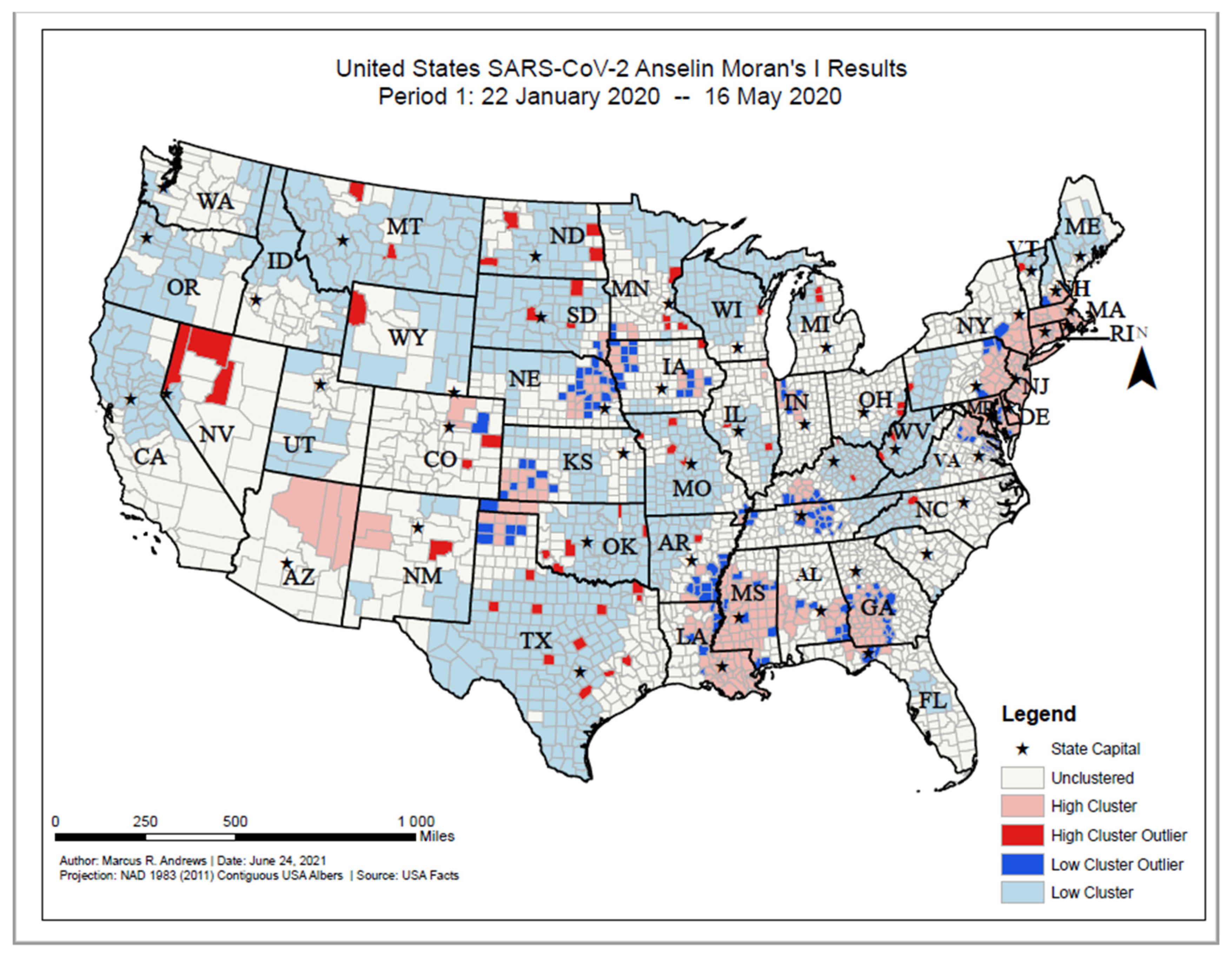
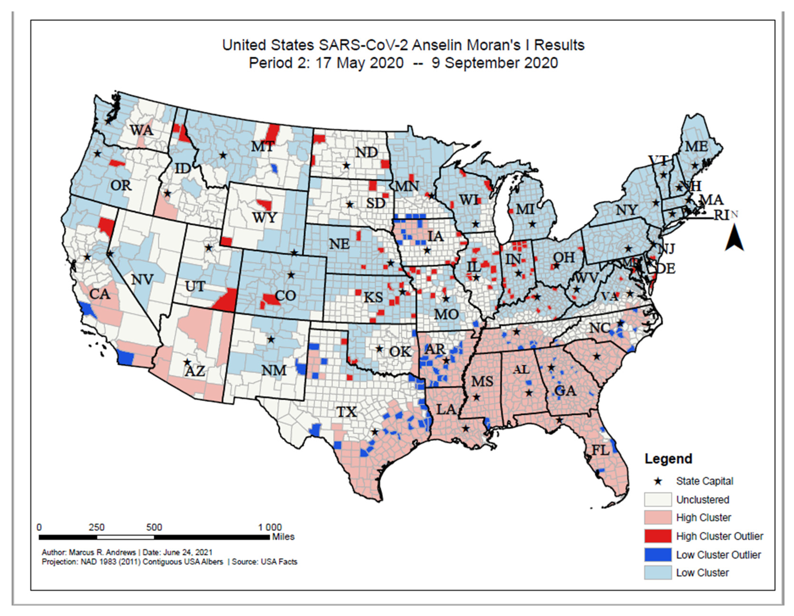
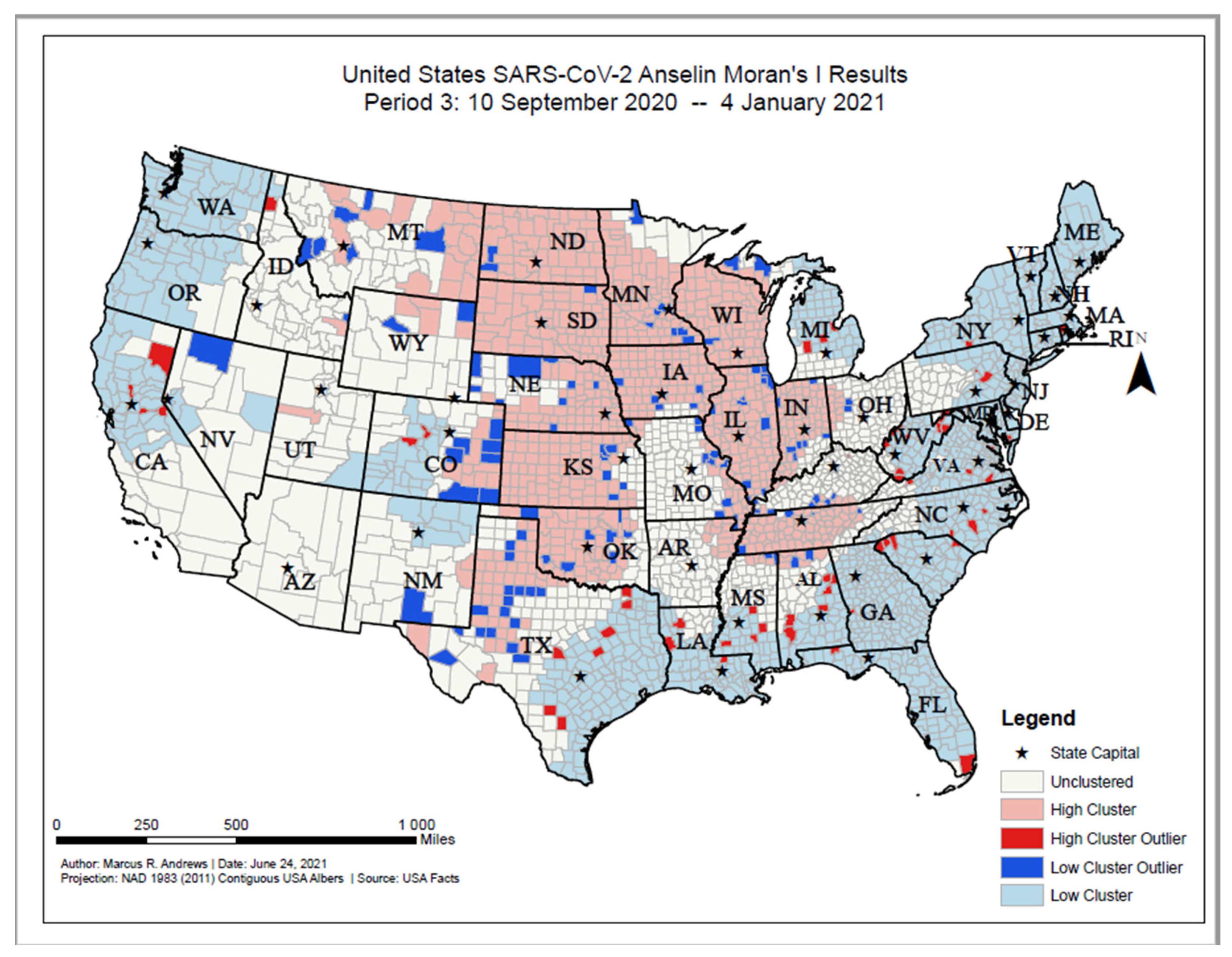
3.2. Anselin’s Local Moran’s I
3.3. Comparison of Clustering Characteristics
4. Discussion
5. Conclusions
Author Contributions
Funding
Institutional Review Board Statement
Informed Consent Statement
Data Availability Statement
Conflicts of Interest
Appendix A

| Source | Variable | Definition |
|---|---|---|
| Behavioral Risk Factor Surveillance System | Poor or Fair Health | Percentage of adults reporting fair or poor health (age-adjusted). |
| Adult smoking | Percentage of adults who are current smokers. | |
| United States Diabetes Surveillance System | Adult obesity | Percentage of the adult population (age 20 and older) that reports a body mass index (BMI) greater than or equal to 30 kg/m2. |
| Physical inactivity | Percentage of adults age 20 and over reporting no leisure-time physical activity. | |
| Diabetes prevalence | Percentage of adults aged 20 and above with diagnosed diabetes. | |
| US Department of Agriculture Food Environment Atlas, Map the Meal Gap from Feeding America | Food environment index | Index of factors that contribute to a healthy food environment, from 0 (worst) to 10 (best). |
| State-specific sources and EDFacts (U.S. Department of Education) | High school graduation | Percentage of ninth-grade cohort that graduates in four years. |
| Bureau of Labor Statistics | Unemployment | Percentage of population ages 16 and older unemployed but seeking work. |
| American Community Survey, 5-year estimates | Residential segregation—Black/White | Index of dissimilarity where higher values indicate greater residential segregation between Black and White county residents. |
| Homeownership | Percentage of occupied housing units that are owned. | |
| Severe housing cost burden | Percentage of households that spend 50% or more of their household income on housing. | |
| Some college | Percentage of adults ages 25–44 with some post-secondary education. | |
| Children in single-parent households | Percentage of children that live in a household headed by single parent. | |
| Comprehensive Housing Affordability Strategy (CHAS) data | Severe housing problems | Percentage of households with at least one of four housing problems: overcrowding, high housing costs, lack of kitchen facilities, or lack of plumbing facilities. |
| Map the Meal Gap | Food insecurity | Percentage of population who lack adequate access to food. |
| National Center for Health Statistics—Mortality Files | Life expectancy | Average number of years a person can expect to live. |
| Small Area Health Insurance Estimates | Uninsured adults | Percentage of population under age 65 without health insurance. |
| Median household income | The income where half of households in a county earn more and half of households earn less. | |
| Census Population Estimates | Race/Ethnicity Data | Percentage of population that falls within each racial/ethnic category |
| % Females | Percentage of population that is female. | |
| % Rural | Percentage of population living in a rural area. |
References
- Li, Q.; Guan, X.; Wu, P.; Wang, X.; Zhou, L.; Tong, Y.; Ren, R.; Leung, K.S.M.; Lau, E.H.Y.; Wong, J.Y.; et al. Early transmission dynamics in Wuhan, China, of novel coronavirus-infected pneumonia. N. Engl. J. Med. 2020. [Google Scholar] [CrossRef]
- Holshue, M.L.; DeBolt, C.; Lindquist, S.; Lofy, K.H.; Wiesman, J.; Bruce, H.; Spitters, C.; Keith Ericson, P.A.-C.; Sara Wilkerson, M.N.; Tural, A.; et al. First case of 2019 novel coronavirus in the United States. N. Engl. J. Med. 2020. [Google Scholar] [CrossRef] [PubMed]
- Lai, C.C.; Shih, T.P.; Ko, W.C.; Tang, H.J.; Hsueh, P.R. Severe acute respiratory syndrome coronavirus 2 (SARS-CoV-2) and coronavirus disease-2019 (COVID-19): The epidemic and the challenges. Int. J. Antimicrob. Agents 2020, 55, 105924. [Google Scholar] [CrossRef] [PubMed]
- Chang, D.; Lin, M.; Wei, L.; Xie, L.; Zhu, G.; Cruz, C.S.D.; Sharma, L. Epidemiologic and Clinical Characteristics of Novel Coronavirus Infections Involving 13 Patients Outside Wuhan, China. JAMA-J. Am. Med. Assoc. 2020, 323, 1092–1093. [Google Scholar] [CrossRef]
- World Health Organization. Rolling Updates on Coronavirus Disease (SARS-CoV-2). 2020. Available online: https://www.who.int/emergencies/diseases/novel-coronavirus-2019/events-as-they-happen (accessed on 26 June 2020).
- Wang, D.; Hu, B.; Hu, C.; Zhu, F.; Liu, X.; Zhang, J.; Wang, B.; Xiang, H.; Cheng, Z.; Xiong, Y.; et al. Clinical Characteristics of 138 Hospitalized Patients with 2019 Novel Coronavirus-Infected Pneumonia in Wuhan, China. JAMA-J. Am. Med. Assoc. 2020, 323, 1061–1069. [Google Scholar] [CrossRef] [PubMed]
- Chin, T.; Kahn, R.; Li, R.; Chen, J.; Krieger, N.; Buckee, C.O.; Balsari, S.; Kiang, M.U.S. county-level characteristics to inform equitable COVID-19 response. medRxiv 2020, 4. [Google Scholar] [CrossRef] [Green Version]
- WHO. Coronavirus Disease (COVID-19): Situation Report; World Health Organization: Genève, Switzerland, 2020. [Google Scholar]
- Ranney, M.L.; Griffeth, V.; Jha, A.K. Critical supply shortages-The need for ventilators and personal protective equipment during the COVID-19 pandemic. N. Engl. J. Med. 2020, 382, e41. [Google Scholar] [CrossRef]
- McMinn, S.; Carlsen, A.; Jaspers, B.; Talbot, R.; Adeline, S. In Large Texas Cities, Access to Coronavirus Testing May Depend on Where You Live. Houston Public Media. 2020. Available online: https://www.houstonpublicmedia.org/articles/news/2020/05/27/370633/in-large-texas-cities-access-to-coronavirus-testing-may-depend-on-where-you-live/ (accessed on 1 September 2021).
- Austin, J.C. COVID-19 Is Turning the Midwest’s Long Legacy of Segregation Deadly; Brookings Institute: Washington, DC, USA, 2020. [Google Scholar]
- Azar, K.; Shen, Z.; Romanelli, R.J.; Lockhart, S.H.; Smits, K.; Robinson, S.; Brown, S.; Pressman, A.R. Disparities In Outcomes Among COVID-19 Patients In A Large Health Care System In California. Health Aff. 2020, 39, 1253–1262. [Google Scholar] [CrossRef]
- Franch-Pardo, I.; Napoletano, B.M.; Rosete-Verges, F.; Billa, L. Spatial analysis and GIS in the study of COVID-19. A review. Sci. Total Environ. 2020, 739, 140033. [Google Scholar] [CrossRef]
- Schmidt, H. The Way We Ration Ventilators Is Biased Not every patient has a fair chance. The New York Times. 2020. Available online: https://indianactsi.org/review-the-way-we-ration-ventilators-is-biased-not-every-patient-has-a-fair-chance/ (accessed on 1 September 2021).
- Moghadas, S.M.; Shoukat, A.; Fitzpatrick, M.C.; Wells, C.R.; Sah, P.; Pandey, A.; Sachs, J.D.; Wang, Z.; Meyers, L.A.; Singer, B.H.; et al. Projecting hospital utilization during the COVID-19 outbreaks in the United States. Proc. Natl. Acad. Sci. USA 2020, 117, 9122–9126. [Google Scholar] [CrossRef] [PubMed] [Green Version]
- Gao, S.; Rao, J.; Kang, Y.; Liang, Y.; Kruse, J. Mapping county-level mobility pattern changes in the United States in response to COVID-19. SIGSpatial Spec. 2020, 12, 16–26. [Google Scholar] [CrossRef]
- Kamel Boulos, M.N.; Geraghty, E.M. Geographical tracking and mapping of coronavirus disease COVID-19/severe acute respiratory syndrome coronavirus 2 (SARS-CoV-2) epidemic and associated events around the world: How 21st century GIS technologies are supporting the global fight against outbr. Int. J. Health Geogr. 2020, 1–12. [Google Scholar] [CrossRef] [Green Version]
- Centers for Disease Control and Prevention. Health Equity Considerations and Racial and Ethnic Minority Groups. Centers for Disease Control and Prevention, 19 April 2021. Available online: https://www.cdc.gov/coronavirus/2019-ncov/community/health-equity/race-ethnicity.html (accessed on 1 September 2021).
- Gassman-Pines, A. American Inequality Meets COVID-19. The Economist. Available online: https://www.economist.com/united-states/2020/04/18/american-inequality-meets-covid-19 (accessed on 1 September 2021).
- Bilal, B.M.; Shahzad, A.; Komal, B.; Bashir, M.; Tan, D. Nexus between temperature and COVID-19 pandemic: A meta-analysis. In Proceedings of the 3rd International Electronic Conference on Environmental Research and Public Health—Public Health Issues in the Context of the COVID-19 Pandemic, online, 11–25 January 2021; MDPI: Basel, Switzerland. [Google Scholar] [CrossRef]
- Stringhini, S.; Carmeli, C.; Jokela, M.; Avendaño, M.; Muennig, P.; Guida, F.; Ricceri, F.; d’Errico, A.; Barros, H.; Bochud, M.; et al. LIFEPATH consortium. Socioeconomic status and the 25 × 25 risk factors as determinants of premature mortality: A multicohort study and meta-analysis of 1·7 million men and women. Lancet 2017, 389, 1229–1237. [Google Scholar] [CrossRef] [Green Version]
- Benfer, E.A.; Wiley, L.F. Health Justice Strategies To Combat COVID-19: Protecting Vulnerable Communities During A Pandemic. Health Aff. 2020, 10. [Google Scholar] [CrossRef]
- Richardson, S.; Hirsch, J.S.; Narasimhan, M.; Crawford, J.M.; McGinn, T.; Davidson, K.W.; the Northwell COVID-19 Research Consortium; Barnaby, D.P.; Becker, L.B.; Chelico, J.D.; et al. Presenting Characteristics, Comorbidities, and Outcomes among 5700 Patients Hospitalized with COVID-19 in the New York City Area. JAMA-J. Am. Med. Assoc. 2020, 323, 2052–2059. [Google Scholar] [CrossRef] [PubMed]
- Henry-Nickle, M.; Hudak, J. Social Distancing in Black and White Neighborhoods in Detroit: A Data-Driven Look at Vulnerable Communities; Brookings Institute: Washington, DC, USA, 2020. [Google Scholar]
- Karmakar, M.; Lantz, P.M.; Tipirneni, R. Association of Social and Demographic Factors with COVID-19 Incidence and Death Rates in the US. JAMA Netw. Open 2021, 4, e2036462. [Google Scholar] [CrossRef]
- Dyer, O. COVID-19: Black people and other minorities are hardest hit in US. BMJ 2020, 369. [Google Scholar] [CrossRef] [Green Version]
- Webb Hooper, M.; Nápoles, A.M.; Pérez-Stable, E.J. COVID-19 and Racial/Ethnic Disparities. JAMA-J. Am. Med. Assoc. 2020, 323, 2466–2467. [Google Scholar] [CrossRef] [PubMed]
- Gross, C.P.; Essien, U.R.; Pasha, S.; Gross, J.R.; Wang, S.Y.; Nunez-Smith, M. Racial and Ethnic Disparities in Population-Level COVID-19 Mortality. J. Gen. Intern. Med. 2020, 35, 3097–3099. [Google Scholar] [CrossRef]
- Garg, S.; Kim, L.; Whitaker, M.; O’Halloran, A.; Cummings, C.; Holstein, R.; Prill, M.; Chai, S.J.; Kirley, P.D.; Alden, N.B.; et al. Hospitalization Rates and Characteristics of Patients Hospitalized with Laboratory-Confirmed Coronavirus Disease 2019—COVID-NET. MMWR Morb. Mortal. Wkly. Rep. 2020, 69, 458. [Google Scholar] [CrossRef] [PubMed]
- Wadhera, R.K.; Wadhera, P.; Gaba, P.; Figueroa, J.F.; Maddox KE, J.; Yeh, R.W.; Shen, C. Variation in COVID-19 Hospitalizations and Deaths Across New York City Boroughs. JAMA-J. Am. Med. Assoc. 2020, 323, 2192–2195. [Google Scholar] [CrossRef]
- Williams, D.R.; Rucker, T.D. Understanding and addressing racial disparities in health care. Health Care Financ. Rev. 2000, 21, 75–90. [Google Scholar] [PubMed]
- Mollalo, A.; Vahedi, B.; Rivera, K.M. GIS-based spatial modeling of COVID-19 incidence rate in the continental United States. Sci. Total Environ. 2020, 728, 138884. [Google Scholar] [CrossRef] [PubMed]
- Brunsdont, C.; Fotheringham, S.; Charlton, M. Geographically weighted regression-Modelling spatial non-stationarity. J. R. Stat. Soc. Ser. D Stat. 1998, 47, 431–443. [Google Scholar] [CrossRef]
- Ma, K.C.; Menkir, T.F.; Kissler, S.; Grad, Y.H.; Lipsitch, M. Modeling the impact of racial and ethnic disparities on COVID-19 epidemic dynamics. Elife 2021, 10, e66601. [Google Scholar] [CrossRef]
- Torrats-Espinosa, G. Using machine learning to estimate the effect of racial segregation on COVID-19 mortality in the United States. Proc. Natl. Acad. Sci. USA 2021, 118, e2015577118. [Google Scholar] [CrossRef] [PubMed]
- United States Census Bureau. American Community Survey. 2010. Available online: https://factfinder.census.gov/faces/nav/jsf/pages/searchresults.xhtml?refresh=t (accessed on 20 November 2020).
- Fleiss, J.L. Statistical Methods for Rates and Proportions, 2nd ed.; Wiley: New York, NY, USA, 1981. [Google Scholar]
- Robert Wood Johnson Foundation. County Health Rankings. 2020. Available online: https://www.countyhealthrankings.org (accessed on 20 November 2020).
- Pan, W.; Miyazaki, Y.; Tsumura, H.; Miyazaki, E.; Yang, W. Identification of county-level health factors associated with COVID-19 mortality in the United States. J. Biomed. Res. 2020, 34, 437. [Google Scholar] [CrossRef]
- Andrews, M.R.; Tamura, K.; Claudel, S.E.; Xu, S.; Ceasar, J.N.; Collins, B.S.; Langerman, S.; Mitchell, V.M.; Baumer, Y.; Powell-Wiley, T.M. Geospatial analysis of neighborhood deprivation index (NDI) for the United States by county. J. Maps 2020, 16, 101–112. [Google Scholar] [CrossRef]
- Congdon, P. Variations in obesity rates between US counties: Impacts of activity access, food environments, and settlement patterns. Int. J. Environ. Res. Public Health 2017, 14, 1023. [Google Scholar] [CrossRef] [Green Version]
- Li, D.; Gaynor, S.M.; Quick, C.; Chen, J.T.; Stephenson, B.J.; Coull, B.A.; Lin, X. Identifying US County-level characteristics associated with high COVID-19 burden. BMC Public Health 2021, 21, 1–10. [Google Scholar] [CrossRef]
- Andrews, M.R.; Ceasar, J.; Tamura, K.; Langerman, S.D.; Mitchell, V.M.; Collins, B.S.; Baumer, Y.; Huerta, C.A.G.; Dey, A.K.; Playford, M.P.; et al. Neighborhood environment perceptions associate with depression levels and cardiovascular risk among middle-aged and older adults: Data from the Washington, DC cardiovascular health and needs assessment. Aging Ment. Health 2020, 25, 2078–2089. [Google Scholar] [CrossRef] [PubMed]
- Allen, D. GIS Tutorial 2: Spatial Analysis Workbook, 4th ed.; Esri Press: Redlands, CA, USA, 2016. [Google Scholar]
- Esri. What Is a z-Score? What Is a p-Value?-ArcGIS Pro|Documentation, Esri. Available online: https://pro.arcgis.com/en/pro-app/latest/tool-reference/spatial-statistics/what-is-a-z-score-what-is-a-p-value.htm (accessed on 20 November 2020).
- Anselin, L. Local Indicators of Spatial Association—LISA. Geogr. Anal. 1995, 27, 93–115. [Google Scholar] [CrossRef]
- Tamura, K.; Puett, R.C.; Hart, J.E.; Starnes, H.A.; Laden, F.; Troped, P.J. Spatial clustering of physical activity and obesity in relation to built environment factors among older women in three U.S. states. BMC Public Health 2014, 14, 1–16. [Google Scholar] [CrossRef] [PubMed] [Green Version]
- Simons, R.L.; Lei, M.; Beach, S.R.H.; Barr, A.B.; Simons, L.G.; Gibbons, F.X.; Philibert, R.A. Discrimination, segregation, and chronic inflammation: Testing the weathering explanation for the poor health of Black Americans. Dev. Psychol. 2018, 54, 1993–2006. [Google Scholar] [CrossRef]
- Paradies, Y. A systematic review of empirical research on self-reported racism and health. Int. J. Epidemiol. 2006, 35, 888–901. [Google Scholar] [CrossRef] [PubMed] [Green Version]
- Centers for Disease Control and Prevention. Health Equity Considerations & Racial & Ethnic Minority Groups; Centers for Disease Control and Prevention: Atlanta, GA, USA, 2020. [Google Scholar]
- Baumer, Y.; Farmer, N.; Premeaux, T.A.; Wallen, G.R.; Powell-Wiley, T.M. Health disparities in COVID-19: Addressing the role of social determinants of health in immune system dysfunction to turn the tide. Front. Public Health 2020, 8, 589. [Google Scholar] [CrossRef] [PubMed]
- Centers for Disease Control and Prevention. CDC Activities and Initiatives Supporting the COVID-19 Response and the President’s Plan for Opening America Up Again; Centers for Disease Control and Prevention: Atlanta, GA, USA, 2020. [Google Scholar]
- Saffary, T.; Adegboye, O.A.; Gayawan, E.; Elfaki, F.; Kuddus, M.A.; Saffary, R. Analysis of COVID-19 Cases’ Spatial Dependence in US Counties Reveals Health Inequalities. Front. Public Health 2020, 8, 579190. [Google Scholar] [CrossRef] [PubMed]
- Mahajan, U.V.; Larkins-Pettigrew, M. Racial demographics and COVID-19 confirmed cases and deaths: A correlational analysis of 2886 US counties. J. Public Health 2020, 42, 445–447. [Google Scholar] [CrossRef]
- Waller, L.A.; Gotway, C.A. Applied Spatial Statistics for Public Health Data; Wiley: New York, NY, USA, 2004; Volume 100. [Google Scholar] [CrossRef]
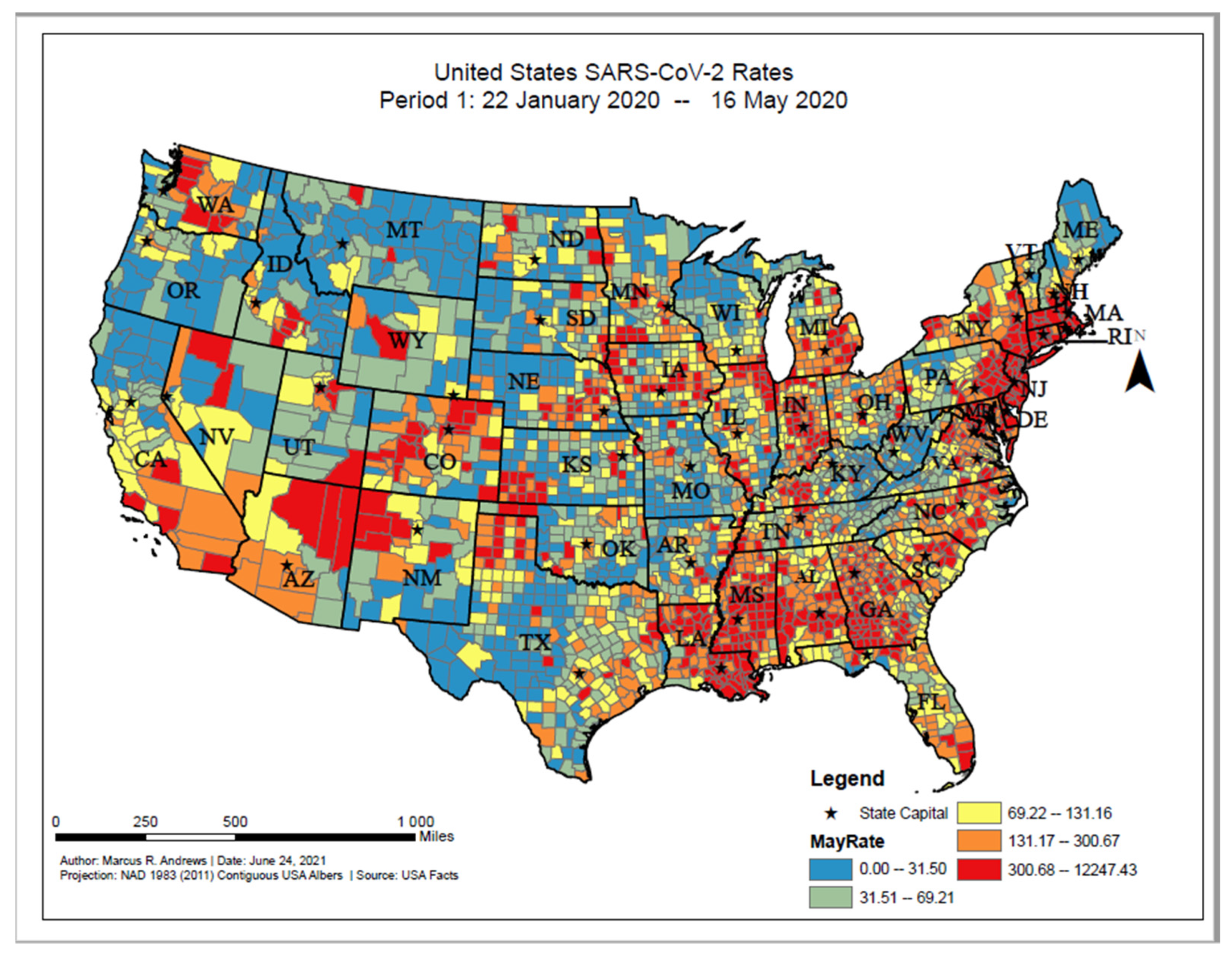


| Time Point 1: Rates from 22 January–16 May 2020 Results | |||||
|---|---|---|---|---|---|
| Unclustered (n = 1531) | High COVID-19 Rate Clusters (n = 349) | Low COVID-19 Rate Clusters (n = 1021) | High COVID-19 Rate Outlier (n = 57) | Low COVID-19 Rate Outlier (n = 150) | |
| Range | |||||
| Characteristics (S.D.) | |||||
| Cases per 100,000 people |
228.13 (534.16) |
855.73 (788.15) *** |
47.75 (45.53) *** |
452.50 (216.06) ** |
133.67 (63.33) * |
| % Rural |
56.49% (31.12%) |
45.96% (33.57%) *** |
64.72% (29.76%) *** |
54.39% (30.74%) |
68.20% (28.72%) *** |
| % Female |
49.94% (2.17%) |
50.64% (2.43%) *** |
49.72% (2.08%) * |
48.56% (4.02%) *** |
50.01% (2.33%) |
| % of Age Group (S.D.) | |||||
| % under 18 |
22.00% (3.26%) |
22.69% (3.25%) ** |
21.90% (3.76%) |
22.19% (3.16%) |
22.31% (2.86%) |
| % 65 and older |
19.05% (4.50%) |
17.21% (3.50%) *** |
20.52% (5.02%) *** |
18.47% (4.36%) |
19.15% (4.27%) |
| Race/Ethnicity (S.D.) | |||||
| % White |
76.66% (18.36%) |
61.02% (20.60%) *** |
81.00% (19.56%) *** |
75.19% (19.03%) |
77.33% (17.67%) |
| % Black |
9.94% (13.81%) |
23.34% (21.92%) *** |
2.43% (3.62%) *** |
4.74% (5.37%) * |
14.07% (17.25%) ** |
| % Native American |
1.27% (3.45%) |
1.64% (7.58%) |
3.40% (9.67%) *** |
3.42% (7.76%) *** |
0.50% (0.68%) * |
| % Asian |
1.53% (2.60%) |
2.62% (3.91%) *** |
1.06% (1.73%) *** |
1.32% (1.65%) |
1.01% (1.86%) |
| % Hispanic |
9.27% (12.47%) |
10.17% (11.57%) |
10.50% (16.91%) * |
14.00% (15.82%) * |
5.66% (5.83%) * |
| % Native Hawaiian/Pacific Islander |
0.02% (0.17%) |
0.01% (0.13%) |
0.04% (0.24%) * |
0.07% (0.26%) * |
0.01% (0.08%) |
| Black/White Segregation |
44.61 (16.55) |
42.53 (15.96) * |
49.97 (15.02) *** |
47.07 (15.67) |
35.11 (16.33) *** |
| Median Household Income |
53,674.39 (13,082.72) |
56,927.61 (21,725.10) * |
49,665.37 (10,315.00) *** |
52,178.53 (12,946.71) |
52,934.70 (14,757.76) |
| Community Characteristics (S.D.) | |||||
| High School Graduation Rate |
88.76% (6.51%) |
86.59% (7.33%) *** |
89.64% (7.58%) * |
89.02% (6.34%) |
89.80% (7.91%) |
| % Some College |
58.43% (11.60%) |
57.54% (13.10%) |
57.25% (11.33%) ** |
55.63% (13.40%) |
58.46% (13.50%) |
| % Homeowners |
71.52% (7.83%) |
68.92% (9.86%) *** |
72.54% (7.50%) ** |
70.21% (8.16%) |
71.61% (9.31%) |
| % Single Parent Household |
32.41% (9.92%) |
38.55% (14.45%) *** |
30.28% (9.22%) *** |
30.89% (7.38%) |
31.69% (12.10%) |
| % Severe Housing Issues |
13.69% (3.86%) |
15.94% (4.67%) *** |
13.27% (4.12%) * |
12.35% (3.83%) * |
12.65% (3.99%) ** |
| % Severe Housing Cost Burden |
11.28% (3.44%) |
13.45% (4.12%) *** |
10.64% (3.26%) *** |
10.12% (3.41%) * |
10.95% (3.95%) |
| % Food Insecure |
13.08% (3.57%) |
14.53% (6.33%) *** |
13.12% (3.15%) |
12.65% (3.63%) |
13.81% (5.11%) * |
| Food Environment Index |
7.56 (0.99) |
7.26 (1.61) *** |
7.39 (1.063) *** |
7.55 (1.12) |
7.43 (1.43) |
| % Uninsured |
12.93% (5.80%) |
13.60% (6.41%) |
14.34% (6.67%) *** |
15.16% (7.50%) ** |
13.05% (4.82%) |
| % Unemployed |
4.02% (1.30%) |
4.47% (1.60%) *** |
4.15% (1.49%) * |
3.84% (1.28%) |
3.83% (1.49%) |
| County Level Health Related factors (S.D.) | |||||
| Life Expectancy |
77.64 (2.91) |
77.30 (3.35) |
77.25 (3.03) ** |
77.87 (3.44) |
77.13 (2.86) * |
| % Adults with Diabetes |
12.14% (4.01%) |
12.68% (4.46%) * |
12.04% (3.94%) |
12.32% (4.63%) |
12.81% (4.22%) |
| % Fair or Poor Health |
17.48% (4.14%) |
19.63% (5.99%) *** |
18.00% (4.81%) ** |
17.75% (4.63%) |
18.48% (5.70%) ** |
| % Smokers |
17.22% (3.10%) |
17.81% (3.98%) ** |
17.56% (4.01%) * |
17.23% (3.30% |
18.13% (3.76%) ** |
| % Adults with Obesity |
32.90% (5.41%) |
33.47% (6.31%) |
32.43% (4.98%) * |
32.77% (6.77%) |
34.83% (5.34%) *** |
| % Physically Inactive |
27.30% (5.76%) |
28.16% (6.22%) * |
27.26% (5.18%) |
26.51% (6.27%) |
29.47% (6.36%) *** |
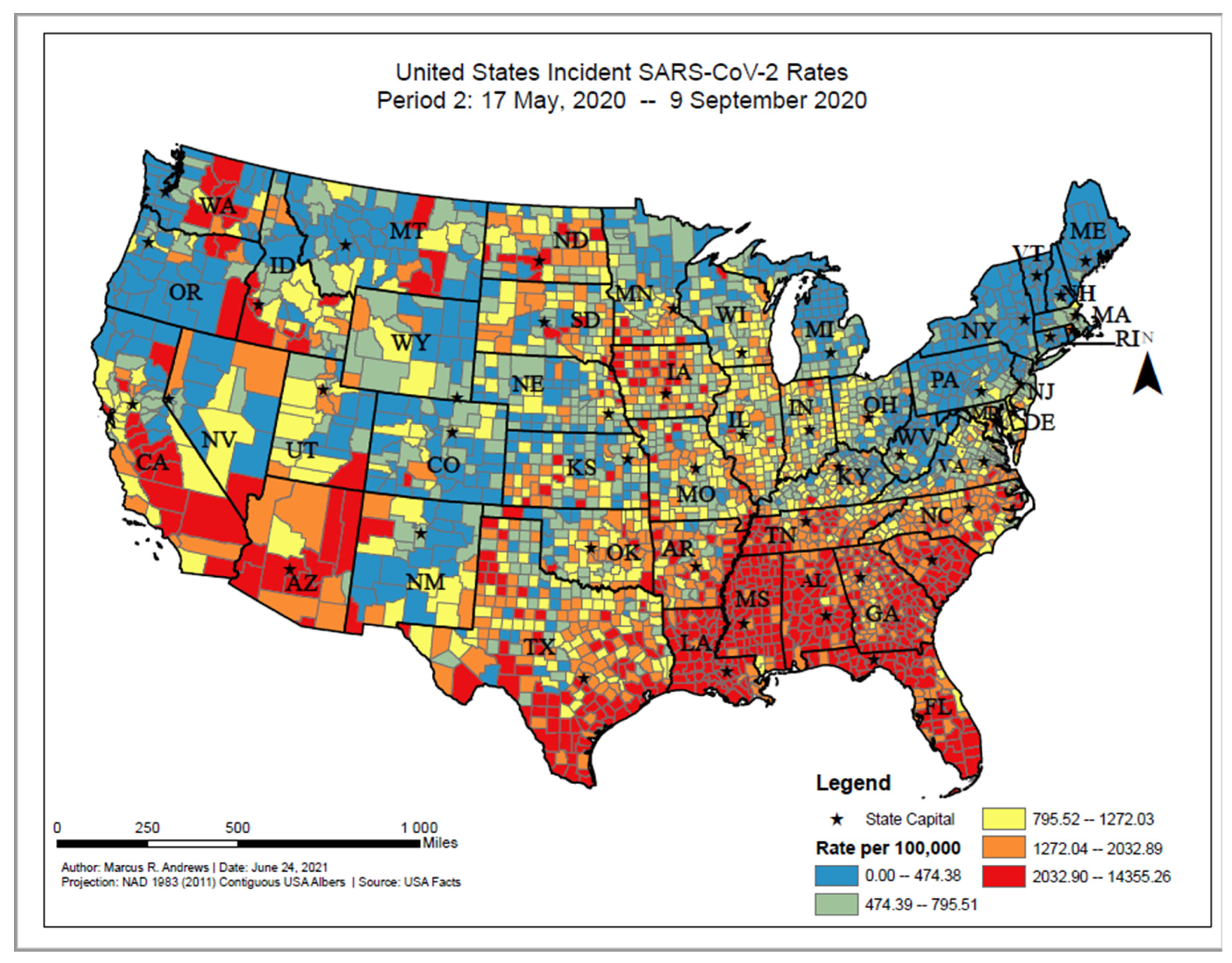
| Time Point 2: Rates from 17 May–9 September 2020 Results Incident Case Cluster | |||||
|---|---|---|---|---|---|
| Unclustered (n = 946) | High COVID-19 Rate Clusters (n = 717) | Low COVID-19 Rate Clusters (n = 1238) | High COVID-19 Rate Outlier (n = 109) | Low COVID-19 Rate Outlier (n = 114) | |
| Range | |||||
| Characteristics (SD) | |||||
| Cases per 100,000 people | 1264.75 (793.22) | 2715.26 (1311.74) *** | 565.76 (310.83) *** | 1757.13 (429.08) *** | 1039.71 (232.85) * |
| % Rural | 58.94% (33.65%) | 56.80% (28.95%) | 59.53% (30.87%) | 47.70% (33.61%) ** | 66.87% (27.97%) * |
| % Female | 49.73% (2.09%) | 50.23% (2.91%) *** | 49.84% (1.96%) | 50.16% (2.03%) * | 50.39% (1.43%) * |
| % of Age Group (S.D.) | |||||
| % under 18 | 22.90% (3.86%) | 22.53% (3.11%) * | 21.15% (3.03%) *** | 22.44% (3.40%) | 21.70% (2.87%) * |
| % 65 and older | 19.21% (5.00%) | 18.07% (4.40%) *** | 20.15% (4.36%) *** | 17.78% (4.21%) * | 20.70% (5.17%) * |
| Race/Ethnicity (S.D.) | |||||
| % White | 75.90% (19.50%) | 60.87% (20.52%) *** | 85.59% (13.49%) *** | 79.41% (16.03%) | 73.41% (18.16%) |
| % Black | 4.94% (8.88%) | 24.12% (19.60%) *** | 3.44% (5.60%) *** | 7.08% (10.81%) * | 12.42% (14.45%) *** |
| % Native American | 3.40% (9.56%) | 1.15% (4.14%) *** | 1.57% (5.36%) *** | 1.53% (5.11%) * | 1.21% (2.53%) * |
| % Asian | 1.65% (3.20%) | 1.20% (1.53%) ** | 1.46% (2.47%) | 1.81% (2.31%) | 1.30% (2.18%) |
| % Hispanic | 12.65% (15.43%) | 11.50% (17.81%) | 6.42% (8.91%) *** | 8.54% (8.26%) *** | 10.47% (13.51%) |
| % Native Hawaiian/Pacific Islander | 0.05% (0.25%) | 0.02% (0.19%) * | 0.02% (0.14%) ** | 0.04% (0.19%) | 0.01% (0.10%) |
| Black/White Segregation | 46.0475 (15.36) | 37.0831 (14.38) *** | 52.8096 (15.10) *** | 49.4997 (16.15) * | 34.6357 (15.19) *** |
| Median Household Income | 54,365.72 (13,835.57) | 46,256.74 (11,294.04) *** | 55,251.09 (14,359.52) | 52,879.94 (9623.77) | 50,052.32 (12,506.54) ** |
| Community Characteristics (S.D.) | |||||
| High School Graduation Rate | 89.60% (7.37%) | 86.94% (6.95%) *** | 89.29% (6.84%) | 89.46% (6.50%) | 89.88% (6.81%) |
| % Some College | 59.32% (11.78%) | 51.41% (11.15%) *** | 60.66% (10.71%) * | 59.80% (11.91%) | 54.47% (12.31%) *** |
| % Homeowners | 71.48% (8.08%) | 69.50% (8.34%) *** | 72.87% (7.60%) *** | 67.97% (9.84%) *** | 74.32% (6.73%) ** |
| % Single Parent Household | 29.56% (9.77%) | 40.28% (11.66%) *** | 29.87% (8.40%) *** | 31.87% (8.97%)* | 32.81% (9.67%) ** |
| % Severe Housing Issues | 13.25% (4.44%) | 15.21% (3.76%) | 13.27% (3.94%) | 13.74% (4.00%) | 13.38% (3.67%) |
| % Severe Housing Cost Burden | 10.53% (3.59%) | 12.49% (3.55%) *** | 11.17% (3.47%) *** | 11.21% (3.60%) | 10.96% (3.38%) |
| % Food Insecure | 12.49% (3.61%) | 16.17% (4.72%) *** | 12.11% (2.73%) * | 12.94% (2.95%) | 14.92% (4.42%) *** |
| Food Environment Index | 7.512 (1.17) | 6.910 (1.20) *** | 7.759 (0.92) *** | 7.600 (0.90) | 7.148 (1.24) ** |
| % Uninsured | 14.65% (6.66%) | 17.53% (5.41%) *** | 10.21% (4.25%) *** | 12.13% (4.91%) *** | 16.37% (6.49%) * |
| % Unemployed | 3.70% (1.30%) | 4.59% (1.54%) *** | 4.15% (1.35%) *** | 3.78% (1.34%) | 4.10% (1.24%) * |
| County Level Health Related factors (S.D.) | |||||
| Life Expectancy | 77.8875 (3.12) | 75.94 (2.56) *** | 78.05 (2.94) | 77.56 (2.52) | 76.97 (2.61) * |
| % Adults with Diabetes | 11.46% (3.93%) | 14.35% (4.22%) *** | 11.43% (3.49%) | 11.83% (3.59%) | 13.94% (5.25%) *** |
| % Fair or Poor Health | 17.04% (4.23%) | 21.90% (4.75%) *** | 16.32% (3.84%) *** | 17.39% (3.61%) | 19.07% (4.11%) *** |
| % Smokers | 16.48% (3.67%) | 19.18% (3.19%) *** | 17.15% (3.43%) *** | 17.94% (3.08%) *** | 17.22% (2.87%) * |
| % Adults with Obesity | 32.06% (5.00%) | 35.26% (5.59%) *** | 32.02% (5.27%) | 33.80% (4.67%) ** | 33.96% (5.75%) ** |
| % Physically Inactive | 26.55% (5.11%) | 30.85% (5.72%) *** | 26.08% (5.31%) * | 26.84% (4.96%) | 29.88% (5.75%) *** |
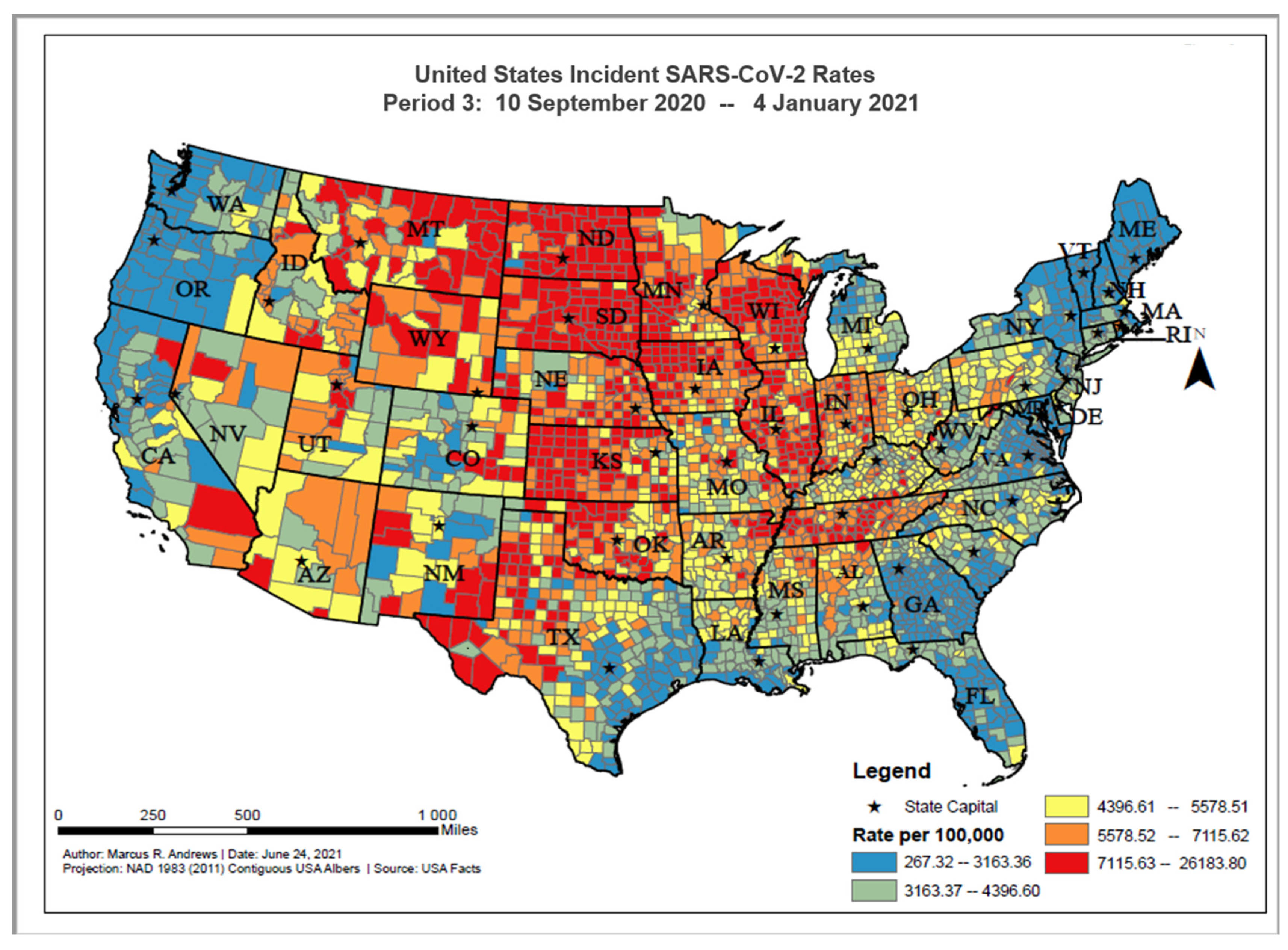
| Time Point 3: Rates from 10 September–4 January 2021 Results Incident Case Cluster | |||||
|---|---|---|---|---|---|
| Unclustered (n = 895) | High COVID-19 Rate clusters (n = 921) | Low COVID-19 Rate clusters (n = 1103) | High COVID-19 Rate Outlier (n = 65) | Low COVID-19 Rate Outlier (n = 124) | |
| Range | |||||
| Characteristics (S.D.) | |||||
| Cases per 100,000 people | 5327.78 (1605.30) |
7804.44 (2106.94) *** |
3088.61 (1058.54) *** |
6069.39 (1060.79) ** |
4472.66 (785.93) *** |
| % Rural |
59.33% (30.31%) |
64.02% (29.78%) ** |
52.27% (32.03%) *** |
57.49% (31.81%) |
68.43% (35.31%) ** |
| % Female |
49.87% (2.24%) |
49.68% (1.90%) |
50.29% (2.34%) *** |
48.97% (3.75%) * |
49.40% (2.38%) * |
| % of Age Group (S.D.) | |||||
| % under 18 |
22.35% (3.39%) |
23.02% (3.24%) *** |
21.10% (3.27%) *** |
20.45% (3.20%) *** |
22.39% (3.87%) |
| % 65 and older |
19.25% (4.59%) |
19.54% (4.10%) |
19.21% (5.16%) *** |
18.91% (3.38%) *** |
19.35% (5.30%) *** |
| Race/Ethnicity (S.D.) | |||||
| % White |
78.53% (20.56%) |
83.71% (15.89%) *** |
68.27% (19.67%) *** |
70.66% (19.79%) * |
80.56% (16.50%) |
| % Black |
6.60% (13.39%) |
3.09% (5.79%) *** |
16.22% (17.20%) *** |
15.18% (15.51%) *** |
4.74% (8.39%) |
| % Native American |
2.01% (6.01%) |
3.20% (10.24%) * |
1.11% (2.62%) *** |
1.43% (3.53%) |
1.54% (2.77%) |
| % Asian |
1.12% (1.75%) |
0.98% (1.26%) |
2.16% (3.54%) *** |
1.34% (2.22%) |
1.55% (2.75%) * |
| % Hispanic |
10.34% (16.37%) |
7.63% (11.31%) *** |
10.83% (13.54%) |
10.06% (14.58%) |
10.00% (13.02%) |
| % Native Hawaiian/Pacific Islander |
0.04% (0.23%) |
0.02% (0.15%) * |
0.03% (0.18%) |
0.05% (0.21%) |
0.02% (0.13%) |
| Black/White Segregation |
48.72 (15.51) |
50.81 (14.54) * |
(40.79) (16.61) *** |
40.34 (16.82) *** |
45.22 (14.10)* |
| Median Household Income |
49,097.69 (12,079.55) |
53,713.01 (10,408.62) *** |
54,742.55 (16,830.41) *** |
48,150.68 (12,133.84) |
54,379.05 (13,688.57) *** |
| Community Characteristics (S.D.) | |||||
| High School Graduation Rate |
89.54% (7.09%) |
90.34% (6.31%) * |
86.85% (7.34%) *** |
89.29% (6.05%) |
91.00% (6.44%) * |
| % Some College |
55.76% (11.18%) |
61.00% (11.12%) *** |
56.97% (12.09%) * |
52.63% (11.88%) * |
61.19% (13.44%) *** |
| % Homeowners |
71.26% (7.32%) |
73.25% (6.75%) *** |
70.36% (9.23%) * |
70.09% (9.14%) |
72.23% (9.66%) |
| % Single Parent Household |
31.85% (10.52%) |
28.96% (9.61%) *** |
35.87% (10.63%) *** |
35.88% (8.23%) * |
27.69% (9.88%) *** |
| % Severe Housing Issues |
13.87% (3.84%) |
11.35% (3.40%) *** |
15.67% (3.85%) *** |
14.98% (4.63%) * |
12.49% (3.90%) ** |
| % Severe Housing Cost Burden |
11.06% (3.21%) |
9.24% (2.62%) *** |
13.20% (3.56%) *** |
12.52% (4.08%) ** |
10.12% (3.53%) * |
| % Food Insecure |
14.33% (3.73%) |
11.46% (3.25%) *** |
13.97% (4.25%) * |
14.68% (3.68%) |
12.42% (3.34%) *** |
| Food Environment Index |
7.20 (1.14) |
7.76 (1.09) *** |
7.44 (1.09) *** |
7.12 (1.15) |
7.54 (1.11) * |
| % Uninsured |
13.84% (6.11%) |
12.13% (6.14%) *** |
14.32% (6.08%) |
14.25% (6.54%) |
13.95% (6.47%) |
| % Unemployed |
4.38% (1.56%) |
3.47% (1.14%) *** |
4.42% (1.32%) |
4.58% (1.46%) |
3.56% (1.23%) *** |
| County Level Health Related factors (S.D.) | |||||
| Life Expectancy |
76.73 (2.80) |
77.84 (2.97) *** |
77.69 (3.00) *** |
76.73 (4.33) |
78.05 (3.17)* ** |
| % Adults with Diabetes |
12.43% (4.03%) |
11.55% (3.65%) *** |
12.63% (4.23%) |
13.88% (5.20%) * |
10.85% (4.20%) *** |
| % Fair or Poor Health |
19.34% (4.82%) |
16.25% (4.32%) *** |
18.24% (4.60%) *** |
20.03% (4.56%) |
16.81% (4.20%) *** |
| % Smokers |
18.32% (3.71%) |
17.13% (3.66%) *** |
17.01% (3.24%) *** |
18.52% (3.65%) |
16.74% (3.48%) *** |
| % Adults with Obesity |
32.91% (5.39%) |
33.27% (4.36%) |
32.76% (6.11%) |
33.54% (7.11%) |
31.09% (5.07%) ** |
| % Physically Inactive |
28.19% (5.70%) |
27.34% (4.80%) ** |
27.05% (6.23%) *** |
28.63% (6.27%) |
26.48% (5.97%) * |
| Time Point 4: Rates from 4 January–30 April 2021 Results Incident Case Cluster | |||||
|---|---|---|---|---|---|
| Unclustered (n = 858) | High COVID-19 Rate Clusters (n = 742) | Low COVID-19 Rate Clusters (n = 1302) | High COVID-19 Rate Outlier (n = 92) | Low COVID-19 Rate Outlier (n = 114) | |
| Range | |||||
| Characteristics (S.D.) | |||||
| Cases per 100,000 people |
1947.35 (958.83) |
3792.37 (1663.46) *** |
906.91 (432.47) *** |
2594.58 (781.70) *** |
1558.95 (376.87) *** |
| % Rural |
59.44% (31.32%) |
59.23% (31.76%) |
58.07% (30.97%) |
55.89% (33.74%) |
54.75% (33.46%) |
| % Female |
49.91% (2.31%) |
49.86% (2.32%) |
49.99% (2.12%) |
49.91% (2.92%) |
49.67% (2.10%) |
| % of Age Group (S.D.) | |||||
| % under 18 |
22.11% (3.46%) |
21.99% (3.24%) |
22.06% (3.48%) |
22.11% (3.47%) |
22.21% (3.60%) |
| % 65 and older |
19.39% (4.73%) |
19.25% (4.72%) |
19.38% (4.62%) |
18.76% (4.25%) |
19.02% (4.91%) |
| Race/Ethnicity (S.D.) | |||||
| % White |
76.44% (19.79%) |
75.46% (19.80%) |
77.04% (19.63%) |
73.63% (22.27%) |
75.47% (21.15%) |
| % Black |
9.29% (14.49%) |
9.58% (14.90%) |
8.66% (13.99%) |
9.76% (15.02%) |
8.51% (13.44%) |
| % Native American |
1.91% (6.11%) |
1.91% (5.99%) |
2.14% (7.64%) |
1.76% (3.69%) |
2.13% (6.41%) |
| % Asian |
1.28% (1.93%) |
1.59% (2.67%) * |
1.43% (2.54%) | 2.23% (4.89%) ** |
1.85% (2.80%) * |
| % Hispanic |
9.61% (14.47%) |
10.07% (13.57%) |
9.35% (13.37%) |
11.10% (16.51%) |
10.51% (15.10%) |
| % Native Hawaiian/Pacific Islander |
0.04% (0.21%) |
0.01% (0.11%) *** |
0.03% (0.21%) *** |
0.03% (0.18%) *** |
0.04% (0.25%) *** |
| Black/White Segregation |
45.07 (16.57) |
43.80 (16.42) |
45.81 (16.35) |
44.24 (16.12) |
48.73 (16.01) * |
| Median Household Income |
52,846.36 (13,847.94) |
53,031.23 (14,540.18) |
52,124.25 (13,060.77) |
54,360.28 (17,456.90) |
53,576.16 (13,973.94) |
| Community Characteristics (S.D.) | |||||
| High School Graduation Rate |
88.64% (7.32%) |
89.13% (6.65%) |
88.81% (7.24%) |
88.95% (6.84%) |
89.05% (6.57%) |
| % Some College |
58.15% (11.62%) |
57.65% (12.41%) |
57.85% (11.59%) |
58.14% (12.99%) |
57.87% (11.55%) |
| % Homeowners |
71.92% (8.44%) |
71.46% (7.91%) |
71.55% (7.90%) |
70.79% (8.43%) |
69.77% (9.16%) * |
| % Single Parent Household |
32.56% (10.93%) |
32.45% (10.82%) |
32.22% (10.43%) |
32.53% (11.38%) |
31.16% (9.49%) |
| % Severe Housing Issues |
13.60% (4.04%) |
13.74% (4.03%) |
13.73% (4.17%) |
13.99% (4.80%) |
14.42% (4.52%) * |
| % Severe Housing Cost Burden |
11.23% (3.68%) |
11.29% (3.59%) |
11.19% (3.46%) |
11.77% (4.36%) |
12.11% (3.79%) * |
| % Food Insecure |
13.32% (3.96%) |
13.31% (4.10%) |
13.26% (3.94%) |
13.03% (4.23%) |
13.22% (3.32%) |
| Food Environment Index |
7.467 (1.06) |
7.442 (1.19) |
7.465 (1.14) |
7.489 (1.21) |
7.517 (0.97) |
| % Uninsured |
13.53% (6.26%) |
13.70% (6.17%) |
13.37% (6.08%) |
13.50% (7.29%) |
13.89% (6.28%) |
| % Unemployed |
4.06% (1.39%) |
4.16% (1.47%) |
4.09% (1.40%) |
4.17% (1.50%) |
4.05% (1.36%) |
| County Level Health Related factors (S.D.) | |||||
| Life Expectancy |
77.40 (3.10) |
77.46 (2.96) |
77.42 (3.01) |
77.87 (3.12) |
77.84 (2.62) |
| % Adults with Diabetes |
12.28% (4.24%) |
12.09% (4.06%) |
12.24% (4.02%) |
12.35% (3.80%) |
11.85% (3.61%) |
| % Fair or Poor Health |
17.81% (4.76%) |
18.14% (4.73%) |
17.96% (4.73%) |
17.74% (5.06%) |
17.68% (4.39%) |
| % Smokers |
17.36% (3.58%) |
17.51% (3.54%) |
17.53% (3.60%) |
16.93% (3.59%) |
17.06% (3.28%) |
| % Adults with Obesity |
32.91% (5.61%) |
33.03% (5.44%) |
32.90% (5.34%) |
33.16% (5.34%) |
31.79% (5.07%) * |
| % Physically Inactive |
27.55% (5.67%) |
27.62% (5.79%) |
27.49% (5.74%) |
26.47% (5.62%) |
26.62% (4.71%) |
Publisher’s Note: MDPI stays neutral with regard to jurisdictional claims in published maps and institutional affiliations. |
© 2021 by the authors. Licensee MDPI, Basel, Switzerland. This article is an open access article distributed under the terms and conditions of the Creative Commons Attribution (CC BY) license (https://creativecommons.org/licenses/by/4.0/).
Share and Cite
Andrews, M.R.; Tamura, K.; Best, J.N.; Ceasar, J.N.; Batey, K.G.; Kearse, T.A., Jr.; Allen, L.V., III; Baumer, Y.; Collins, B.S.; Mitchell, V.M.; et al. Spatial Clustering of County-Level COVID-19 Rates in the U.S. Int. J. Environ. Res. Public Health 2021, 18, 12170. https://doi.org/10.3390/ijerph182212170
Andrews MR, Tamura K, Best JN, Ceasar JN, Batey KG, Kearse TA Jr., Allen LV III, Baumer Y, Collins BS, Mitchell VM, et al. Spatial Clustering of County-Level COVID-19 Rates in the U.S. International Journal of Environmental Research and Public Health. 2021; 18(22):12170. https://doi.org/10.3390/ijerph182212170
Chicago/Turabian StyleAndrews, Marcus R., Kosuke Tamura, Janae N. Best, Joniqua N. Ceasar, Kaylin G. Batey, Troy A. Kearse, Jr., Lavell V. Allen, III, Yvonne Baumer, Billy S. Collins, Valerie M. Mitchell, and et al. 2021. "Spatial Clustering of County-Level COVID-19 Rates in the U.S." International Journal of Environmental Research and Public Health 18, no. 22: 12170. https://doi.org/10.3390/ijerph182212170
APA StyleAndrews, M. R., Tamura, K., Best, J. N., Ceasar, J. N., Batey, K. G., Kearse, T. A., Jr., Allen, L. V., III, Baumer, Y., Collins, B. S., Mitchell, V. M., & Powell-Wiley, T. M. (2021). Spatial Clustering of County-Level COVID-19 Rates in the U.S. International Journal of Environmental Research and Public Health, 18(22), 12170. https://doi.org/10.3390/ijerph182212170