Application of High-Order Compact Difference Schemes for Solving Partial Differential Equations with High-Order Derivatives

Abstract

In this paper, high-order compact-difference schemes involving a large number of mesh points in the computational stencils are used to numerically solve partial differential equations containing high-order derivatives. The test cases include a linear dispersive wave equation, the non-linear Korteweg–de Vries (KdV)-like equations, and the non-linear Kuramoto–Sivashinsky equation with known analytical solutions. It is shown that very high-order compact schemes, e.g., of 20th or 24th orders, cause a very fast drop in the $L^2$ norm error, which in some cases reaches a machine precision already on relatively coarse computational meshes.

1. Introduction

High-order numerical methods are commonly used in solving mathematical and engineering problems described by the class of higher-order partial differential equations. They are used, among others, in modeling wave propagation (second, third, fourth, fifth, and higher orders), combustion (third, fourth, and fifth orders), thermal instability (sixth and eighth orders), magnetohydrodynamics, or astrophysics (tenth and twelfth orders). In computational fluid dynamics, the higher-order derivatives, e.g., of fourth or sixth orders, are used to introduce artificial viscosity terms or to approximate filter functions [1]. An accurate approximation of the higher-order derivatives in these problems requires the application of sophisticated and highly accurate methods as, otherwise, the induced errors act as artificially introduced terms destroying the solution accuracy. Various numerical methods used for higher-order derivative discretization were presented and analyzed in a review paper by Boutayeb and Chetouani [2]. In the present paper, we focus on compact difference (CD) schemes of very high orders, e.g., 20th or 30th, and demonstrate their accuracy based on canonical test cases. The approximation of derivative by CD schemes relies on solving a linear system of equations formulated for all grid points along a given node line. They can be viewed as a generalization of the well-known finite difference (FD) methods. CD schemes are used for both incompressible and compressible flow analysis [3,4,5,6], including turbulence [7,8], aeroacoustics [9,10,11], and combustion phenomena [12,13,14]. In particular, the CD schemes have found wide applications in the problem of propagation of acoustic [15,16,17] and electromagnetic waves [18,19]. They provide accurate results over long periods of time and over long spatial domains. In this paper, we deal with high-order partial differential equations (PDEs) describing linear and non-linear dispersion waves whose phase and group velocities depend on the frequency. In non-linear problems of dispersive waves, the solutions in the form of an infinitely long, periodic wave packet are well known. One example is the so-called cnoidal wave in the theory of water waves, which is a non-linear and exact periodic wave solution of the Korteweg–de Vries equation [20]. Korteweg–de Vries (KdV)-like equations are non-linear PDEs of the third, fifth, seventh, or higher orders. The standard third-order KdV equation was introduced by Boussinesq in 1877 [21] and then rediscovered by Korteweg and de Vries in 1895 [20]. The solutions to the KdV equations are solitary waves, known as solitons stemming from the cancellation of non-linear and dispersive effects. Their characteristic feature is that they preserve shape during propagation. The KdV-like equations are used to model non-linear dispersive waves in a wide range of applications such as fluid dynamics (e.g., shallow-water waves [20,22,23,24], gravity-capillary waves [25,26]), optics (optical fibers [27]), plasma physics (magneto-acoustic waves [28,29], ion-acoustic waves [30,31]), and quantum mechanics [32,33]. The numerical methods commonly used to approximate KdV equations include finite difference methods, spectral collection methods, and Galerkin methods. Li et al. [34] applied both FD and CD schemes for KdV problems involving the third-order derivative. They compared the results with a previous study by Yan and Shu [35] who used a high-order Local Discontinuous Galerkin (LDG) method, and a study by Wouwer et al. [36], based on the adaptive line method. Djidjeli et al. [37] used FD schemes based on a predictor-corrector algorithm and a linearized implicit corrector scheme for the third and fifth-order KdV equations. Li [38] also applied FD and CD schemes for differential equations containing fourth and fifth-order derivatives in a conjunction with a low-pass filter. The results were also compared with the LDG method applied by Yan and Shu [39]. We apply the high-order CD schemes to solve a 3rd-order linear dispersive wave (LdW) equation, 3rd and 5th-order Korteweg–de Vries (KdV) equations, and a 4th order Kuramoto–Sivashinsky (KS) equation. Among them, a direct connection to the fluid flow problem has the KS equation derived independently by Kuramoto [40,41,42] and Sivashinsky [43,44,45] in the 1970s for modeling the Belousov–Zhabotinsky reaction and diffusion instability in a laminar flame front. It was derived starting from a weakly non-linear and long-wave simplification of the Navier–Stokes equation and so far has been treated as a mathematical model in several different problems, such as the evolution of falling films [46,47], instability between two concurrent viscous flows [48], two-phase flows in cylindrical pipes [49], or drift waves in plasma [50]. It is also one of the simplest PDEs that can exhibit chaotic behavior. To the best knowledge of the authors, the CD schemes of 20th, 30th, or higher orders have never been applied to the above-mentioned problems. Furthermore, the formulas for constructing such high-order schemes have not been presented in the literature. The paper is organized as follows. In Section 2, we formulate general formulas for CD schemes and algorithms for computing the coefficients of the approximation formulas. Then, the truncation error and the Fourier analyses are presented. In Section 3, numerical results are discussed, followed by conclusions drawn in Section 4.

2. Compact Difference Schemes

The problems analyzed in this paper are periodic and one-dimensional. Methods of deriving boundary schemes for non-periodic problems that could be applied to extend the scope of the present analysis are based on tuned explicit one-sided formulas [51] or summation-by-parts and simultaneous-approximation-term methods analyzed in detail in [52,53].

We assume a uniform computational mesh on the periodic interval $[0,L]$, consisting of K nodes $x_i=h(i-1)$ for $1\le i\le K$, with the mesh size $h=L/K$. After some algebra, general formulas for CD schemes for the approximation of the odd-order ($r=1,3,5,\dots$) and even-order ($r=2,4,6,\dots$) derivatives ${\partial }^{r}f/\partial x^r$ of the function f can be defined as:

$$\left\{\begin{array}{cc}{f}_i^{\left(r\right)}+{\displaystyle \sum _{k=1}^M}{a}_k\left(f_{i-k}^{\left(r\right)}+f_{i+k}^{\left(r\right)}\right)=\frac{1}{h^r}{\displaystyle \sum _{j=1}^N}{b}_j\left(f_{i+j}-f_{i-j}\right),\hfill & \mathrm{for}r=1,3,5,\dots \hfill \\ f_i^{\left(r\right)}+{\displaystyle \sum _{k=1}^M}{a}_k\left(f_{i-k}^{\left(r\right)}+f_{i+k}^{\left(r\right)}\right)=\frac{1}{h^r}{\displaystyle \sum _{j=1}^N}{b}_j\left(f_{i+j}-2f_i+f_{i-j}\right),\hfill & \mathrm{for}r=2,4,6,\dots \hfill \end{array}\right.$$

(1)

The number of coefficients $a_k$ and $b_j$ depend on the number of points M and N, with $k=1,\dots ,M,j=1,\dots ,N$. These coefficients are calculated on the basis of expanding the function f and its derivative $f^{\left(r\right)}$ into the Taylor series and equating the appropriate terms on the left and right sides of the resulting equations. Writing Equation (1) for all mesh points leads to a linear system of equations of which the solution gives the vector of derivative ${\mathbf{f}}^{\left(\mathbf{r}\right)}$ simultaneously in all nodes. This system and its solution have the following form:

$$\mathbf{A}{\mathbf{f}}^{\left(\mathbf{r}\right)}=\frac{1}{h^r}\mathbf{B}\mathbf{f}\to {\mathbf{f}}^{\left(\mathbf{r}\right)}=\frac{1}{h^r}\underset{\mathbf{D}}{\underbrace{{\mathbf{A}}^{-1}\mathbf{B}}}\mathbf{f}$$

(2)

where $\mathbf{A}$ and $\mathbf{B}$ are matrices of the dimension K composed of the coefficients $a_k$ and $b_j$, respectively. For the FD method, the coefficients $a_k$ are equal to zero and the matrix $\mathbf{A}$ is the identity matrix. In this paper, we consider the approximation formulas with large M and $N\ge M$, which can be at most half the points on the mesh, i.e., $K/2$. In this case, the matrices $\mathbf{A}$ and $\mathbf{B}$ are dense and fully filled by $a_k$ and $b_j$. However, one should note that if M is small, the matrix $\mathbf{A}$ in (2) is sparse, e.g., for $M=1,2,3$ it would be tri-, five-, or seven-diagonal. In these cases, instead of solving the system (2) by computing the inverse matrix ${\mathbf{A}}^{-1}$ an efficient algorithm for solving sparse systems of linear equations can be employed. The order of the approximation p in $\mathcal{O}\left(h^p\right)$ is equal to:

$$p=\left[\right(2M+2N)-(r-s\left)\right]$$

(3)

for odd-order ($s=1$) and for even-order ($s=2$) derivatives. Here, we present a general formula for determining the coefficients $a_k$ and $b_j$ for an arbitrary CD scheme from the systems of $M+N$ equations:

$$\left\{\begin{array}{c}1+2{\displaystyle \sum _{k=1}^M}{a}_k=\frac{2}{r!}{\displaystyle \sum _{j=1}^N}{j}^r{b}_j,\hfill \\ {\displaystyle \sum _{k=1}^M}\left({\displaystyle \prod _{l=1}^r}\left(2i+l\right)\right)k^{2i}{a}_k={\displaystyle \sum _{j=1}^N}{j}^{2i+r}{b}_j,\hfill & \mathrm{for}i=1,\dots ,N+M-\frac{r+1}{2},\hfill \\ {\displaystyle \sum _{j=1}^N}{j}^{2i-1}{b}_j=0,\hfill & \mathrm{for}i=1,\dots ,\frac{r+1}{2}-1.\hfill \end{array}\right.$$

(4)

for odd-order derivatives ($r=1,3,5,\dots$) and:

$$\left\{\begin{array}{c}1+2{\displaystyle \sum _{k=1}^M}{a}_k=\frac{2}{r!}{\displaystyle \sum _{j=1}^N}{j}^r{b}_j,\hfill \\ {\displaystyle \sum _{k=1}^M}\left({\displaystyle \prod _{l=1}^r}\left(2i+l\right)\right)k^{2i}{a}_k={\displaystyle \sum _{j=1}^N}{j}^{2i+r}{b}_j,\hfill & \mathrm{for}i=1,\dots ,N+M-\frac{r}{2},\hfill \\ {\displaystyle \sum _{j=1}^N}{j}^{2i}{b}_j=0,\hfill & \mathrm{for}i=1,\dots ,\frac{r}{2}-1.\hfill \end{array}\right.$$

(5)

for even-order derivatives ($r=2,4,6,\dots$). For example, for: 

• $r=3$ and $M=1$ and $N=3$ the 6th-order scheme is defined with the coefficients:

  $$a_1=\frac{7}{16},b_1=-\frac{125}{64},b_2=1,b_3=-\frac{1}{64},$$

  (6)
• $r=4$ with $M=2$, $N=3$ the 8th-order scheme is obtained with the coefficients:

  $$a_1=\frac{634}{1059},a_2=\frac{193}{2118},b_1=-\frac{360}{353},b_2=-\frac{360}{353},b_3=\frac{200}{353}.$$

  (7)

2.1. Truncation Error

As previously mentioned, the CD scheme is said to be of the pth order of accuracy if its truncation error is proportional to $h^p$. According to Formula (3), for a given M and N, the approximations of the derivatives of different orders have a different order of accuracy. This is a direct result of the expansion of the function f and its derivatives $f^{\left(r\right)}$ in (1) into the Taylor series. For example, for $M=1$ and $N=3$, the Taylor series expansions of the left-hand side of the Formula (1) are the following:

• The 1st derivative approximation:

  $$f_i^{\prime }+2a_1\left(f_i^{\prime }+\frac{h^2}{2!}{f}_i^{\left(3\right)}+\frac{h^4}{4!}{f}_i^{\left(5\right)}+\frac{h^6}{6!}{f}_i^{\left(7\right)}+\mathcal{O}\left(h^8\right)\right)$$

  (8)
• The 3rd derivative approximation:

  $$f_i^{\left(3\right)}+2a_1\left(f_i^{\left(3\right)}+\frac{h^2}{2!}{f}_i^{\left(5\right)}+\frac{h^4}{4!}{f}_i^{\left(7\right)}+\mathcal{O}\left(h^6\right)\right)$$

  (9)
• The 5th derivative approximation:

  $$f_i^{\left(5\right)}+2a_1\left(f_i^{\left(5\right)}+\frac{h^2}{2!}{f}_i^{\left(7\right)}+\mathcal{O}\left(h^4\right)\right)$$

  (10)

This shows that using (3) for $M=1$ and $N=3$, we obtain the 8th order scheme for the 1st derivative approximation, the 6th order scheme for the 3rd derivative, and the 4th order scheme for the 5th derivative. Hence, to have the same order of accuracy for all derivatives, one has to use different values of M and N for particular derivatives. For example, the 6th order of accuracy is achieved with $M=1$ and $N=2$ for the 1st derivative, $M=1$ and $N=3$ for the 3rd derivative, $M=1$ and $N=4$ for the 5th derivative. In this paper, we apply the first approach with the same M and N for all derivatives occurring in particular PDEs. This is motivated by the fact that only in this case is the computational cost of the solution of (2) the same for derivatives of different orders. It is worth noting that CD schemes with different M and N values may have the same order of accuracy. For instance, $M=1$, $N=7$ and $M=2$, $N=6$ and $M=3$, $N=5$ as well as $M=4$, $N=4$ result in the 16th-order scheme for the 1st and 2nd derivative approximation. One should mention that changing M and N while keeping the same order of approximation has very important consequences, i.e., the leading order of the truncation error changes. For instance, the truncation error of the 16th-order scheme of the 1st derivative approximation with $M=1$ and $M=7$ is equal to $\frac{-25,401,600}{17!}{h}^{16}{f}_i^{\left(17\right)}$, whereas with $M=2$ and $M=6$, it drops to $\frac{-2,073,600}{17!}{h}^{16}{f}_i^{\left(17\right)}$, then with $M=3$ and $N=5$, it is equal to $\frac{-518,400}{17!}{h}^{16}{f}_i^{\left(17\right)}$, and with $M=4$ and $N=4$, it is $\frac{-331,776}{17!}{h}^{16}{f}_i^{\left(17\right)}$. At the same time, applying the same values of M and N for the approximation of 3rd and 4th-order derivatives leads to the 14th-order scheme, and the approximation of the 5th and 6th-order derivatives is of the 12th order. Hence, for a given M and N, the expected order of the solution accuracy of a given PDE is determined by the order of approximation of the highest-order derivative occurring in this equation.

2.2. Fourier Analysis

In this section, we present a Fourier analysis of the differentiation errors. It shows how the scales of a given wavelength are represented by a particular discretization scheme. A periodic function f in the domain $[0,L]$ can be expressed by the Fourier series as:

$$f\left(x\right)=\sum _{n=-K/2}^{K/2}{\widehat{f}}_{n}exp\left(i\frac{2\pi nx}{L}\right)=\sum _{n=-K/2}^{K/2}{\widehat{f}}_{n}exp\left(i{\omega }_{n}s\right)$$

(11)

where $i=\sqrt{-1}$, ${\omega }_n=2\pi nh/L=2\pi n/K$ is the scaled wave number in the range $[0,\pi ]$ and $s=x/h$ is the scaled coordinate. The r-th derivative of an arbitrary Fourier mode ($\widehat{f}exp\left(i\omega s\right))$ with respect to s is equal to $f^{\left(r\right)}={\left(i\omega \right)}^r\widehat{f}exp\left(i\omega s\right)$, while its approximate counterpart is $f_{\mathrm{FD}}^{\left(r\right)}={\left(i{\omega }^{\prime }\right)}^r\widehat{f}exp\left(i\omega s\right)$, where ${\omega }^{\prime }$ is a modified wave number. At the nodal points $(\cdots ,j-1,j,j+1\cdots )$, the function values and the derivatives are equal to $f_{\mathrm{FD},j-1}^{\left(r\right)}={\left(i{\omega }^{\prime }\right)}^r\widehat{f}exp\left(i\omega (s-1)\right)$, $f_{\mathrm{FD},j}^{\left(r\right)}={\left(i{\omega }^{\prime }\right)}^r\widehat{f}exp\left(i\omega s\right)$, $f_{\mathrm{FD},j+1}^{\left(r\right)}={\left(i{\omega }^{\prime }\right)}^r\widehat{f}exp\left(i\omega (s+1)\right)$, etc. Introducing these expressions into the approximation formulas leads to the following relationships:

$${\omega }^{\left(r\right)}\left(\omega \right)=i^{r-1}·\frac{2{\displaystyle \sum _{j=1}^N}sin\left(j\omega \right)b_j}{1+2{\displaystyle \sum _{k=1}^M}{a}_{k}cos\left(k\omega \right)},{\omega }^{\left(r\right)}\left(\omega \right)=i^r·\frac{2{\displaystyle \sum _{j=1}^N}\left(cos\left(j\omega \right)-1\right)b_j}{1+2{\displaystyle \sum _{k=1}^M}{a}_{k}cos\left(k\omega \right)}$$

(12)

for odd-order and even-order derivatives, respectively. As an example, Figure 1 and Figure 2 show the modified wave numbers of the 3rd and 4th derivative approximations for various M and N. The exact Fourier differentiation corresponds to the solid lines. As one can see, for large M or N, the values of ${\omega }^{‴}$ and ${\omega }^{⁗}$ are close to $\omega$ over a wide range. They only differ when $\omega$ is large, which means that small scale phenomena corresponding to this range of $\omega$ are poorly resolved. A few CD schemes seem to be peculiar, for example the schemes with $M=1$ and $M=2$, $M=2$ and $N=5$, as well as with $M=4$ and $N=7$ for the 3rd derivative approximation and schemes with $M=2$ and $N=2$ for the 4th derivative pronouncedly overshoot the exact values of the wave numbers. Very similar behavior was reported in [3]. Surprisingly, these schemes do not lead to an erroneous solution. One can also see that in the case of third-order derivative approximation, the 14th-order scheme with $M=2$ and $N=6$ has a better resolving efficiency of small scales than 16th-order scheme with $M=2$ and $N=7$. Similar behavior can be observed for the approximation of the fourth-order derivative with CD schemes with $M=4$ and $N=7$ and $N=8$. In this case, the 20th-order scheme was revealed to be more accurate than the 22nd-order scheme.

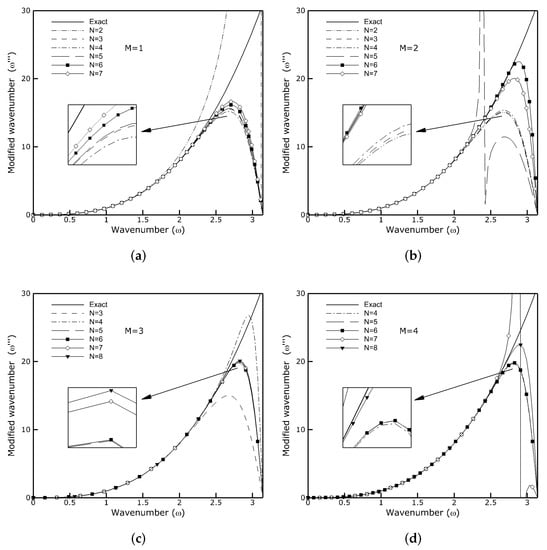
Figure 1. Modified wave number of the 3rd derivative approximation for various CD schemes. (a) $M=1$ and different N, (b) $M=2$ and different N, (c) $M=3$ and different N, (d) $M=4$ and different N.

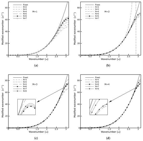
Figure 2. Modified wave number of the 4th derivative approximation for various CD schemes. (a) $M=1$ and different N, (b) $M=2$ and different N, (c) $M=3$ and different N, (d) $M=4$ and different N.

2.3. Test Computations

As a test example showing the accuracy of the approximation of derivatives using the high-order CD schemes, we introduce the function $u(x,t)$ depending on the spatial and temporal coordinate:

$$u(x,t)={cos}^2\left(x\right)sin\left(3x\right)+sin(x-4t-2)$$

(13)

This function will be later used in Section 3.5 as an analytical solution of the 5th-order KdV equation. At the moment, the time coordinate in (13) is set to zero ($t=0$), as we only analyze the accuracy of the spatial derivative approximation. Figure 3 shows a comparison of the numerically and analytically computed first five derivatives of the function (13) using the CD scheme with $M=1$ and $N=7$ on the mesh consisting of $K=257$ nodes. It can be seen that the lines and symbols overlap almost perfectly. The solution errors of the approximated derivative calculated based on the results obtained by applying CD schemes with $M=1$ and various N are shown in Figure 4. The bold lines indicate the expected theoretical orders of approximation, while the dashed lines, dotted lines, and lines with symbols show the dependence of the solution error on mesh density. Based on these results, the actual orders of particular discretization schemes are calculated from the formula:

$$p=\frac{log({\mathrm{Error}}_1/{\mathrm{Error}}_2)}{log(h_1/h_2)}$$

(14)

where ${\mathrm{Error}}_{1,2}$ are the errors on two successive meshes of which the node spacings are $h_1$ and $h_2$, respectively. These errors are computed as the $L^2$ norm of error defined as:

$$L_{Error}^2=\sqrt{\frac{1}{K}\sum _{i=1}^K{[u^{\left(r\right)}\left(x_i\right)-u^{(r,a)}\left(x_i\right)]}^2}$$

(15)

where $u^{\left(r\right)}\left(x_i\right)$ and $u^{(r,a)}\left(x_i\right)$ are the approximate and analytical values of the r-th derivative at the $x_i$ mesh node. Note that all the results presented in this paper were obtained using a 64-bit precision Fortran code with the real numbers declared by the parameter kind=selected_real_kind(15,307). The test calculations have been performed on a series of meshes consisting of up to $K=257$ nodes. It can be seen that in all cases, the obtained orders of approximation agree very well with the theoretical ones. It is worth noting that for large N values, e.g., $N=11,13$, the error drops to very low values already on coarse meshes. Moreover, only in the case of the 1st derivative approximation, it reaches the machine precision accuracy (15 significant digits). In the remaining cases, the solutions seem to be pronouncedly contaminated by the round-off error. It can be seen that the importance of this factor increases with the order of the approximated derivative.

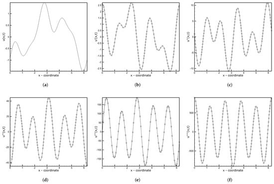
Figure 3. Test function $u(x,t)$ and its analytical (solid lines) and approximated (symbols) derivatives obtained using the CD scheme with $M=1$ and $N=7$. (a) Test function, (b) 1st derivative, (c) 2nd derivative, (d) 3rd derivative, (e) 4th derivative, (f) 5th derivative.

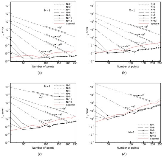
Figure 4. Solution errors of reconstructed derivatives calculated based on the results obtained applying CD schemes with $M=1$ and various N. (a) 1st derivative, (b) 2nd derivative, (c) 3rd derivative, (d) 5th derivative.

Furthermore, it is seen that the round-off error plays a more important role when the number of mesh points increases, and it causes the growth of the solution error. However, this is expected as the contribution of the round-off error to the overall error is dependent on the number of arithmetic operations (additions, multiplications, etc.), of which there are more in dense meshes. Additionally, in Figure 4, we show the error lines of the derivative approximations obtained by applying the Fourier approximation method [54] (red lines). In general, the Fourier approximation is regarded as the most accurate among all discretization methods. If the computational mesh is capable of capturing all scales, it provides an analytical solution. This is the case that we are considering here, and, as one could expect, the error in approximating derivatives by the Fourier method is already at the machine precision level on the coarsest mesh. Intriguing is that the Fourier approximation is more sensible to the round-off error than the CD schemes. Partially, it may depend on how the approximation formulas are implemented in a numerical code [55], but this issue is left for future studies.

3. Results

In this section, we apply CD schemes to solve the linear dispersive wave (LdW) equation, the Korteweg–de Vries (KdV)-like equations, and the Kuramoto–Sivashinsky (KS) equation. These are time-dependent equations and the time integration is performed using the classical explicit fourth-order Runge–Kutta method with the time-step $\mathsf{\Delta }t={10}^{-6}$, for which the obtained solutions are practically independent of time discretization errors, as found in preliminary tests. The only exception is the test case analyzed in Section 3.5, where the time-step was shortened for accuracy and stability reasons, as will be discussed there.

3.1. Third-Order Linear Dispersive Wave (LdW) Equation

The third-order LdW equation can be considered as a linearized form of the KdV equation analyzed in the next section. It is defined as:

$$u_t+c^{-2}{u}_{xxx}=0.$$

(16)

For the initial condition $u(x,0)=sin\left(cx\right)$ and the periodic boundary conditions in the domain $x\in [0,2\pi ]$, the exact solution is $u(x,t)=sin\left(c\right(x+t\left)\right)$. The solution to the Equation (16) is a wave that moves to the left along the ‘x’-direction. Li et al. [34] solved (16) with $c=1$ and $c=8$ using 4th and 6th-order FD and CD schemes. They showed better performance of the CD schemes than the FD schemes of the same order. Here, we solve (16) with the parameter $c=1,8,$ and 16 on the meshes consisting of $K=33,49,65,\dots ,257$ nodes in the time span $t\in [0,1]$. Note that increasing the c parameter increases the frequency of the analytical solution, both in time and space (see Figure 5), and this makes the solution of (16) more difficult compared to what has been done in [34]. The computations are performed using CD schemes with $M=1-4$ and various N up to the 32nd order. Figure 5 shows the numerical solutions obtained on the mesh with $K=257$ nodes for the CD scheme of the 26th order with $M=1$ and $N=13$ for various c. The grey lines indicate the local solution error. As can be seen, the agreement with the analytical solution is excellent. The calculated errors for the schemes with $M=1$ and different N, depending on the parameter c, are presented in Figure 6. The error is computed in the same way as in (15) with the derivatives replaced by the function values. It can be seen that for $c=1$ for all M and N combinations, the error is already very small on coarse meshes and the increase of the mesh points does not improve the solution accuracy, i.e., the error stagnates at the level $\mathcal{O}\left({10}^{-10}\right)$. For $c=8$ and $c=16$, the situation is different, i.e., when the number of nodes increases, the errors almost linearly drop from the initial levels. The slopes of the error lines are in good agreement with the expected orders of approximations. Ultimately, for dense meshes, the errors remain on the same level as for $c=1$, but for $c=8$ and $c=16$, this starts from a different number of the mesh point K. Moreover, it can be seen that using a more accurate scheme (larger N) speeds up the achievement of the minimum error. It is worth noting that its level corresponds well to the minimum error rate calculated for the 3rd derivative approximation in Section 2.3 (see Figure 4). Here, however, it does not increase with K, which may be due to either the dissipative character of the Runge–Kutta method or a different analytical solution. The error lines for the case with $c=16$ computed using CD schemes with various M and N combinations are shown in Figure 7. It can be seen that the expected error behavior indicated by the straight reference lines is reached in all the cases. Additionally, one can observe that CD schemes of the same order, i.e., the same $(M+N)$, are more accurate when the M values are larger. For instance, the combinations $M=1$, $N=7$ and $M=2$, $N=6$, and $M=3$, $N=5$ as well as $M=4$, $N=4$ all resulted in the discretization scheme of the 14th order. Table 1 shows the exact error values of particular CD schemes. It can be seen that the schemes with a larger M are generally more accurate. As mentioned in Section 2.1, this is due to the differences in the leading terms of the truncation errors. Hence, one can conclude that having a given computational stencil ($M+N$), it is better to choose the scheme with a larger M. It is worth noting that only the schemes with $M=1,N=7$ and $M=2,N=6$ approach the 14th-order accuracy, but do not reach it exactly. This may be due to an accumulation or interaction of the leading terms of the truncation errors. On the other hand, these mutual error interactions seem to have a positive impact on the solutions obtained using $M=3,N=5$ and $M=4,N=4$, since in these cases, the calculated order of approximation is higher than theoretically expected.

Figure 5. LdW equation: the analytical and numerical solutions obtained on the mesh with $K=257$ nodes. (a) $c=1$ in (16), (b) $c=8$ in (16), (c) $c=16$ in (16).

Figure 6. LdW equation: the solution errors calculated based on the results obtained applying CD schemes with $M=1$ and various N. (a) $c=1$ in (16), (b) $c=8$ in (16), (c) $c=16$ in (16).

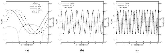
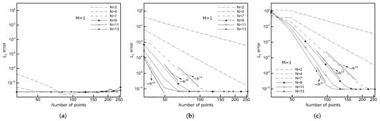
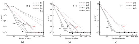
Figure 7. Linear dispersive wave equation ($c=16$): the solution errors calculated based on the results obtained applying CD schemes with various combinations of the computational stencils M and N. (a) $M=2$ and various N, (b) $M=3$ and various N, (c) $M=4$ and various N.

Table 1. Calculated error values and orders (p) of the CD schemes with equal $(M+N)$.

	M = 1, N = 7		M = 2, N = 6		M = 3, N = 5		M = 4, N = 4
Grid	r	p	Error	p	Error	p	Error	p
33	$3.09\times {10}^{-1}$	-	$8.54\times {10}^{-1}$	-	$1.36\times {10}^0$	-	$1.35\times {10}^0$	-
49	$3.64\times {10}^{-2}$	$5.41$	$3.88\times {10}^{-3}$	$13.6$	$1.50\times {10}^{-3}$	$17.2$	$1.78\times {10}^{-3}$	$16.7$
65	$7.89\times {10}^{-4}$	$13.6$	$6.33\times {10}^{-5}$	$14.6$	$8.33\times {10}^{-6}$	$18.3$	$1.20\times {10}^{-5}$	$17.6$
81	$3.97\times {10}^{-5}$	$13.6$	$2.68\times {10}^{-6}$	$14.4$	$1.87\times {10}^{-7}$	$17.2$	$3.32\times {10}^{-7}$	$16.3$
97	$3.38\times {10}^{-6}$	$13.7$	$2.06\times {10}^{-7}$	$14.2$	$9.29\times {10}^{-9}$	$16.7$	$2.00\times {10}^{-8}$	$15.5$
113	$4.14\times {10}^{-7}$	$13.7$	$2.36\times {10}^{-8}$	$14.2$	$8.40\times {10}^{-10}$	$15.7$	$2.04\times {10}^{-9}$	$14.9$
129	$6.66\times {10}^{-8}$	$13.7$	$3.57\times {10}^{-9}$	$14.3$	$1.77\times {10}^{-10}$	$11.7$	$3.60\times {10}^{-10}$	$13.1$
145	$1.32\times {10}^{-8}$	$13.7$	$6.16\times {10}^{-10}$	$15.0$	$1.03\times {10}^{-10}$	$4.64$	$1.38\times {10}^{-10}$	$8.22$
161	$3.17\times {10}^{-9}$	$13.7$	$7.24\times {10}^{-11}$	$20.4$	$9.21\times {10}^{-11}$	$1.07$	$1.00\times {10}^{-10}$	$3.07$
177	$9.17\times {10}^{-10}$	$13.1$	$4.68\times {10}^{-11}$	$4.6$	$9.01\times {10}^{-11}$	$0.23$	$9.21\times {10}^{-11}$	$0.86$
193	$3.37\times {10}^{-10}$	$11.5$	$7.69\times {10}^{-11}$	$-5.73$	$8.97\times {10}^{-11}$	$0.05$	$9.22\times {10}^{-11}$	$0.24$
209	$1.71\times {10}^{-10}$	$8.52$	$8.54\times {10}^{-11}$	$-1.32$	$8.96\times {10}^{-11}$	$0.02$	$8.98\times {10}^{-11}$	$0.07$
225	$1.18\times {10}^{-10}$	$4.96$	$8.81\times {10}^{-11}$	$-0.41$	$8.95\times {10}^{-11}$	$0.00$	$8.96\times {10}^{-11}$	$0.02$
241	$1.00\times {10}^{-10}$	$2.40$	$8.90\times {10}^{-11}$	$-0.14$	$8.95\times {10}^{-11}$	$0.00$	$8.96\times {10}^{-11}$	$0.01$
257	$9.41\times {10}^{-11}$	$1.05$	$8.93\times {10}^{-11}$	$-0.05$	$8.95\times {10}^{-11}$	$0.00$	$8.96\times {10}^{-11}$	$0.00$

3.2. Third-Order Korteweg–de Vries (KdV) Equation

In the literature, one can find various forms of the KdV equation. Recently, Benia and Scapellato [56] presented an analysis of the existence and uniqueness of a solution to the third-order non-linear KdV equation. Here, we consider it in a typical form, very similar to the one studied in [56], given as:

$$u_t-3{\left(u^2\right)}_x+u_{xxx}=0.$$

(17)

For the initial condition $u(x,0)=-2{\mathrm{sech}}^2\left(x\right)$, the exact solution of (17) is $u(x,t)=-2{\mathrm{sech}}^2(x-4t)$. One should mention that this problem was investigated by Li et al. [34], who solved it using the 6th-order CD scheme with and without the 10th-order low-pass filter. Their results were comparable to Yan and Shu [35] solutions obtained with the help of the LGD method. Here, we solve Equation (17) using the previously discussed CD schemes on the meshes consisting of $K=33,49,65,\dots ,257$ nodes over the time period $t\in [0,0.5]$ in the periodic domain $x\in [-10,10]$. An important remark that should be made at this point is that the solution of (17) is not periodic in physical space. Its period is imaginary and equals to $i\pi$, where $i=\sqrt{-1}$. The consequences of the assumed periodicity are discussed later. Figure 8a shows the numerical and analytical solution at $t=0,0.25,0.5$ on the mesh consisting of $K=257$ points. It shows how the initial function moves along the ‘x’-coordinate. Ideally, as the KdV Equation (17) does not include a dissipative term, the initial shape of the function should be preserved over the entire simulation time and only shifted to the right side. Figure 8b,c show the $L^2$ norm of the errors computed based on the results obtained by applying various combinations of M and N. As in the case of the LdW equation, the agreement is very good. It can be seen that for $(M+N)\ge 10$, the errors are almost equal and this means that a further increase of the approximation order would not increase the solution accuracy. One should also note that the minimum error level reached $\mathcal{O}\left({10}^{-7}\right)$ is significantly higher than during the solution of the LdW equation and higher than one could predict based on the accuracy of the 3rd derivative approximation (see Section 2.3, Figure 4). The reason for such behavior is the lack of periodicity of the analytical solution in the real space, as mentioned above. Looking at the solution behavior in Figure 8a, one can readily notice that as time passes, the peak of the function $u(x,t)$ approaches the boundary at $x=10$ at which neither the function itself nor their derivative is periodic. In such a case, the errors of the derivative approximations are overwhelmed by the errors stemming from the violation of the periodicity conditions. The obtained results show that they are at the level $\mathcal{O}\left({10}^{-7}\right)$. This prevents both from obtaining the solution with the expected order of accuracy (e.g., 22nd for $M=3,N=9$) and reducing the overall solution error to the values below $\mathcal{O}\left({10}^{-7}\right)$.

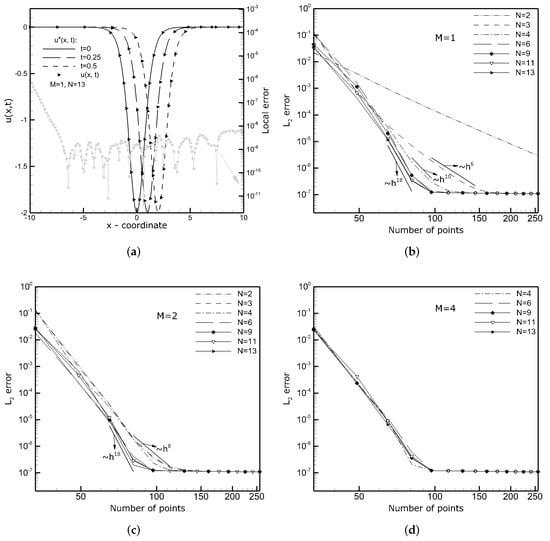
Figure 8. Third-order KdV equation: the exact and numerical solutions at the selected time instances with the grey line representing the local error at $t=0.5$ (a), the overall solution errors (b–d) for various combinations of M and N. (a) Exact (lines) and numerical (symbols) solutions, (b) $M=1$ and various N, (c) $M=2$ and various N, (d) $M=4$ and various N.

3.3. Fourth-Order Kuramoto–Sivashinsky (KS) Equation

The Kuramoto–Sivashinsky (KS) equation is a model of diffusion instabilities in a laminar flame front. It is defined as:

$$u_t+u{u}_x+u_{xx}+\sigma u_{xxx}+u_{xxxx}=0.$$

(18)

For the initial condition:

$$u(x,0)=c+9-15(tanh\left(k(x-x_0)\right)+{tanh}^2\left(k(x-x_0)\right)-{tanh}^3\left(k(x-x_0)\right))$$

(19)

its exact solution is given as:

$$u(x,t)=c+9-15(tanh\left(k(x-ct-x_0)\right)+{tanh}^2\left(k(x-ct-x_0)\right)-{tanh}^3\left(k(x-ct-x_0)\right)).$$

(20)

Following Xu et al. [57], who solved Equation (18) using the LDG method, we set $c=6$, $\sigma =4$, $k=0.5$, and $x_0=-10$. Similarly, as in the 3rd-order KdV equation, the solution of the KS equation is the wave traveling along the ‘x’-coordinate and has the form of a solitary wave. Thus, the solution (20) is not periodic in real space. Its period is imaginary and with the selected coefficients it equals $2i\pi$. Nevertheless, we treat the problem (18) as periodic along the ‘x’-coordinate. To minimize the impact of the errors due to the lack of the real periodicity, which will be revealed in a long-lasting simulation ($t=4$), we assume a large computational domain $x\in [-30,30]$. Figure 9a shows the analytical and numerical solution of (18) obtained on the mesh with $K=257$ nodes at time $t=0.0,2.0,4.0$ using the CD scheme with $M=1$ and $N=13$. The dependence of the solution errors on the mesh density for various M and N combinations at time $t=4.0$ is presented in Figure 9b–d. It can be seen that for large $M+N$ values, the error lines do not show the improvement of the solution accuracy and for the meshes with $K>161$, the errors remain on the same constant level $\mathcal{O}\left({10}^{-7}\right)$. However, the presented results are an order of accuracy better than the best solution obtained in [57] using the LDG method. On a very dense mesh ($K=320$), and at an early simulation time ($t=1.0$), the error obtained was one order of magnitude higher ($2.75\times {10}^{-6}$) than found here already on the twice coarser mesh.

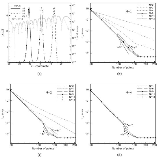
Figure 9. Kuramoto–Sivashinsky equation: the solution errors calculated based on the results obtained applying CD schemes with various combinations of the computational stencils M and N. (a) Exact (lines) and numerical (symbols) solutions, (b) $M=1$ and various N, (c) $M=2$ and various N, (d) $M=4$ and various N.

3.4. Fifth-Order Korteweg–de Vries (fKdV) Equations

In this section, we consider the generalized form of the fifth-order KdV (fKdV) equation:

$$u_t+a{u}^2{u}_x+b{u}_x{u}_{xx}+cu{u}_{xxx}+d{u}_{xxxxx}=0$$

(21)

where a, b, c, and d are constants. Two types of the fKdV equation, which have a remarkable importance in the description of wave phenomena are the Sawada–Kotera (SK) equation [58] with the coefficients $a=45$, $b=15$, $c=15$, and $d=1$, and the Lax equation [59,60], with $a=30$, $b=30$, $c=10$, and $d=1$. The analytical solutions of the SK and Lax equations have the form of the traveling wave. For the initial condition $u(x,0)=2k^2{\mathrm{sech}}^2\left[k(x-c)\right]$, the analytical solution of the SK equation is $u(x,t)=2k^2{\mathrm{sech}}^2\left[k(x-16k^{4}t-c)\right]$, and the one of the Lax equation with the initial condition $u(x,0)=2k^2[2-3{tanh}^2\left(k(x-c)\right)]$ is given by $u(x,t)=2k^2[2-3{tanh}^2\left(k(x-56k^{4}t-c)\right)]$. In this paper, we consider the SK and Lax equations with the coefficients $k=0.01$ and $c=0.0$, as used in Bakodah [61] and Ahmad et al. [62]. These authors applied rather very complex methods, i.e., the modified Adomian decomposition method and the modified variational iteration algorithm-II, but obtained very accurate results. With the above values of k and c, the period of the solution, although imaginary, was very large ($100i\pi$), but more importantly, the solution at small times moved only slightly from its initial position, with the peak value centered at $x=0.0$. Figure 10a shows the analytical and numerical solutions of the SK and Lax equations on the mesh consisting of $K=257$ points obtained using the 6th-order CD scheme ($M=1$, $N=4$) at time $t=1.0$, at which we analyze the solution accuracy, and, for comparison, at time $t=50\times {10}^6$ (dashed lines). The fact that the peak at $t=1.0$ stays far from the boundary means that the lack of periodicity in real space should not have a significant destructive impact on the solution accuracy. Indeed, the solution error reached the machine precision, i.e., it dropped to $1.45\times {10}^{-14}$ for the SK equation and $6.37\times {10}^{-13}$ for the Lax equation.

Figure 10. fKdV equations: the analytical and numerical solutions of the SK and Lax equations obtained on the mesh with $K=257$ nodes (a), the source term in the modified Lax Equation (22) (b). (a) The solutions of the SK and Lax equations, (b) the source term (23).

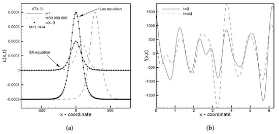
3.5. Fifth-Order Korteweg–de Vries (fKdV) Equation with a Manufactured Solution

In the last section, we analyze the accuracy of the solution of a modified Equation (21) of which the analytical solution is periodic in real space in the domain $x\in [0,2\pi ]$. To do that, we assumed the analytical solution as the function defined in (13) of which substitution to (21) along with the coefficients corresponding to the Lax equation, transformed it into:

$$u_t+30u^2{u}_x+30u_x{u}_{xx}+10u{u}_{xxx}+u_{xxxxx}=f(x,t)$$

(22)

where the source term on the right side is defined as:

$$\begin{array}{cc}\hfill f(x,t)=& -3cos\left(k\right)+30{[R_1-sin\left(k\right)]}^2[-2R_2+3R_3+cos\left(k\right)]\hfill \\ & +30[-2R_2+3R_3+cos\left(k\right)][2R_4-12R_5-11R_1+sin\left(k\right)]\hfill \\ & +10[R_1-sin\left(k\right)][62R_2+18R_6-45R_3-cos\left(k\right)]-1562R_2-660R_6+903R_3\hfill \end{array}$$

(23)

where:

$$\begin{array}{cc}\hfill & k=-x+4t+2,\hfill \\ \hfill & R_1=cos{\left(x\right)}^{2}sin\left(3x\right),R_2=cos\left(x\right)sin\left(3x\right)sin\left(x\right),R_3=cos{\left(x\right)}^{2}cos\left(3x\right),\hfill \\ \hfill & R_4=sin{\left(x\right)}^{2}sin\left(3x\right),R_5=cos\left(x\right)cos\left(3x\right)sin\left(x\right),R_6=sin{\left(x\right)}^{2}cos\left(3x\right)\hfill \end{array}$$

(24)

This source term ensures that the function (13) is the solution to the Equation (22). Its spatial variation at the initial time $t=0.0$ and time $t=\pi /4$ is shown in Figure 10b. In the present test case, to verify how the solution behaves starting from different initial conditions, we set the initial times $t_0$ to $0.0$, $\frac{\pi }{8}$, $\frac{\pi }{4}$, $\frac{\pi }{3}$, $\frac{3\pi }{8}$, $\frac{\pi }{2}$, and run the computations for $t={10}^{-6}$. Due to the very large magnitude of the source term (see Figure 10b), the time-step was reduced to $\mathsf{\Delta }t={10}^{-8}$ for stability reasons and to eliminate the dependence of the solution on the time discretization error. Figure 11 presents the analytical and numerical solutions of the KdV Equation (22) using the 26th-order CD scheme on the mesh consisting of $K=257$ nodes for the time $t_0+{10}^{-5}$. It can be seen that the agreement with the analytical solution was very good. The exact values of the solution errors calculated based on the results obtained using different combinations of M and N in CD schemes on the mesh consisting of $K=257$ nodes are shown in Table 2. As can be seen, the CD schemes provide very good accuracy in all cases, with an error at the level limited by the accuracy of the 5th-order derivative approximation, which can be deduced from the solutions presented in Figure 4.

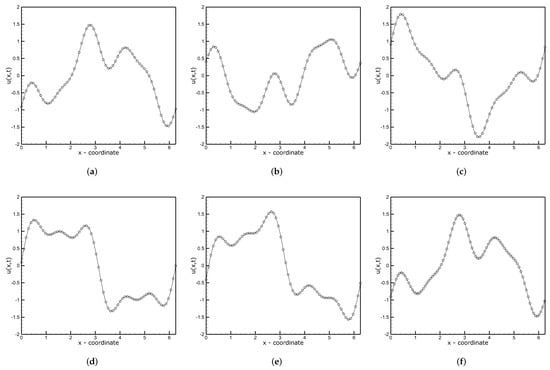
Figure 11. fKdV equation: the analytical (solid lines) and numerical (symbols) solutions obtained on the mesh with $K=257$ nodes in the following moments of time: 0, $\frac{\pi }{8}$, $\frac{\pi }{4}$, $\frac{\pi }{3}$, $\frac{3\pi }{8}$, $\frac{\pi }{2}$. (a) $t=0$, (b) $t=\frac{\pi }{8}$, (c) $t=\frac{\pi }{4}$, (d) $t=\frac{\pi }{3}$, (e) $t=\frac{3\pi }{8}$, (f) $t=\frac{\pi }{2}$.

Table 2. Calculated error values for CD schemes with equal $(M+N)$.

Time	M = 1, N = 7	M = 2, N = 6	M = 3, N = 5	M = 4, N = 4
0	$2.70\times {10}^{-13}$	$7.41\times {10}^{-13}$	$3.69\times {10}^{-13}$	$2.95\times {10}^{-13}$
$\frac{\pi }{8}$	$6.26\times {10}^{-11}$	$6.26\times {10}^{-11}$	$6.26\times {10}^{-11}$	$6.25\times {10}^{-11}$
$\frac{\pi }{4}$	$6.26\times {10}^{-11}$	$6.24\times {10}^{-11}$	$6.25\times {10}^{-11}$	$6.26\times {10}^{-11}$
$\frac{\pi }{3}$	$2.51\times {10}^{-10}$	$2.52\times {10}^{-10}$	$2.52\times {10}^{-10}$	$2.51\times {10}^{-10}$
$\frac{3\pi }{8}$	$2.51\times {10}^{-10}$	$2.51\times {10}^{-10}$	$2.51\times {10}^{-10}$	$2.51\times {10}^{-10}$
$\frac{\pi }{2}$	$2.51\times {10}^{-10}$	$2.51\times {10}^{-10}$	$2.51\times {10}^{-10}$	$2.51\times {10}^{-10}$

4. Conclusions

This paper presents a detailed analysis of very high-order compact difference (CD) schemes and their accuracy when applied to solving linear and non-linear high-order partial differential equations (PDEs). The compact form of derived CD schemes for odd and even derivatives allows an easy formulation of the discretization formulas of the 20th or 30th order. Both the analysis of the truncation errors and the analysis in the Fourier space showed that the proposed CD schemes approach spectral accuracy in terms of the ability to resolve small-scale phenomena. The test cases included both a simple verification of the CD formulas based on the approximation of derivatives of a test function and classical problems describing important physical phenomena (wave transport, dispersion, or instability of laminar flame front), i.e., the 3rd-order linear dispersive wave equation, 3rd and 5th-order Korteweg–de Vries-like equations, and 4th-order Kuramoto–Sivashinsky equation. Comprehensive analysis showed that the obtained solutions reach the expected accuracy with the orders of the schemes in good accordance with the theoretical ones. However, it has been shown that in some cases, the increase of the computational stencil on which the CD schemes operate, and thus the increase of the approximation order, does not bring real benefits. This is because of either reaching the machine precision already on relatively coarse computational meshes or due to the round-off errors. For the CD schemes of the 16th order or higher, both factors turned out to have a decisive impact on the reduction of the solution error, with the increase in the number of nodes in the computational meshes.

References

- Kajishima, T.; Taira, K. Computational Fluid Dynamics: Incompressible Turbulent Flows; Springer International Publishing: Berlin/Heidelberg, Germany, 2017. [Google Scholar]
- Boutayeb, A.; Chetouani, A. A mini-review of numerical methods for high-order problems. Int. J. Comput. Math. 2007, 84, 563–579. [Google Scholar] [CrossRef]
- Lele, S.K. Compact finite difference schemes with spectral-like resolution. J. Comput. Phys. 1992, 103, 16–42. [Google Scholar] [CrossRef]
- Gamet, L.; Ducros, F.; Nicoud, F.; Poinsot, T. Compact finite difference schemes on non-uniform meshes. Application to direct numerical simulations of compressible flows. Int. J. Numer. Methods Fluids 1999, 29, 159–191. [Google Scholar] [CrossRef]
- Boersma, B.J. A staggered compact finite difference formulation for the compressible Navier–Stokes equations. J. Comput. Phys. 2005, 208, 675–690. [Google Scholar] [CrossRef]
- Tyliszczak, A. A high-order compact difference algorithm for half-staggered grids for laminar and turbulent incompressible flows. J. Comput. Phys. 2014, 276, 438–467. [Google Scholar] [CrossRef]
- San, O.; Staples, A.E. High-order methods for decaying two-dimensional homogeneous isotropic turbulence. Comput. Fluids 2012, 63, 105–127. [Google Scholar] [CrossRef]
- San, O. A dynamic eddy-viscosity closure model for large eddy simulations of two-dimensional decaying turbulence. Int. J. Comput. Fluid Dyn. 2014, 28, 363–382. [Google Scholar] [CrossRef]
- Ekaterinaris, J.A. Implicit, High-Resolution, Compact Schemes for Gas Dynamics and Aeroacoustics. J. Comput. Phys. 1999, 156, 272–299. [Google Scholar] [CrossRef]
- Lee, D.-J.; Lee, I.C.; Kim, J.W.; Kim, Y.N. Computational aeroacoustics (CAA) Flow-Acoustic Feedback Problems. In Proceedings of the Conference: 6th KSME-JSME Thermal and Fluids Engineering Conference (TFEC6), Jeju, Korea, 20–23 March 2005. [Google Scholar]
- Zuo, Z.; Maekawa, H. Application of a High-Resolution Compact Finite Difference Method to Computational Aeroacoustics of Compressible Flows. In Proceedings of the ASME-JSME-KSME 2011 Joint Fluids Engineering Conference: Volume 1, Symposia—Parts A, B, C, and D, Hamamatsu, Japan, 24–29 July 2011. [Google Scholar]
- Tyliszczak, A. LES–CMC study of an excited hydrogen flame. Combust. Flame 2015, 162, 3864–3883. [Google Scholar] [CrossRef]
- Tyliszczak, A. High-order compact difference algorithm on half-staggered meshes for low Mach number flows. Comput. Fluids 2016, 127, 131–145. [Google Scholar] [CrossRef]
- Wawrzak, A.; Tyliszczak, A. Implicit LES study of spark parameters impact on ignition in a temporally evolving mixing layer between H2/N2 mixture and air. Int. J. Hydrogen Energy 2018, 43, 9815–9828. [Google Scholar] [CrossRef]
- Visbal, M.R.; Gaitonde, D.V. High-Order-Accurate Methods for Complex Unsteady Subsonic Flows. AIAA J. 1999, 37, 1231–1239. [Google Scholar] [CrossRef]
- Visbal, M.R.; Gaitonde, D.V. Very High-Order Spatially Implicit Schemes For Computational Acoustics On Curvilinear Meshes. J. Comput. Acoust. 2001, 9, 1259–1286. [Google Scholar] [CrossRef]
- Wang, Z.; Li, J.; Wang, B.; Xu, Y.; Chen, X. A new central compact finite difference scheme with high spectral resolution for acoustic wave equation. J. Comput. Phys. 2018, 366, 191–206. [Google Scholar] [CrossRef]
- Shang, J.S. High-Order Compact-Difference Schemes for Time-Dependent Maxwell Equations. J. Comput. Phys. 1999, 153, 312–333. [Google Scholar] [CrossRef]
- Hesthaven, J.S. High-order accurate methods in time-domain computational electromagnetics: A review. Adv. Imaging Electron Phys. 2003, 127, 59–123. [Google Scholar]
- Korteweg, D.J.; de Vries, G. On the change of form of long waves advancing in a rectangular canal, and on a new type of long stationary waves. Philos. Mag. 1895, 39, 422–443. [Google Scholar] [CrossRef]
- Boussinesq, J. Essai sur la Theorie des eaux Courantes Memoires Presentes par Divers Savants; Memoires Presentes par Divers Savants a l’Academie des Sciences de l’Institut National de France; Institut de France: Paris, France, 1877. [Google Scholar]
- Dai, H.-H. Exact Solutions of a Variable-Coefficient KdV Equation Arising in a Shallow Water. J. Phys. Soc. Jpn. 1999, 68, 1854–1858. [Google Scholar] [CrossRef]
- Costa, A.; Osborne, A.R.; Resio, D.T.; Alessio, S.; Chrivì, E.; Saggese, E.; Bellomo, K.; Long, C.E. Soliton Turbulence in Shallow Water Ocean Surface Waves. Phys. Rev. Lett. 2014, 113, 108501. [Google Scholar] [CrossRef]
- Aljahdaly, N.H.; Seadawy, A.R.; Albarakati, W.A. Analytical wave solution for the generalized nonlinear seventh-order KdV dynamical equations arising in shallow water waves. Mod. Phys. Lett. B 2020, 34, 2050279. [Google Scholar] [CrossRef]
- Hunter, J.K.; Vanden-Broeck, J.-M. Solitary and periodic gravity—Capillary waves of finite amplitude. J. Fluid Mech. 1983, 134, 205. [Google Scholar] [CrossRef]
- Milewski, P.A. Three-dimensional localized solitary gravity-capillary waves. Commun. Math. Sci. 2005, 3, 89–99. [Google Scholar] [CrossRef]
- Biswas, H.A.; Rahman, A.; Das, T. An Investigation on Fiber Optical Soliton in Mathematical Physics and Its Application in Communication Engineering. Int. J. Res. Rev. Appl. Sci. 2011, 6, 268–276. [Google Scholar]
- Obregon, M.; Stepanyants, Y. Oblique magneto-acoustic solitons in a rotating plasma. Phys. Lett. A 1998, 249, 315–323. [Google Scholar] [CrossRef]
- Goswami, A.; Singh, J.; Kumar, D. Numerical simulation of fifth order KdV equations occurring in magneto-acoustic waves. Ain Shams Eng. J. 2018, 9, 2265–2273. [Google Scholar] [CrossRef]
- Sahu, B.; Roychoudhury, R. Exact solutions of cylindrical and spherical dust ion acoustic waves. Phys. Plasmas 2003, 10, 4162–4165. [Google Scholar] [CrossRef]
- Guo, M.; Fu, C.; Zhang, Y.; Liu, J.; Yang, H. Study of Ion-Acoustic Solitary Waves in a Magnetized Plasma Using the Three-Dimensional Time-Space Fractional Schamel-KdV Equation. Complexity 2018, 2018, 6852548. [Google Scholar] [CrossRef]
- Grant, A.K.; Rosner, J.L. Supersymmetric quantum mechanics and the Korteweg–de Vries hierarchy. J. Math. Phys. 1994, 35, 2142–2156. [Google Scholar] [CrossRef][Green Version]
- Zakharov, D.V.; Dyachenko, S.A.; Zakharov, V.E. Bounded Solutions of KdV and Non-Periodic One-Gap Potentials in Quantum Mechanics. Lett. Math. Phys. 2016, 106, 731–740. [Google Scholar] [CrossRef]
- Li, J.; Visbal, M.R. High-order Compact Schemes for Nonlinear Dispersive Waves. J. Sci. Comput. 2006, 26, 1–23. [Google Scholar] [CrossRef]
- Yan, J.; Shu, C.-W. A Local Discontinuous Galerkin Method for KdV Type Equations. SIAM J. Numer. Anal. 2002, 40, 769–791. [Google Scholar] [CrossRef]
- Wouwer, A.V.; Saucez, P.; Schiesser, W.E. (Eds.) Adaptive Method of Lines; Chapman and Hall/CRC: Boca Raton, FL, USA, 2001. [Google Scholar]
- Djidjeli, K.; Price, W.G.; Twizell, E.H.; Wang, Y. Numerical methods for the solution of the third- and fifth-order dispersive Korteweg–de Vries equations. J. Comput. Appl. Math. 1995, 58, 307–336. [Google Scholar] [CrossRef]
- Li, J. High-order finite difference schemes for differential equations containing higher derivatives. Appl. Math. Comput. 2005, 171, 1157–1176. [Google Scholar] [CrossRef]
- Yan, J.; Shu, C.-W. Local Discontinuous Galerkin Method for Partial Differential Equations with Higher Order Derivatives. J. Sci. Comput. 2002, 17, 27–47. [Google Scholar] [CrossRef]
- Kuramoto, Y.; Tsuzuki, T. On the Formation of Dissipative Structures in Reaction-Diffusion Systems: Reductive Perturbation Approach. Prog. Theor. Phys. 1975, 54, 687–699. [Google Scholar] [CrossRef]
- Kuramoto, Y.; Tsuzuki, T. Persistent Propagation of Concentration Waves in Dissipative Media Far from Thermal Equilibrium. Prog. Theor. Phys. 1976, 55, 356–369. [Google Scholar] [CrossRef]
- Kuramoto, Y. Diffusion-Induced Chaos in Reaction Systems. Prog. Theor. Phys. Suppl. 1978, 64, 346–367. [Google Scholar] [CrossRef]
- Michelson, D.M.; Sivashinsky, G.I. Nonlinear analysis of hydrodynamic instability in laminar flames—II. Numerical experiments. Acta Astronaut. 1977, 4, 1207–1221. [Google Scholar] [CrossRef]
- Sivashinsky, G.I. Nonlinear analysis of hydrodynamic instability in laminar flames—I. Derivation of basic equations. Acta Astronaut. 1977, 4, 1177–1206. [Google Scholar] [CrossRef]
- Sivashinsky, G.I. On Flame Propagation Under Conditions of Stoichiometry. SIAM J. Appl. Math. 1980, 39, 67–82. [Google Scholar] [CrossRef]
- Chang, H. Evolution on a Falling Film. Annu. Rev. Fluid Mech. 1994, 26, 103–136. [Google Scholar] [CrossRef]
- Chang, H.-C.; Demekhin, E.A. Solitary Wave Formation and Dynamics on Falling Films. Adv. Appl. Mech. 1996, 32, 1–58. [Google Scholar]
- Hooper, A.P.; Grimshaw, R. Nonlinear instability at the interface between two viscous fluids. Phys. Fluids 1985, 28, 37–45. [Google Scholar] [CrossRef]
- Papageorgiou, D.T.; Maldarelli, C.; Rumschitzki, D.S. Nonlinear interfacial stability of core-annular film flows. Phys. Fluids A Fluid Dyn. 1990, 2, 340–352. [Google Scholar] [CrossRef]
- LaQuey, R.E.; Mahajan, S.M.; Rutherford, P.H.; Tang, W.M. Nonlinear Saturation of the Trapped-Ion Mode. Phys. Rev. Lett. 1975, 34, 391–394. [Google Scholar] [CrossRef]
- Carpenter, M.H.; Gottlieb, D.; Abarbanel, S. The stability of numerical boundary treatements for compact high-order finite-difference schemes. J. Comput. Phys. 1993, 108, 272–295. [Google Scholar] [CrossRef]
- Nordström, J.; Mattsson, K.; Swanson, C. Boundary conditions for a divergence free velocity-pressure formulation of the Navier-Stokes equations. J. Comput. Phys. 2007, 225, 874–890. [Google Scholar] [CrossRef]
- Svärd, M.; Nordström, J. Review of summation-by-parts schemes for initial-boundary-value problems. J. Comput. Phys. 2014, 268, 17–38. [Google Scholar] [CrossRef]
- Canuto, C.; Hussaini, M.Y.; Quarteroni, A.; Thomas, A., Jr. Spectral Methods in Fluid Dynamics; Springer Science & Business Media: Berlin/Heidelberg, Germany, 2012. [Google Scholar]
- Bayliss, A.; Class, A.; Matkowsky, B.J. Roundoff Error in Computing Derivatives Using the Chebyshev Differentiation Matrix. J. Comput. Phys. 1995, 116, 380–383. [Google Scholar] [CrossRef]
- Benia, Y.; Scapellato, A. Existence of solution to Korteweg–de Vries equation in a non-parabolic domain. Nonlinear Anal. 2020, 195, 111758. [Google Scholar] [CrossRef]
- Xu, Y.; Shu, C.-W. Local discontinuous Galerkin methods for the Kuramoto–Sivashinsky equations and the Ito-type coupled KdV equations. Comput. Methods Appl. Mech. Eng. 2006, 195, 3430–3447. [Google Scholar] [CrossRef]
- Sawada, K.; Kotera, T. A Method for Finding N-Soliton Solutions of the K.d.V. Equation and K.d.V.-Like Equation. Prog. Theor. Phys. 1974, 51, 1355–1367. [Google Scholar] [CrossRef]
- Lax, P.D. Integrals of nonlinear equations of evolution and solitary waves. Commun. Pure Appl. Math. 1968, 21, 467–490. [Google Scholar] [CrossRef]
- Wazwaz, A.-M. Solitons and periodic solutions for the fifth-order KdV equation. Appl. Math. Lett. 2006, 19, 1162–1167. [Google Scholar] [CrossRef]
- Bakodah, H.O. Modified Adomian Decomposition Method for the Generalized Fifth Order KdV Equations. Am. J. Comput. Math. 2013, 3, 53–58. [Google Scholar] [CrossRef]
- Ahmad, H.; Khan, T.A.; Yao, S.-W. An efficient approach for the numerical solution of fifth-order KdV equations. Open Math. 2020, 18, 738–748. [Google Scholar] [CrossRef]
Publisher’s Note: MDPI stays neutral with regard to jurisdictional claims in published maps and institutional affiliations. |
© 2022 by the authors. Licensee MDPI, Basel, Switzerland. This article is an open access article distributed under the terms and conditions of the Creative Commons Attribution (CC BY) license (https://creativecommons.org/licenses/by/4.0/).