Tracking Dynamic Source Direction with a Novel Stationary Electronic Nose System

Abstract
:1. Introduction
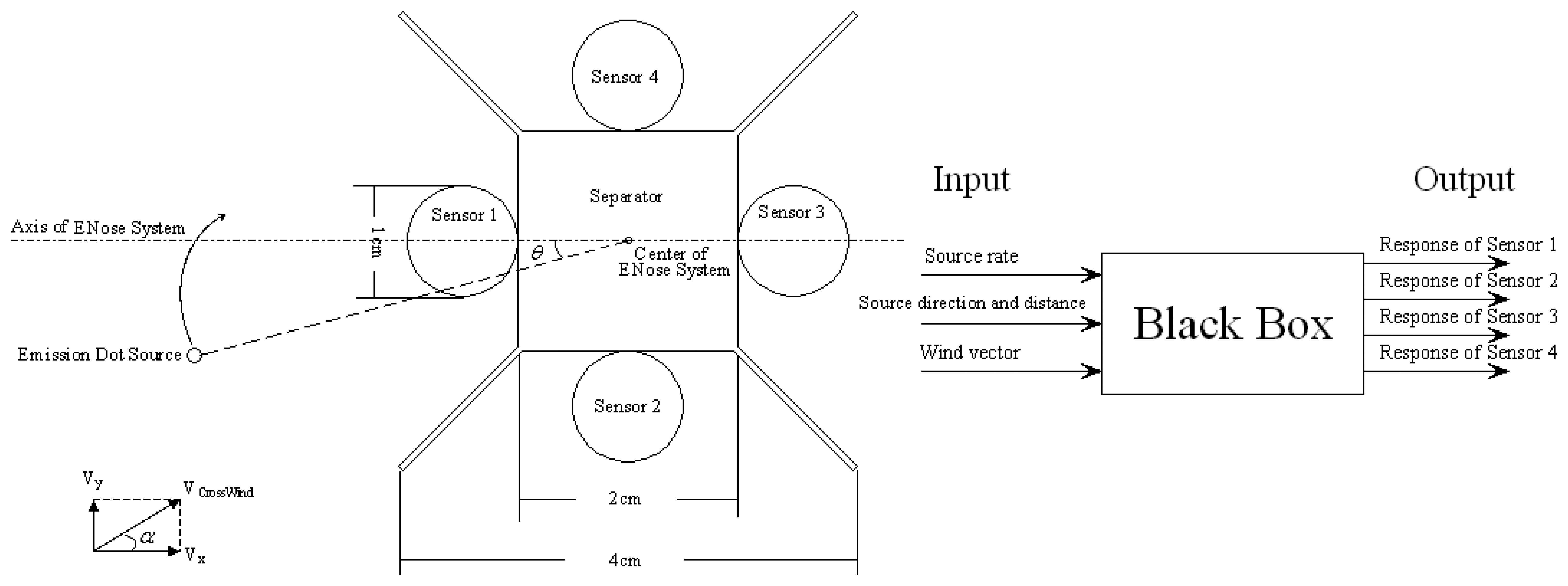
2. System Structure
3. Three-Step Approach to Determine Static Source Direction
- If α<= η, the case is treated as advection;
- If α< η, it is treated as a crosswind;
- If
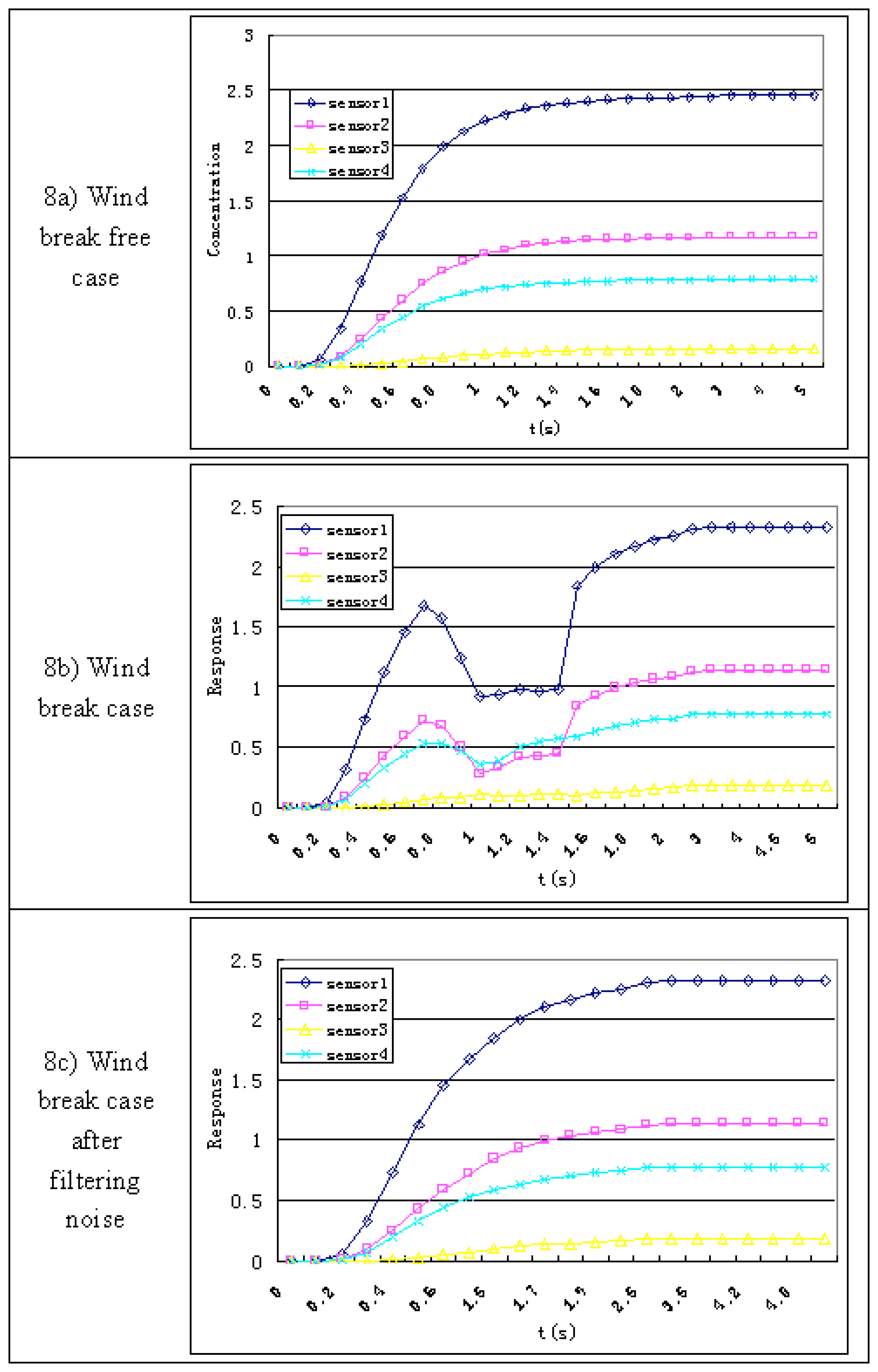
- Vwind(t) = 0, t1 < t < t2
- Vwind(t) = a, t < t1 OR t > t2, where a is non - zero constant,
3.1. Determine the direction of source to center of ENose system in advection case
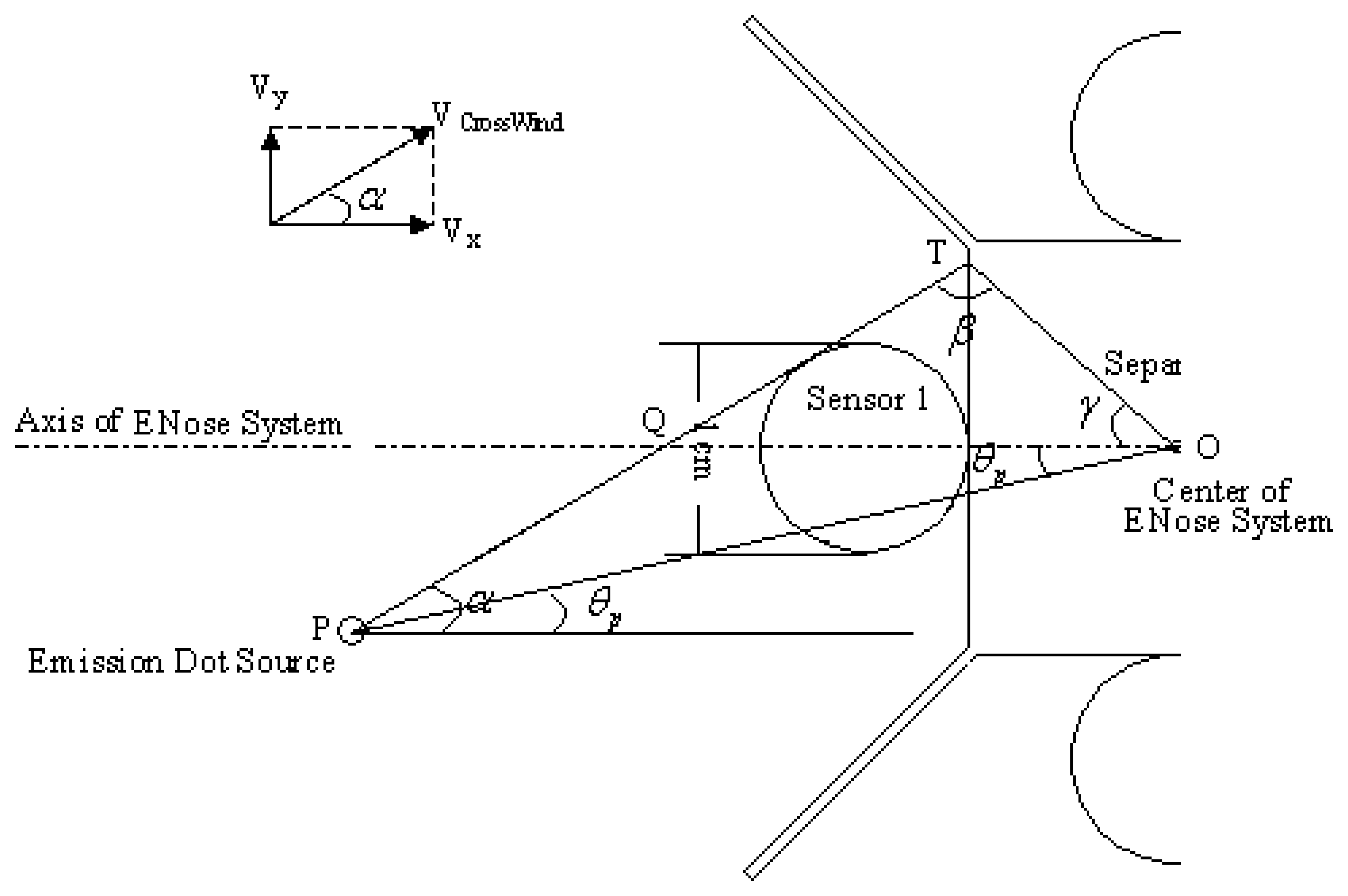
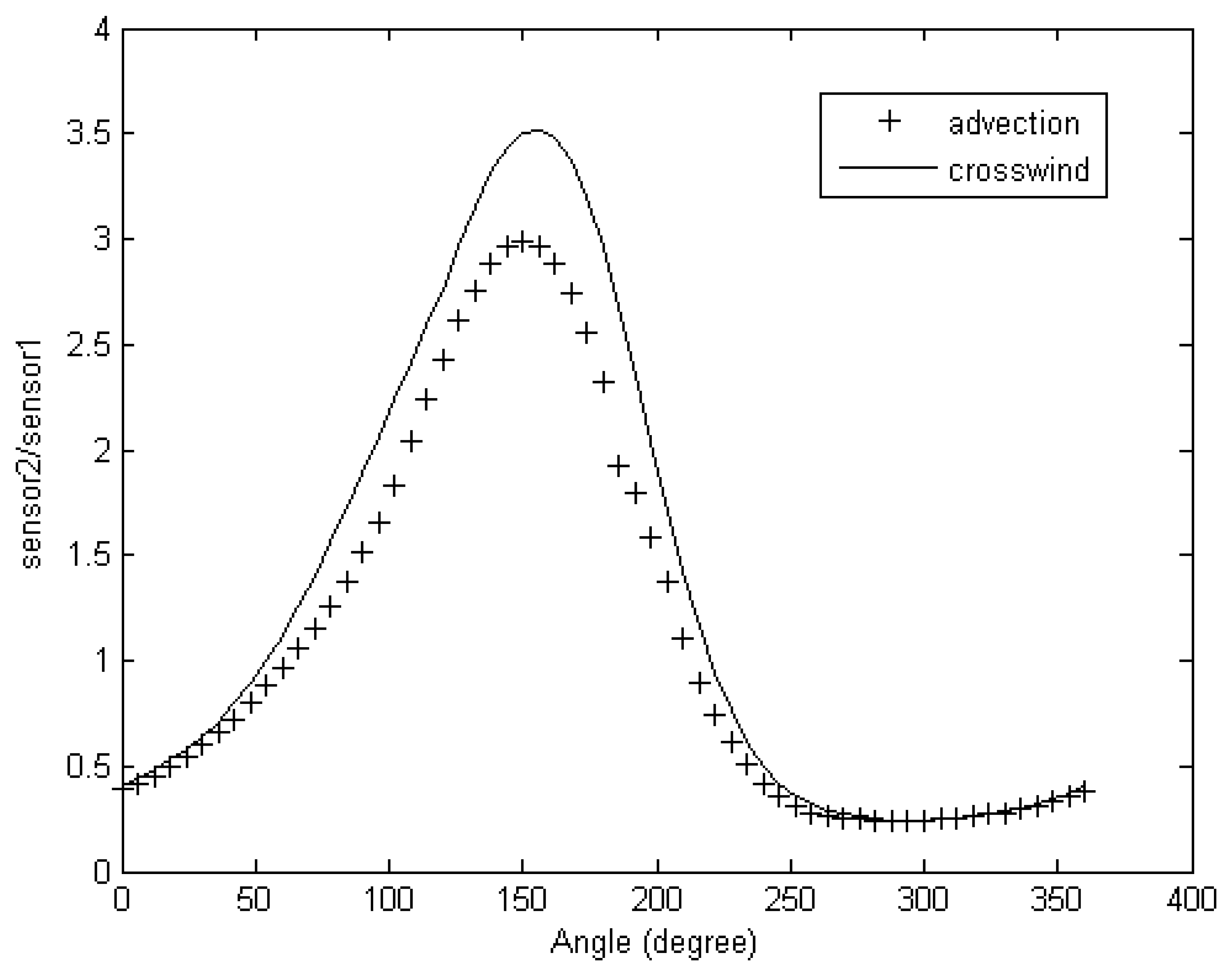
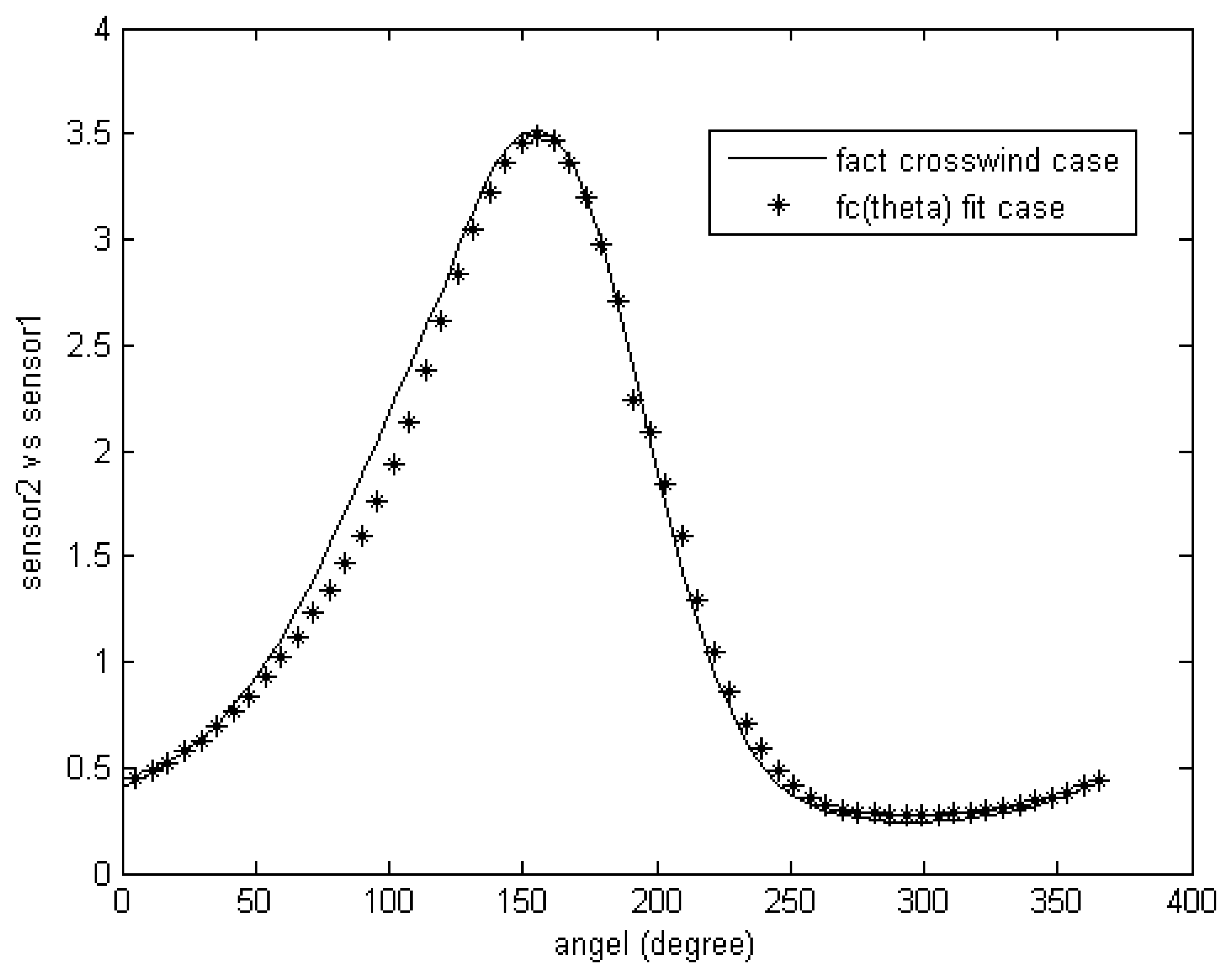
3.2. Crosswind case direction detection
- (1)
- The source position is on a line with slope of crosswind direction α
- (2)
- This line is a tangent of sensor 1.
- SSE -- The sum of squares due to error. This statistic measures the deviation of the responses from the fitted values of the responses. A value closer to 0 indicates a better fit.
- R-square -- The coefficient of multiple determination. This statistic measures how successful the fit is in explaining the variation of the data. A value closer to 1 indicates a better fit.
- Adjusted R-square -- The degree of freedom adjusted R-square. A value closer to 1 indicates a better fit. It is generally the best indicator of the fit quality when additional coefficients are added to the model.
- RMSE -- The root mean squared error. A value closer to 0 indicates a better fit.
3.3. Breakin the wind case analysis
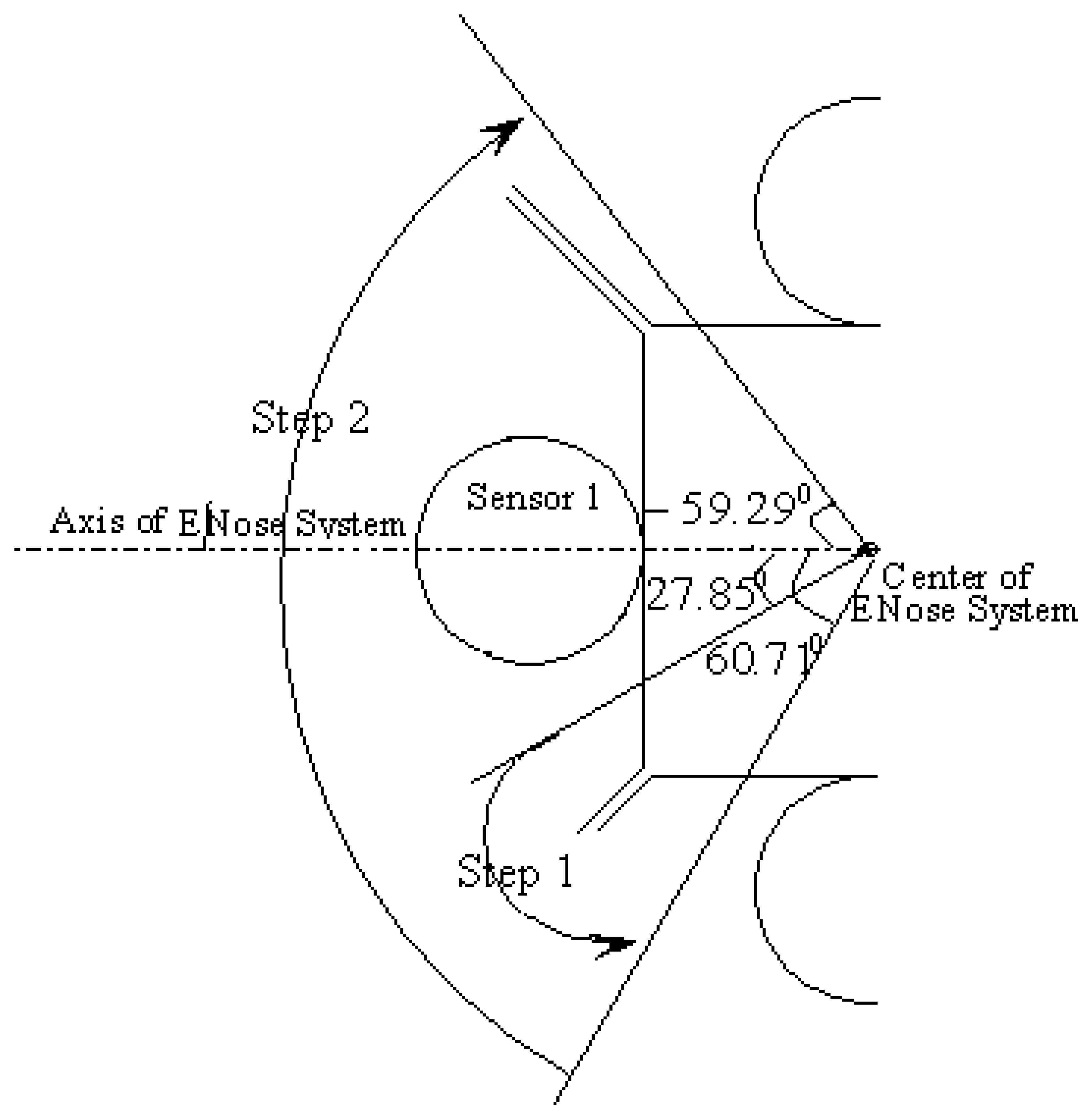
4. Method for dynamic source detection
- a)
- Use the static algorithm to calculate θ1 for source before movement;
- b)
- Repeat step a) when responses of sensors are stable.
- c)
- Generate θi.
5. Simulation and results
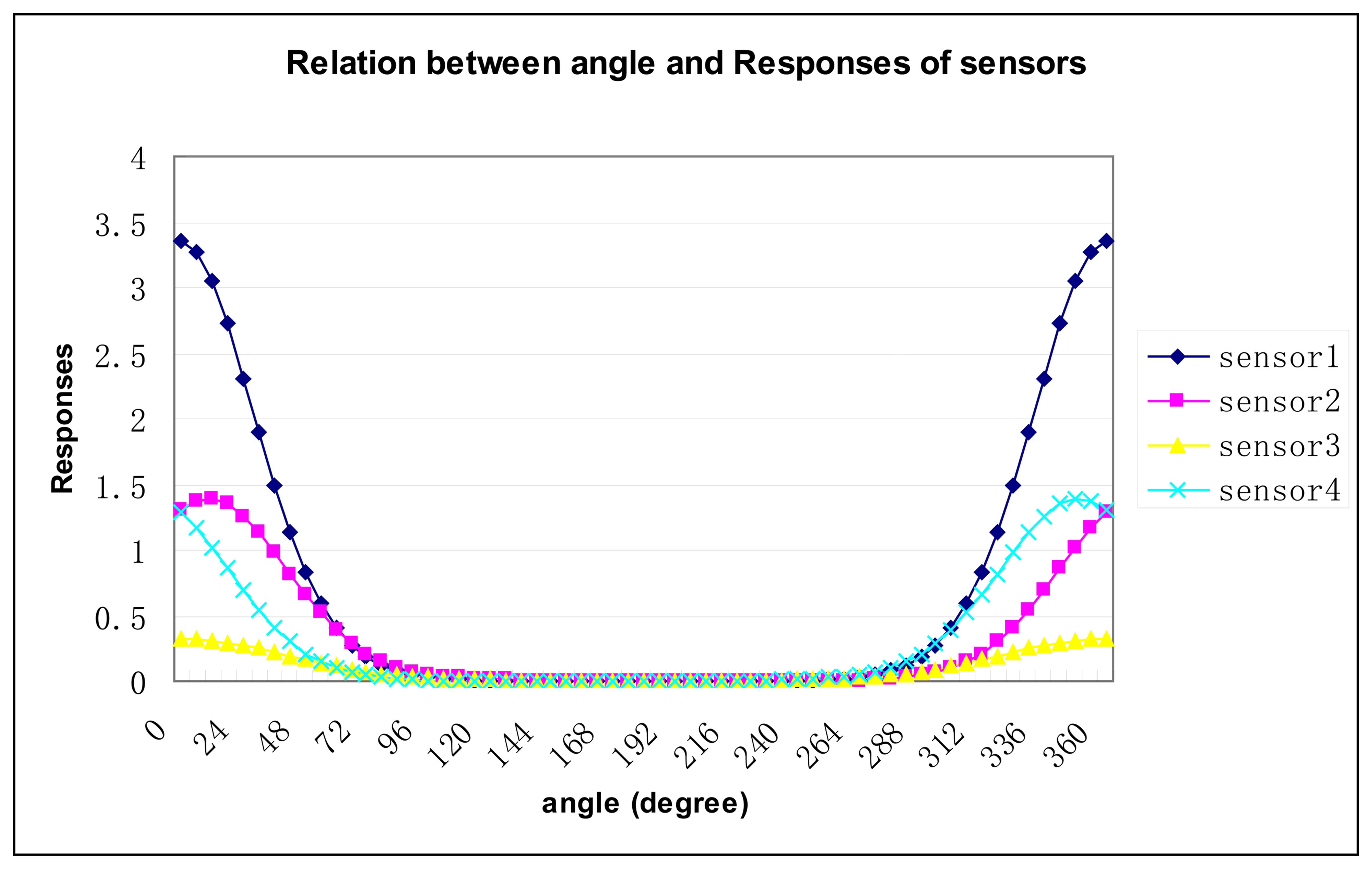
5.1. Static source case
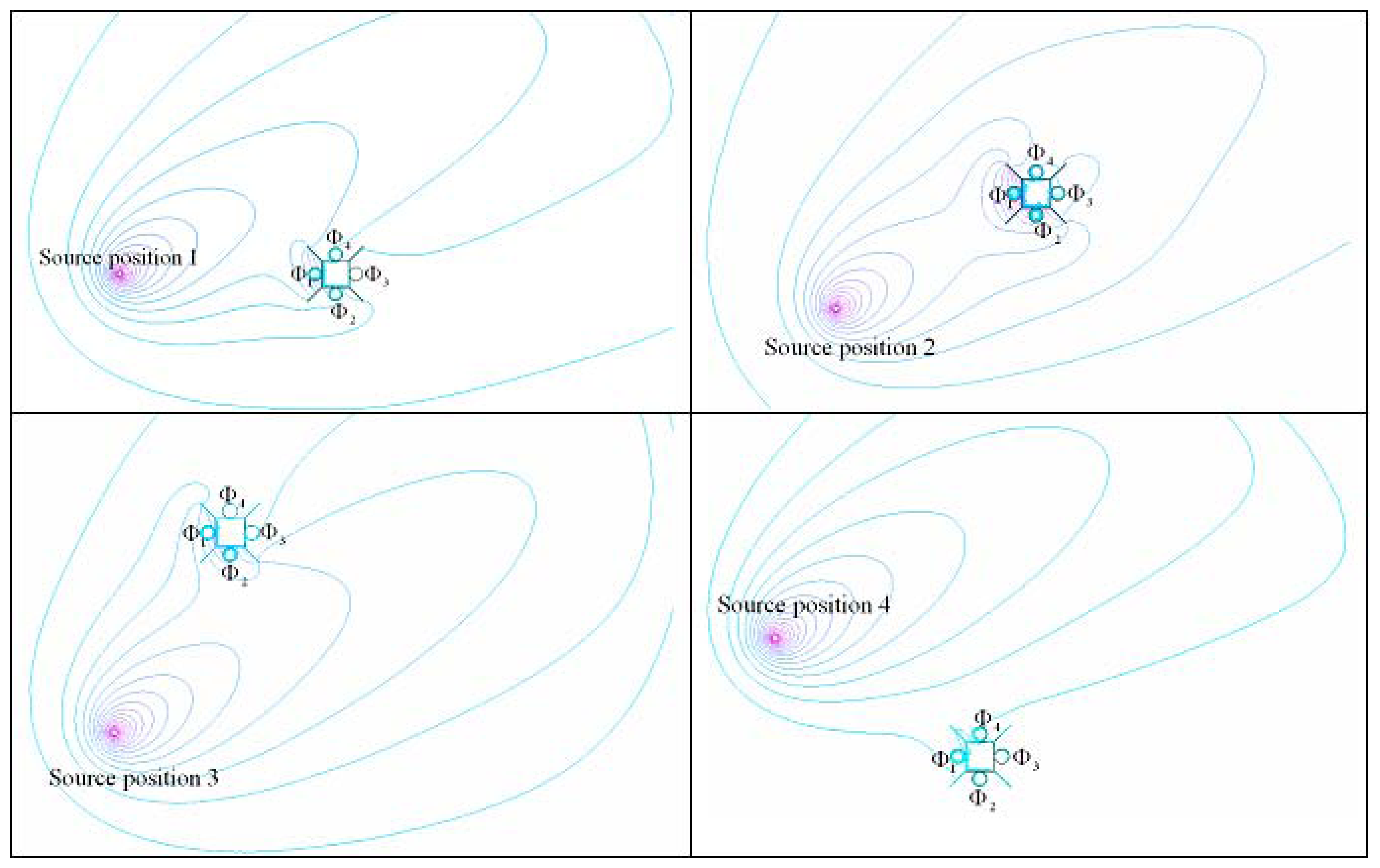
5.2. Dynamic source cases
6. Conclusion and discussion
References and Notes
- Acevedo, F. J.; Maldonado, S.; Dominguez, E.; Narvaez, A.; Lopez, F. Probabilistic support vector machines for multi-class alcohol identification. Sensors and Actuators B: Chemical. In Press, Corrected Proof.
- Yu, H.; Wang, J. Discrimination of LongJing green-tea grade by electronic nose. Sensors and Actuators B: Chemical. In Press, Corrected Proof.
- Bell, G. A.; Watson, A. J. Tastes & Aromas, the chemical senses in science and industry.; University of New South Wales Press: Sydney, 1999. [Google Scholar]
- Peng, Y.; Min, P.; Yuquan, C.; Guang, L. The recognition of Chinese spirits using electronic nose with dynamic method. Engineering in Medicine and Biology Society. Proceedings of the 23rd Annual International Conference of the IEEE, 2001; 2001; pp. 3118–3120. [Google Scholar]
- Brudzewski, K.; Osowski, S.; Markiewicz, T.; Ulaczyk, J. Classification of gasoline with supplement of bio-products by means of an electronic nose and SVM neural network. Sensors and Actuators B: Chemical 2006, 113(1), 135–141. [Google Scholar]
- Sobanski, T.; Szczurek, A.; Nitsch, K.; Licznerski, B. W.; Radwan, W. Electronic nose applied to automotive fuel qualification. Sensors and Actuators B: Chemical 2006, 116(1-2), 207–212. [Google Scholar]
- Scorsone, E.; Pisanelli, A. M.; Persaud, K. C. Development of an electronic nose for fire detection. Sensors and Actuators B: Chemical 2006, 116(1-2), 55–61. [Google Scholar]
- Ampuero, S.; Bosset, J. O. The electronic nose applied to dairy products: a review. Sensors and Actuators B: Chemical 2003, 94(1), 1–12. [Google Scholar]
- Carmel, L. Electronic nose signal restoration--beyond the dynamic range limit. Sensors and Actuators B: Chemical 2005, 106(1), 95–100. [Google Scholar]
- Carmel, L.; Sever, N.; Lancet, D.; Harel, D. An ENose algorithm for identifying chemicals and determining their concentration. Sensors and Actuators B: Chemical 2003, 93(1-3), 77–83. [Google Scholar]
- Haddad, R.; Carmel, L.; Harel, D. A feature extraction algorithm for multi-peak signals in electronic noses. Sensors and Actuators B: Chemical. In Press, Corrected Proof.
- Carmel, L.; Levy, S.; Lancet, D.; Harel, D. A feature extraction method for chemical sensors in electronic noses. Sensors and Actuators B: Chemical 2003, 93(1-3), 67–76. [Google Scholar]
- Padilla, M.; Montoliu, I.; Pardo, A.; Perera, A.; Marco, S. Feature extraction on three way ENose signals. Sensors and Actuators B: Chemical 2006, 116(1-2), 145–150. [Google Scholar]
- Hong, C.; Goubran, R. A.; Mussivand, T. Improving the classification accuracy in electronic noses using multi-dimensional combining (MDC). Sensors, Proceedings of IEEE, 2004; 2004; pp. 587–590. [Google Scholar]
- Qin, S. J.; Wu, Z. J. A new approach to analyzing gas mixtures. Sensors and Actuators B: Chemical 2001, 80(2), 85–88. [Google Scholar]
- Loutfi, A.; Coradeschi, S. Relying on an electronic nose for odor localization. Virtual and Intelligent Measurement Systems. VIMS '02. 2002 IEEE International Symposium on, 2002; 2002; pp. 46–50. [Google Scholar]
- Marques, L.; De Almeida, A. T. Electronic nose-based odour source localization. Advanced Motion Control. Proceedings. 6th International Workshop on, 2000; 2000; pp. 36–40. [Google Scholar]
- Jatmiko, W.; Ikemoto, Y.; Matsuno, T.; Fukuda, T.; Sekiyama, K. Distributed odor source localization in dynamic environment. Sensors, IEEE, 2005; 2005; p. p 4 pp. [Google Scholar]
- Matthes, J.; Groll, L.; Keller, H. B. Source localization by spatially distributed electronic noses for advection and diffusion. Signal Processing, IEEE Transactions on [see also Acoustics, Speech, and Signal Processing, IEEE Transactions on] 2005, 53(5), 1711–1719. [Google Scholar]
- http://www.figarosensor.com/gaslist.html, September, 28th 2006
- http://www.mathworks.com/access/helpdesk_r13/help/toolbox/curvefit/ch_fitt9.html, October, 31st 2006


| Real direction | 60° | 120° | 180° | −120° | −60° | 360°(0°) | Mean error | |
|---|---|---|---|---|---|---|---|---|
| Advection case | C1(×102) | 0.4082 | 0.0054 | 0.0005 | 0.0054 | 0.4082 | 3.355 | ------ |
| C2(×102) | 0.3938 | 0.0132 | 0.0012 | 0.0023 | 0.0995 | 1.291 | ------ | |
| C4(×102) | 0.0995 | 0.0023 | 0.0012 | 0.0132 | 0.3938 | 1.297 | ------ | |
| C2/C1 | 0.9647 | 2.444 | 2.400 | 0.4259 | 0.2438 | 0.3848 | ------ | |
| C4/C1 | 0.2438 | 0.4259 | 2.400 | 2.444 | 0.9647 | 0.3866 | ------ | |
| Measured source direction(θ) | 60.71° | 120.54° | 177.41° | −119.46° | −59.29° | 360°(0°) | ------ | |
| Relative error | 1.17% | 0.45% | 1.46% | 0.45% | 1.17% | 0.00% | 0.78% | |
| Crosswind case | C1(×102) | 1.570 | 0.0208 | 0.0003 | 0.0005 | 0.0456 | 2.236 | ------ |
| C2(×102) | 1.765 | 0.0573 | 0.0009 | 0.0002 | 0.0092 | 0.9000 | ------ | |
| C4(×102) | 0.3172 | 0.0072 | 0.0007 | 0.0014 | 0.0513 | 0.7801 | ------ | |
| C2/C1 | 1.124 | 2.755 | 3.000 | 0.4000 | 0.2018 | 0.4025 | ------ | |
| C4/C1 | 0.2020 | 0.3462 | 2.333 | 2.800 | 1.125 | 0.3489 | ------ | |
| Measured source direction(θ) | 61.46° | 116.38° | 175.01° | −116.68° | −62.81° | 360.11° | ------ | |
| Relative error | 2.38% | 3.11% | 2.85% | 2.85% | 4.47% | 0.03% | 2.62% | |
| P | T (s) | C1 (×102ppm) | C2 (×102ppm) | C4 (×102ppm) | C2 / C1 | C4 / C1 | Source direction(θ) | Relative error | |
|---|---|---|---|---|---|---|---|---|---|
| measured | real | ||||||||
| - | 0 | 0 | 0 | 0 | - | - | - | - | - |
| 1 | 20 | 1.893 | 1.128 | 0.5367 | 0.5959 | 0.2835 | 27.85° | 30° | 7.72% |
| 2 | 21 | 1.6755 | 1.007 | 0.4514 | 0.6010 | 0.2694 | 28.37° | 45° | 58.62% |
| 36.14° | 19.69% | ||||||||
| 3 | 31 | 0.4082 | 0.3938 | 0.0995 | 0.9647 | 0.2438 | 60.71° | 60° | 1.17% |
| 4 | 33 | 0.8548 | 0.5971 | 0.1210 | 0.6985 | 0.1416 | 38.07° | 0° | 100.00% |
| null | -- | ||||||||
| 5 | 73 | 0.4082 | 0.0995 | 0.3938 | 0.2438 | 0.9647 | −59.29° | −60° | 1.17% |
© 2006 by MDPI ( http://www.mdpi.org). Reproduction is permitted for noncommercial purposes.
Share and Cite
Cai, J.; Levy, D.C. Tracking Dynamic Source Direction with a Novel Stationary Electronic Nose System. Sensors 2006, 6, 1537-1554. https://doi.org/10.3390/s6111537
Cai J, Levy DC. Tracking Dynamic Source Direction with a Novel Stationary Electronic Nose System. Sensors. 2006; 6(11):1537-1554. https://doi.org/10.3390/s6111537
Chicago/Turabian StyleCai, Jie, and David C. Levy. 2006. "Tracking Dynamic Source Direction with a Novel Stationary Electronic Nose System" Sensors 6, no. 11: 1537-1554. https://doi.org/10.3390/s6111537
APA StyleCai, J., & Levy, D. C. (2006). Tracking Dynamic Source Direction with a Novel Stationary Electronic Nose System. Sensors, 6(11), 1537-1554. https://doi.org/10.3390/s6111537