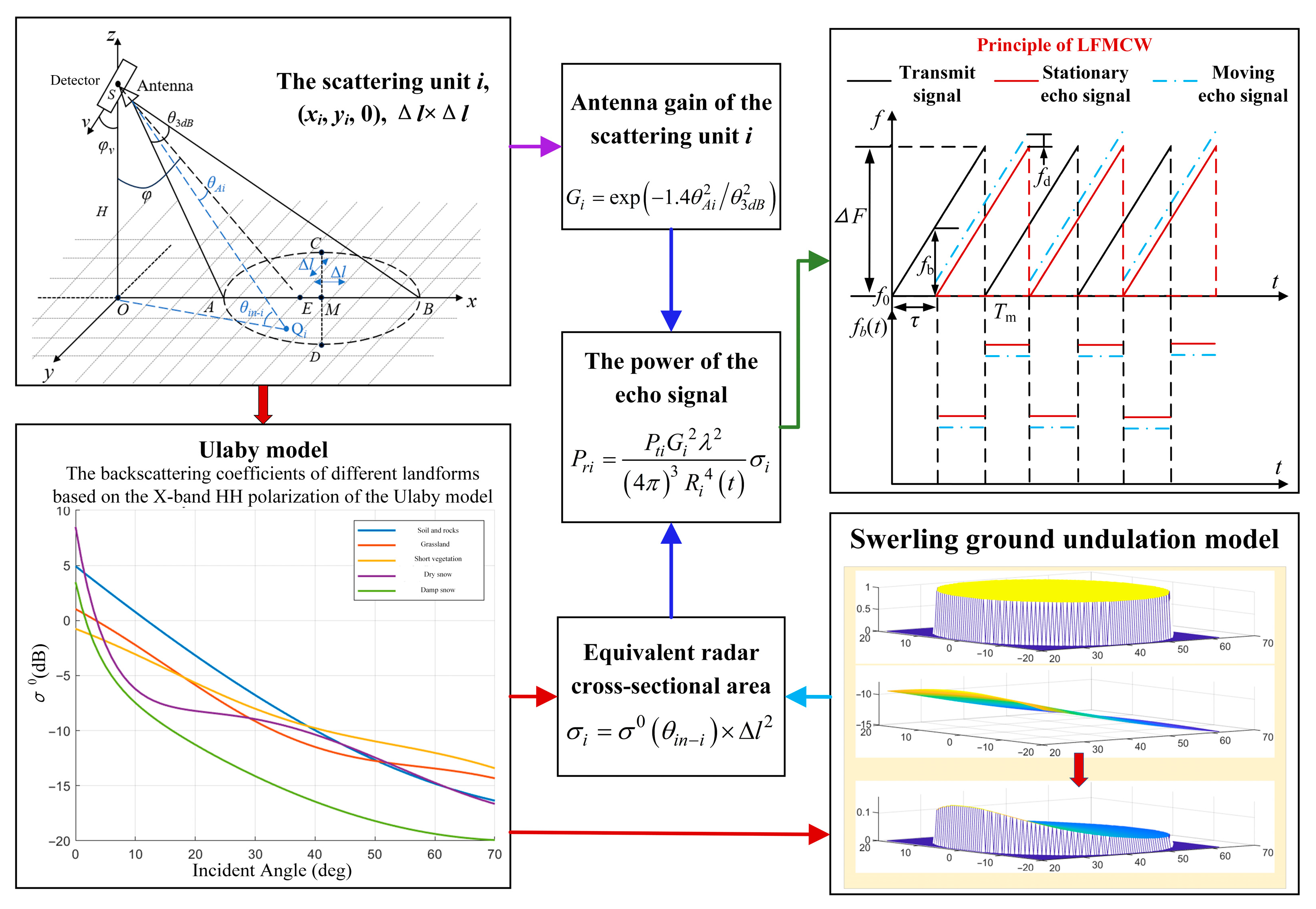
Figure 1.
Establishment of multi-terrain echo model.
Figure 1.
Establishment of multi-terrain echo model.
Figure 2.
Time domain signals of target echo with single jamming: (a) NAM, (b) NFM, (c) SAM, (d) SFM, (e) RFT, and (f) VFT.
Figure 2.
Time domain signals of target echo with single jamming: (a) NAM, (b) NFM, (c) SAM, (d) SFM, (e) RFT, and (f) VFT.
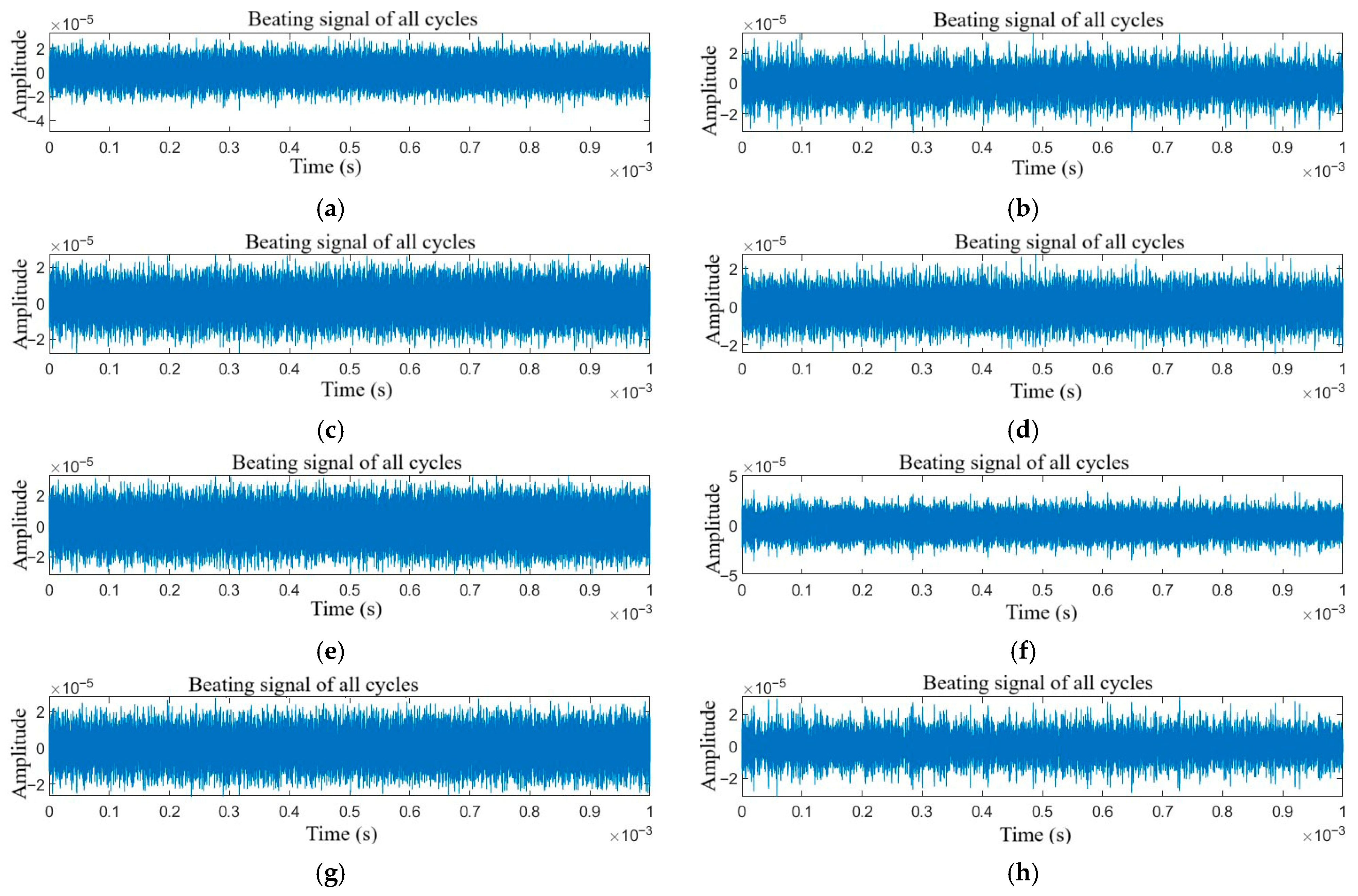
Figure 3.
Time domain signals of target echo with compound jamming: (a) NAM + RFT, (b) NAM + VFT, (c) NFM + RFT, (d) NFM + VFT, (e) SAM + RFT, (f) SAM + VFT, (g) SFM + RFT, and (h) SFM + VFT.
Figure 3.
Time domain signals of target echo with compound jamming: (a) NAM + RFT, (b) NAM + VFT, (c) NFM + RFT, (d) NFM + VFT, (e) SAM + RFT, (f) SAM + VFT, (g) SFM + RFT, and (h) SFM + VFT.
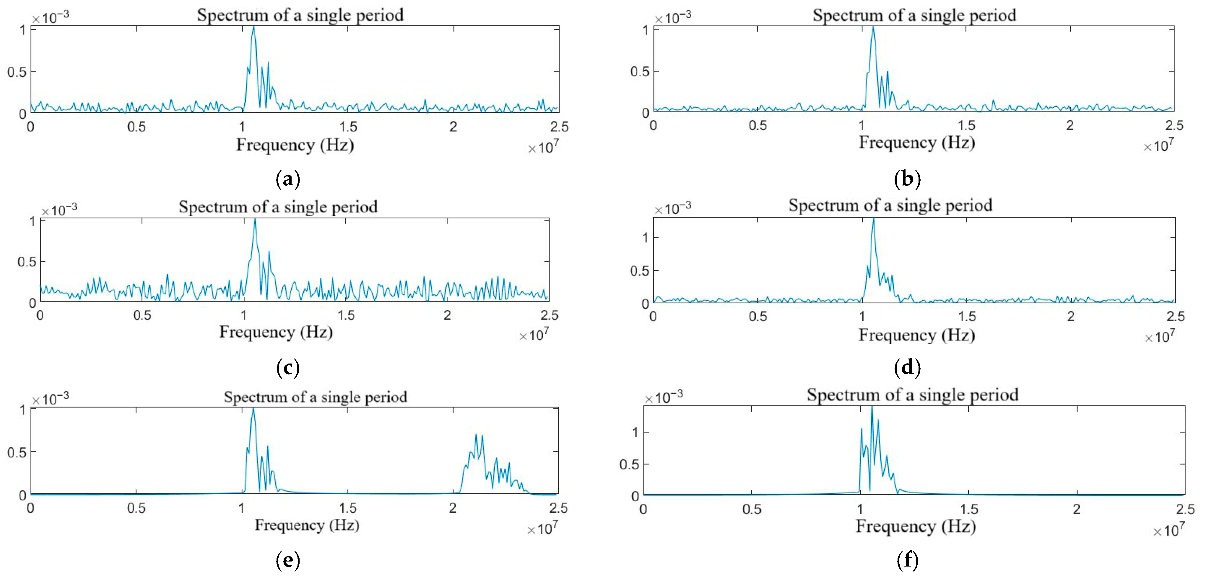
Figure 4.
Spectrum diagram of the target echo with single jamming: (a) NAM, (b) NFM, (c) SAM, (d) SFM, (e) RFT, and (f) VFT.
Figure 4.
Spectrum diagram of the target echo with single jamming: (a) NAM, (b) NFM, (c) SAM, (d) SFM, (e) RFT, and (f) VFT.
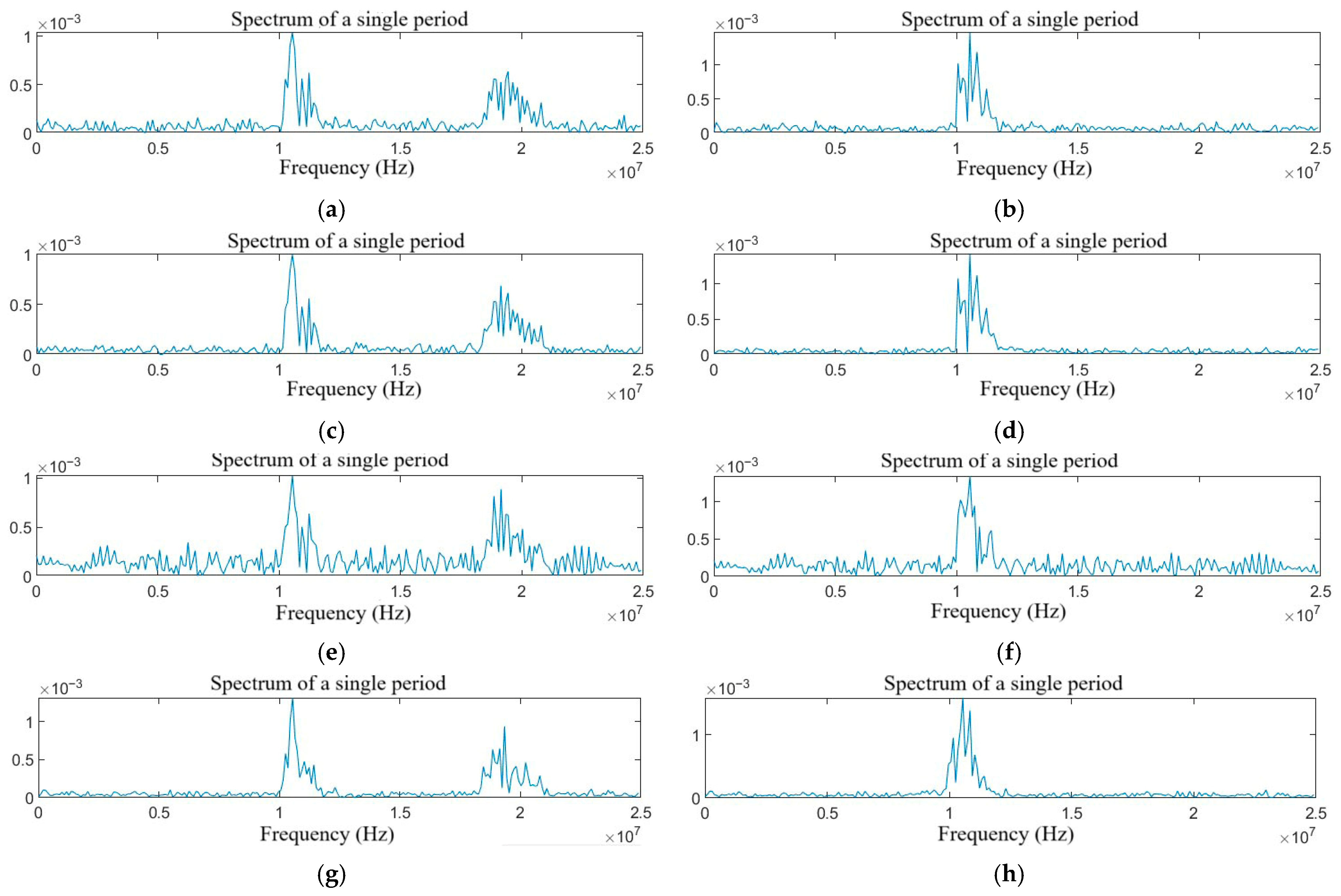
Figure 5.
Spectrum diagram of the target echo with compound jamming: (a) NAM + RFT, (b) NAM + VFT, (c) NFM + RFT, (d) NFM + VFT, (e) SAM + RFT, (f) SAM + VFT, (g) SFM + RFT, and (h) SFM + VFT.
Figure 5.
Spectrum diagram of the target echo with compound jamming: (a) NAM + RFT, (b) NAM + VFT, (c) NFM + RFT, (d) NFM + VFT, (e) SAM + RFT, (f) SAM + VFT, (g) SFM + RFT, and (h) SFM + VFT.
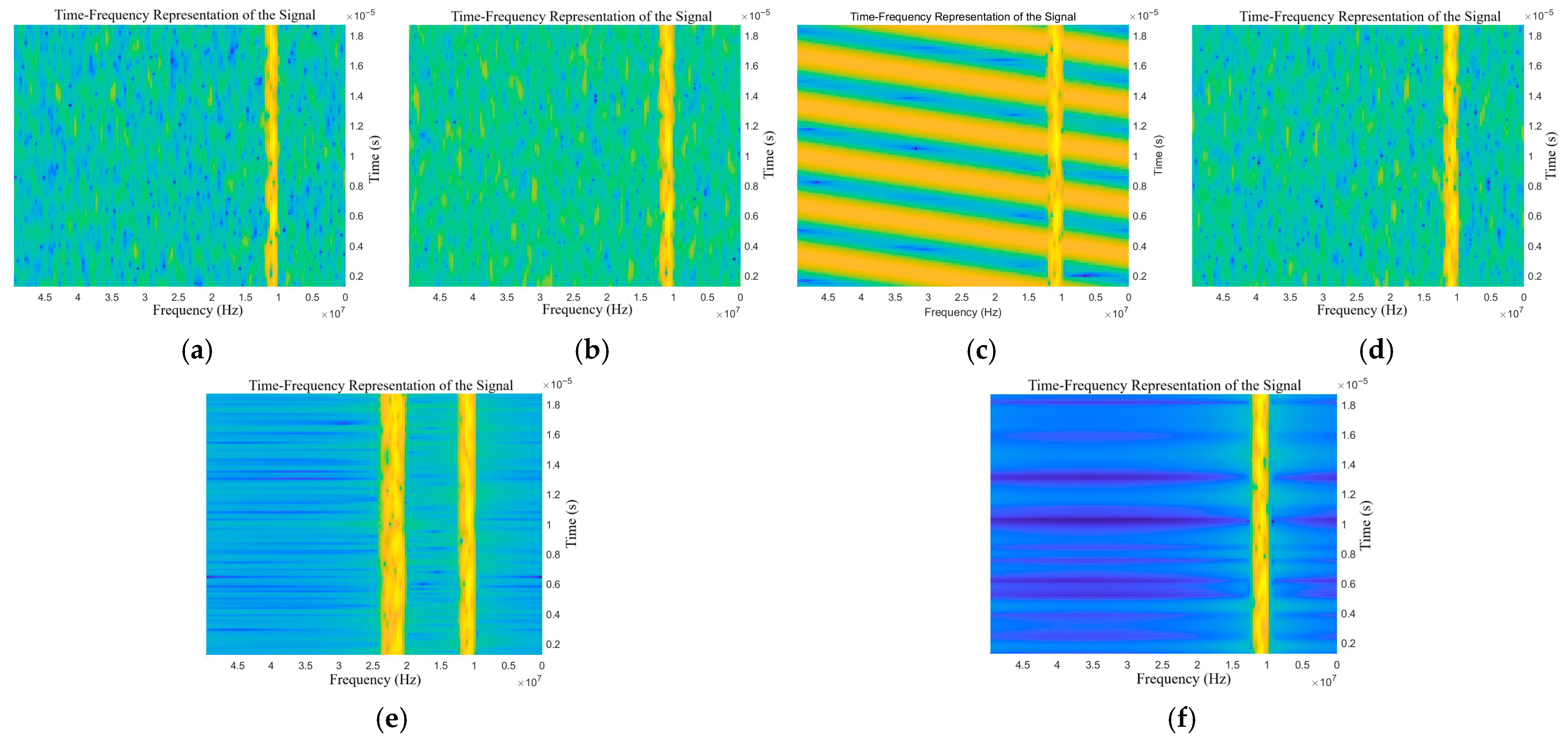
Figure 6.
Time-frequency representations of the target echo with single jamming: (a) NAM, (b) NFM, (c) SAM, (d) SFM, (e) RFT, and (f) VFT.
Figure 6.
Time-frequency representations of the target echo with single jamming: (a) NAM, (b) NFM, (c) SAM, (d) SFM, (e) RFT, and (f) VFT.
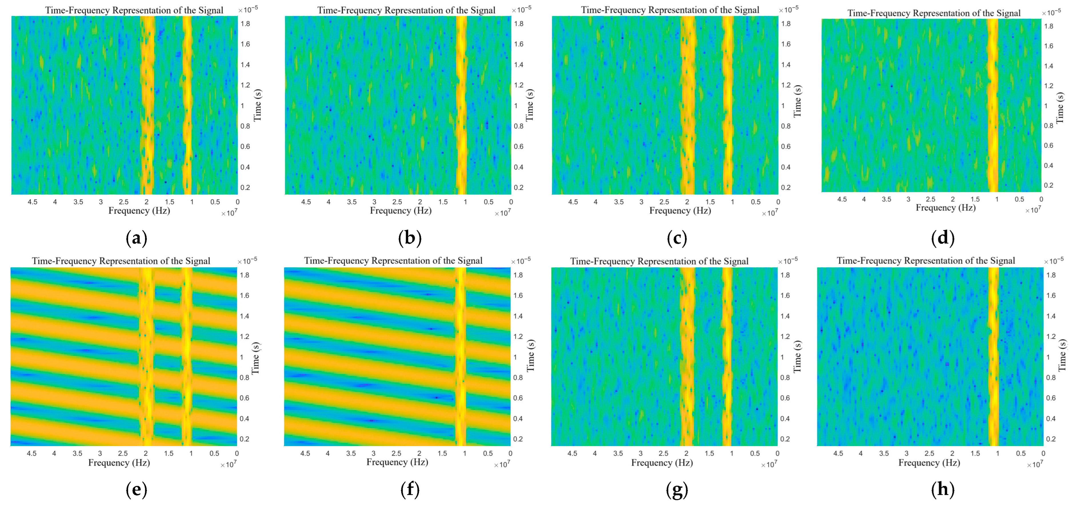
Figure 7.
Time-frequency representations of the target echo with compound jamming: (a) NAM + RFT, (b) NAM + VFT, (c) NFM + RFT, (d) NFM + VFT, (e) SAM + RFT, (f) SAM + VFT, (g) SFM + RFT, and (h) SFM + VFT.
Figure 7.
Time-frequency representations of the target echo with compound jamming: (a) NAM + RFT, (b) NAM + VFT, (c) NFM + RFT, (d) NFM + VFT, (e) SAM + RFT, (f) SAM + VFT, (g) SFM + RFT, and (h) SFM + VFT.
Figure 8.
Determination of jamming recognition information.
Figure 8.
Determination of jamming recognition information.
Figure 9.
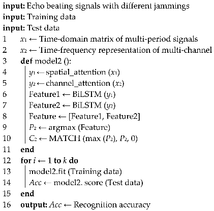
Schematic diagram of the TFWF-AM jamming recognition model.
Figure 9.
Schematic diagram of the TFWF-AM jamming recognition model.
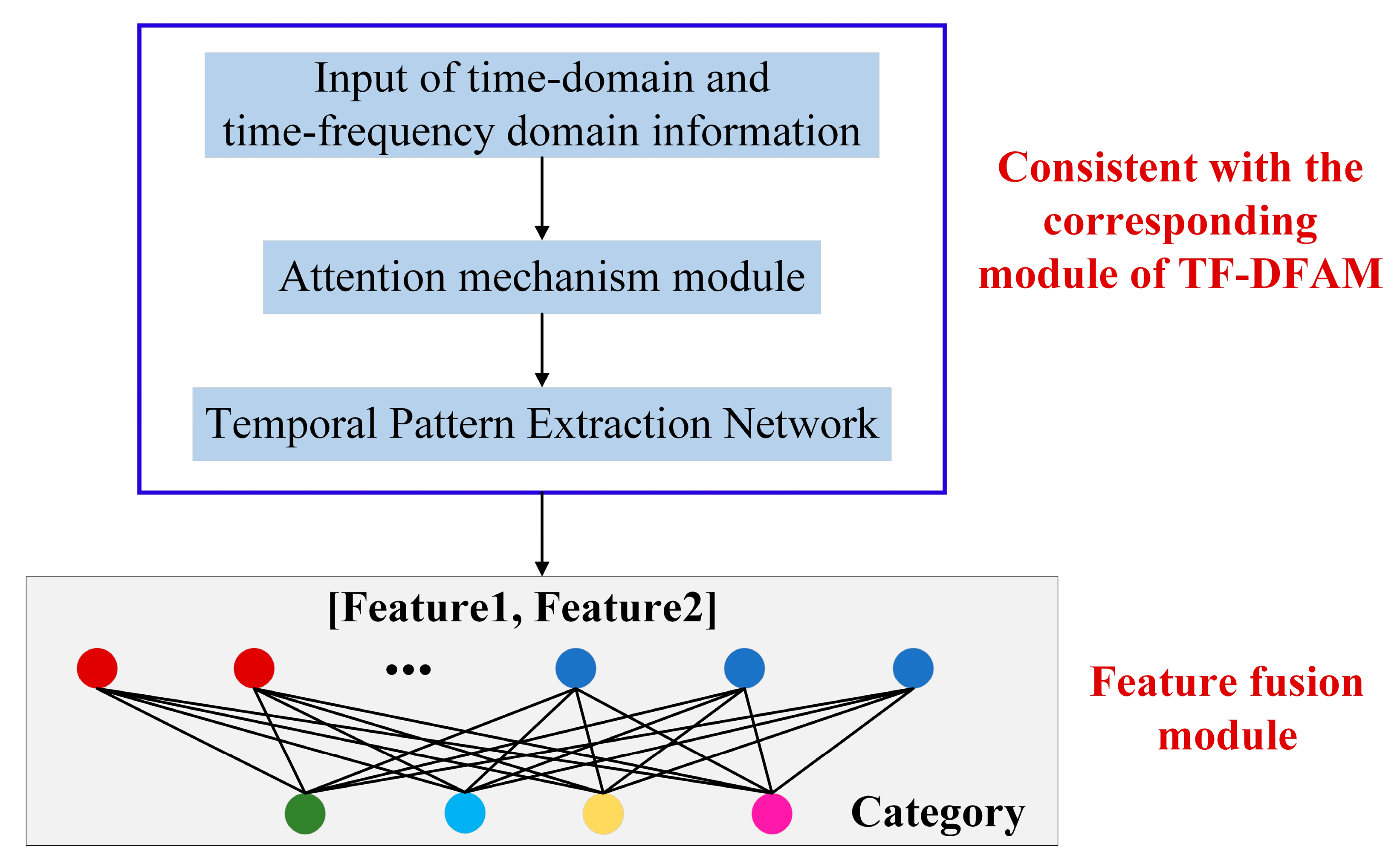
Figure 10.
Schematic diagram of the TFFF-AM jamming recognition model.
Figure 10.
Schematic diagram of the TFFF-AM jamming recognition model.
Figure 11.
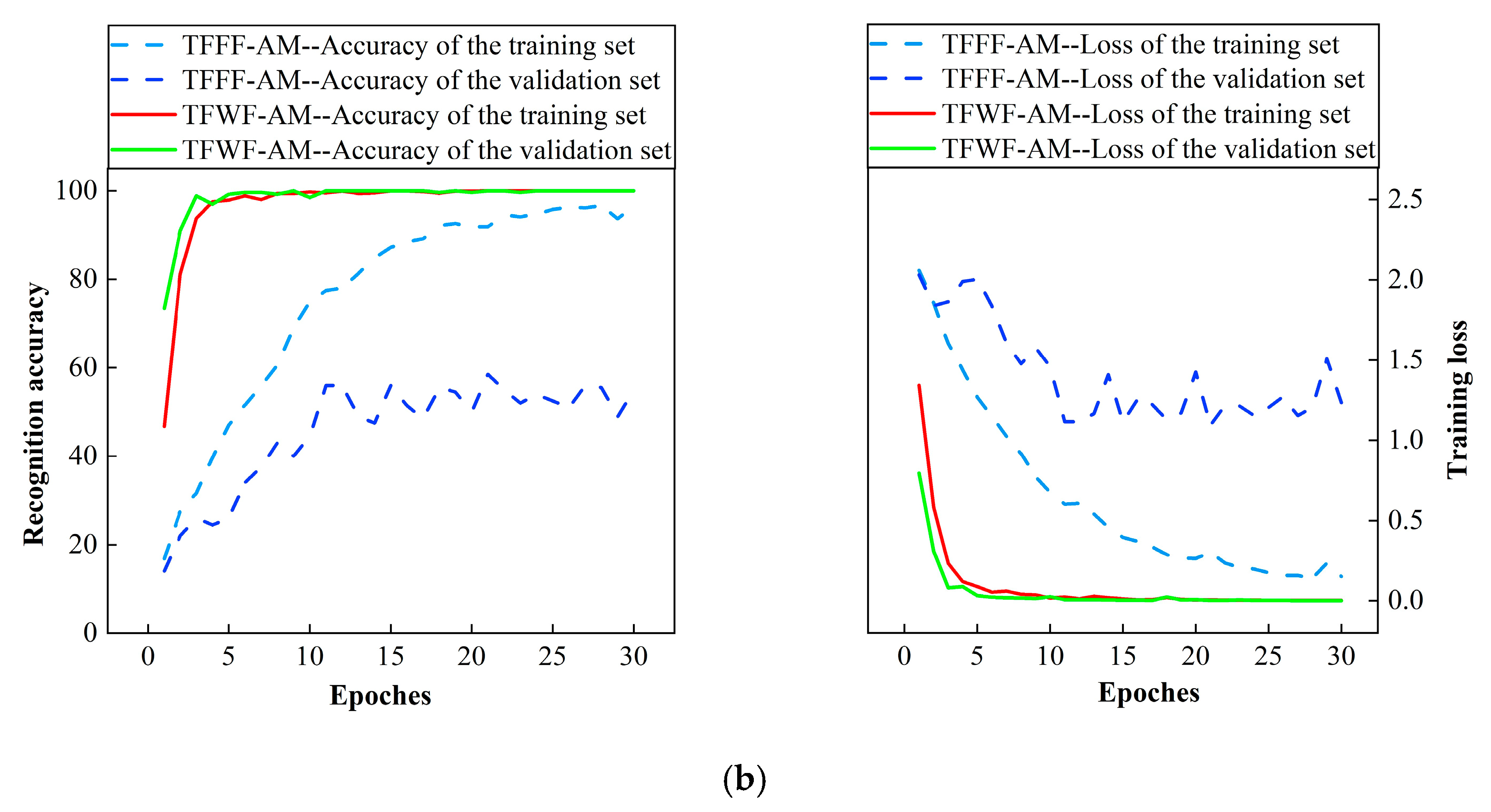
Accuracy graph of training process: (a) the recognition accuracy and loss rate of the two models for single jamming and (b) the recognition accuracy and loss rate of the two models for compound jamming.
Figure 11.
Accuracy graph of training process: (a) the recognition accuracy and loss rate of the two models for single jamming and (b) the recognition accuracy and loss rate of the two models for compound jamming.
Figure 12.
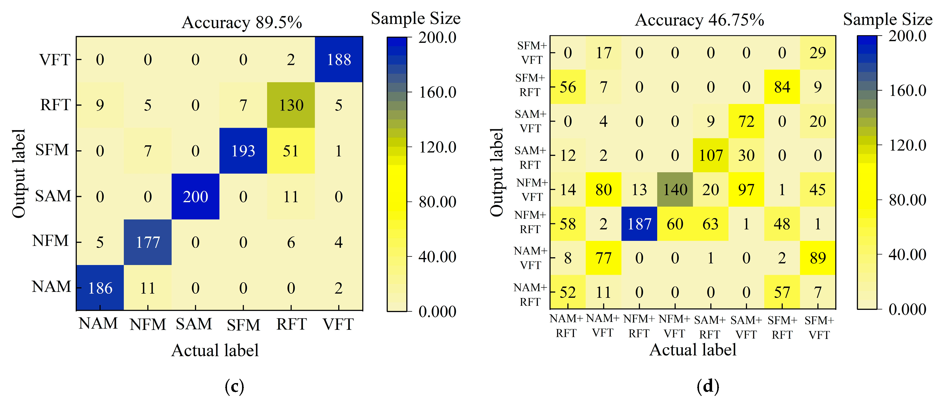
The recognition results of the time-frequency fusion attention mechanism for different jamming: (a) the recognition results of the TFWF-AM model for single jamming, (b) the recognition results of the TFWF-AM model for compound jamming, (c) the recognition results of the TFFF-AM model for single jamming, and (d) the recognition results of the TFFF-AM model for compound jamming.
Figure 13.
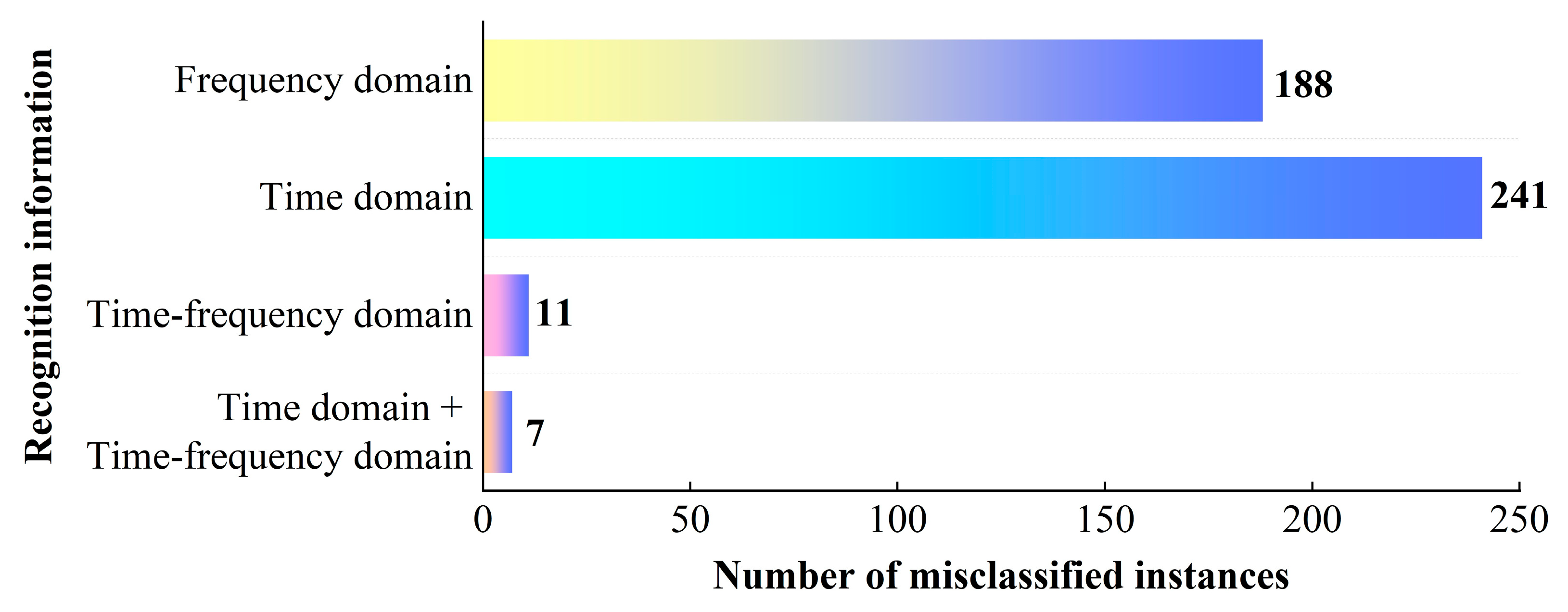
The number of misclassified instances under different jamming recognition information.
Figure 13.
The number of misclassified instances under different jamming recognition information.
Figure 14.
Comparison of this model with existing algorithm models for the compound jamming sample set.
Figure 14.
Comparison of this model with existing algorithm models for the compound jamming sample set.
Table 1.
Expressions of different types of jamming.
Table 1.
Expressions of different types of jamming.
| Expressions |
|---|
Blanket
jamming | NAM | |
| NFM | |
| SAM | |
| SFM | |
Deceptive
jamming | RFT | |
| VFT | |
Table 2.
Main parameters of target echo model.
Table 2.
Main parameters of target echo model.
| Parameters | Definition | Values |
|---|
| f0 | Carrier frequency | 8 GHz |
| Tm | Modulation period | 4 × 10⁻⁵ s |
| v | Velocity | 500 m/s |
| c | Light velocity | 3 × 10⁸ m/s |
| ΔF | Frequency modulation deviation | 300 MHz |
| R0 | The initial distance from target to detector | 100 m |
| Pt | Transmission power | 1 W |
| Fs | The sampling frequency of beating signal | 50 MHz |
Table 3.
Fitting parameters of the multi-terrain Ulaby model.
Table 3.
Fitting parameters of the multi-terrain Ulaby model.
| Terrains | Incidence Angle (θ) | Fitting Value |
|---|
| P1 | P2 | P3 | P4 | P5 | P6 |
|---|
| Grassland | 0 | 80 | −33.288 | 32.980 | 0.510 | −1.343 | 4.874 | −3.142 |
| Dry snow | 0 | 75 | −13.298 | 20.048 | 10.0 | 4.529 | 2.927 | −1.173 |
| Soil and rock surface | 0 | 80 | 4.337 | 6.666 | −0.107 | −29.709 | 0.863 | −1.365 |
| Short vegetation | 0 | 80 | −99.0 | 97.417 | 0.114 | −0.837 | 5.0 | −2.984 |
| Wet snow | 0 | 80 | 10.020 | 7.909 | 15.0 | 30.0 | 0.828 | 2.073 |
Table 4.
Jamming recognition sample sets and quantity statistics.
Table 4.
Jamming recognition sample sets and quantity statistics.
| Type of Jamming | The Quantity of Samples |
|---|
| Single jamming | NAM | 200 |
| NFM | 200 |
| SAM | 200 |
| SFM | 200 |
| RFT | 200 |
| VFT | 200 |
| Compound jamming | NAM + RFT | 200 |
| NAM + VFT | 200 |
| NFM + RFT | 200 |
| NFM + VFT | 200 |
| SAM + RFT | 200 |
| SAM + VFT | 200 |
| SFM + RFT | 200 |
| SFM + VFT | 200 |
Table 5.
Performance comparison of TFWF-AM and TFFF-AM jamming recognition models.
Table 5.
Performance comparison of TFWF-AM and TFFF-AM jamming recognition models.
| Types of Jamming | Single Jamming | Compound Jamming |
|---|
| Recognition model | TFFF-AM | TFWF-AM | Parameter comparison | TFFF-AM | TFWF-AM | Parameter comparison |
| Number of misclassified instances | 126 | 1 | −125 | 852 | 7 | −845 |
| NAPT | 1 | 0.524 | −47.6% | 1 | 0.464 | −53.6% |
| Recognition accuracy | 89.50% | 99.92% | +10.42% | 46.75% | 99.56% | +52.81% |
Table 6.
Analysis of model embeddability.
Table 6.
Analysis of model embeddability.
| Parameters | TFWF-AM | MLCJRN [37] | MANet [38] | JRNet [39] |
|---|
| FLOPs (M) | 100.83 | 108.5 | 190.0 | 1820.0 |
| Parameters (M) | 2.48 | 0.98 | 2.54 | 11.69 |
| Memory requirements (M) | 2.94 | - | - | - |
Table 7.
The recognition effect of TFWF-AM for single jamming.
Table 7.
The recognition effect of TFWF-AM for single jamming.
| Types of Jamming | NAM | NFM | SAM | SFM | RFT | VFT |
|---|
| Precision | 100% | 99.5% | 100% | 100% | 100% | 100% |
| Recall | 100% | 100% | 100% | 99.5% | 100% | 100% |
| F1 score | 1.0 | 0.997 | 1.0 | 0.997 | 1.0 | 1.0 |
| Accuracy | 99.92% |
Table 8.
The recognition effect of TFWF-AM for compound jamming.
Table 8.
The recognition effect of TFWF-AM for compound jamming.
| Types of Jamming | NAM + RFT | NAM + VFT | NFM + RFT | NFM + VFT | SAM + RFT | SAM + VFT | SFM + RFT | SFM + VFT |
|---|
| Precision | 99.5% | 100% | 98.03% | 99% | 100% | 100% | 100% | 100% |
| Recall | 100% | 97.5% | 99.5% | 99.5% | 100% | 100% | 100% | 100% |
| F1 score | 0.997 | 0.987 | 0.988 | 0.992 | 1.0 | 1.0 | 1.0 | 1.0 |
| Accuracy | 99.56% |
Table 9.
The misclassification quantity of different jamming recognition information.
Table 9.
The misclassification quantity of different jamming recognition information.
Recognition
Information | Time Domain +
Time-Frequency Domain | Time-Frequency Domain | Time
Domain | Frequency
Domain |
|---|
| Misclassification quantity | 7 | 11 | 241 | 188 |
Table 10.
The recognition results of the TFWF-AM model for the new type of jamming.
Table 10.
The recognition results of the TFWF-AM model for the new type of jamming.
| Types of Jamming | CI | ISR | SMSP |
|---|
| Sample size | 200 | 200 | 200 |
| The number of correctly classified samples | 200 | 200 | 200 |
| Recognition accuracy | 100% |
Table 11.
The recognition results of the model for compound jamming under different SNR.
Table 11.
The recognition results of the model for compound jamming under different SNR.
| SNR | −5 | −3 | 0 | 3 | 5 |
|---|
| Recognition accuracy | 46.8% | 69.4% | 82.4% | 80.2% | 84.6% |
Table 12.
The comparison of recognition accuracy between this model and the existing algorithm.
Table 12.
The comparison of recognition accuracy between this model and the existing algorithm.
| Deep Learning Algorithm | Recognition Accuracy | Machine Learning Algorithm | Recognition Accuracy |
|---|
| TFFF-AM | 46.75% | XGBoost | 65.25% |
| TFWF-AM | 99.56% | Logistic regression | 79.63% |
| ResNet | 96.3% | Decision tree | 49.5% |
| AlexNet | 12.4% | AdaBoost | 36.88% |

